Vertical distribution of Galactic disk stars:

High resolution spectra data of red clump stars towards the NGP have been obtained with the high resolution spectrograph Elodie at OHP for Tycho-2 selected stars. Combined with Hipparcos local analogues, we determine both the gravitational force law perpendicular to the Galactic plane, and the total surface mass density and thickness of the Galactic disk. The surface mass density of the Galactic disk within 800 pc derived from this analysis is $\Sigma$ ($|z|<$800   $\rm{pc})$ = 76   $\mathrm{M}_{\odot}\mathrm{pc}^{-2}$ and, removing the dark halo contribution, the total disk mass density is $\Sigma_{0}$ = 67  $\mathrm{M}_{\odot}\mathrm{pc}^{-2}$ at solar radius. The thickness of the total disk mass distribution is dynamically measured for the first time and is found to be 390${}^{+330}_{-120}$ pc in relative agreement with the old stellar disk scaleheight. All dynamical evidences concerning the structure of the disk (its local volume density –i.e. the Oort limit–, its surface density and its thickness) are compatible with our current knowledge of the corresponding stellar disk properties.

1 Introduction

We present a new dynamical determination of the Galactic potential and $K_{z}$ force perpendicular to the Galactic plane. We measure the surface mass density of the Galactic disk (i.e. the total amount of disk mass in a column perpendicular to the Galactic plane) and also the thickness of the vertical mass distribution of the disk at the Sun. They are fundamental parameters of the Galaxy, determining the disk contribution to the Galactic potential and to the rotation curve. They also give valuable constraints to the disk properties. The “$K_{z}$ problem” is traditional in Galactic dynamics and subsequent derivation of the total mass density $\rho_{0}$ (the Oort limit) has a long history begining with Kapteyn (1922) and Oort (1932). Comprehensive review may be found in Kerr & Lynden-Bell (1986) and in Kuijken (1995). Most recent works may be found in Crézé et al. (1998a) and in Holmberg & Flynn (2000) and references within. They favor a low Oort limit $\rho$(z=0) = 0.076–0.10 $\mathrm{M}_{\odot}\mathrm{pc}^{-3}$. Previous surface mass density determinations (including only disk contribution and removing the local halo contribution) are $\Sigma_{0}$= 52$\pm 13\,\mathrm{M}_{\odot}\mathrm{pc}^{-2}$ (Flynn & Fuchs 1994), $\Sigma_{0}$ = 48$\pm 9\,\mathrm{M}_{\odot}\mathrm{pc}^{-2}$, (Kuijken and Gilmore 1991).

Here, to investigate the vertical structure and potential of the Galactic disk, we have observed a sample of red clump giants towards the North Galactic Pole with a high resolution spectrograph (Elodie at OHP). Observations and properties of the sample are given in the paper I of this series (Soubiran et al 2002) where we detail the measurements of abundances, absolute magnitudes and radial velocities, and describe the sample properties. Atmospheric parameters and absolute magnitudes of stars have been obtained with the TGMET method (Katz et al. 1998) by comparing the observed spectra to the TGMET library of similar spectra of Hipparcos stars with known characteristics. The method is applied in Paper I (Soubiran et al 2002). The library is built from the ELODIE database described in Prugniel & Soubiran (2001). The main advantage of selecting red clump stars is that their luminosity function is sharply defined in a small magnitude interval minimizing completeness bias (Malmquist or Lutz-Kelker), making more accurate their corrections. This remote sample has been analysed combined to a local sample of similar Hipparcos stars in a sphere of 125 pc around the Sun.

In Sect. 2, we describe the red clump sample definition extracted from the general sample of bright red stars observed at OHP (see Paper I) and the correction for the Lutz-Kelker bias for the associated Hipparcos subsample. The method to determine the potential $\Phi(z)$ and vertical force $K_{z}$ is classical but calls for some algebra because the NGP samples cover wide solid angles on the sky (Sect. 3). Results are presented in Sect. 4: we confirm with this independent stellar sample previous findings concerning the disk surface mass density and we present the first observational constrain on the total thickness of the mass distribution of the Galactic disk.

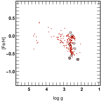
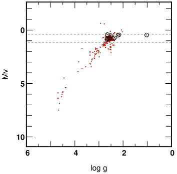
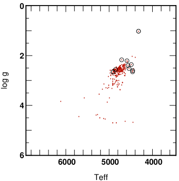
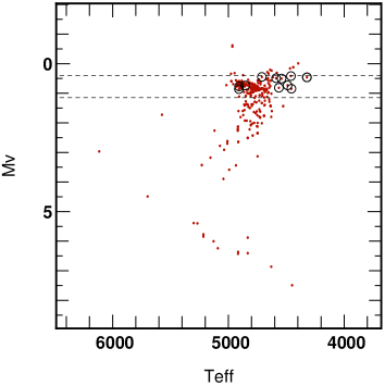
Figure 1: Properties of the observed stars. Horizontal dashed lines indicate our selection procedure for the red giant clump sample. Circles denote stars belonging to our $M_{\rm V}$ selection that are probably not clump stars (see text).

2 The giant clump samples

Our sample consists of stars selected out of the Tycho-2 catalogue (ESA 1997) and is described in Paper I (Soubiran et al 2002). A selection in $B-V$ colour has been applied to increase the number of red clump stars with respect to dwarfs, subgiants, RGB and AGB stars. We have chosen the colour interval 0.9 $<B-V<$ 1.1 that optimizes the detection of red clump stars. The lower $B-V$ limit at 0.9 rejects the brightest main sequence stars ($M_{\textrm{v}}<5$), some subgiants and also most giants of the blue horizontal branch (the ”clump stars” with the lowest metallicities). The upper $B-V$ limit at 1.1 rejects most of RGB and AGB stars.
The selection criteria maximise the number of clump stars with respect to dwarfs and red giants along the ascending branch but remain a mixture of those three types of objects. Our stellar parameters determination (absolute magnitude) allows to separate red clump stars from dwarfs and from other giant stars. We combine our remote sample with a local Hipparcos sample built with the same criteria based on colours and absolute magnitudes. This procedure is sketched in subsection 2.1. The distance limited sample is built, using the Hipparcos catalog. This sample is affected by the Lutz-Kelker bias, its composition as well as the bias correction are given in subsection 2.2.

2.1 The NGP cone samples

In this study we are interested in the bright stellar population defined by the red clump stars allowing to probe stellar populations far from the mid-plane.

Red clump stars were selected on an absolute magnitude and a colour criteria. Those criteria are defined to maximize the number of stars but within a small absolute magnitude interval. The reason is to minimize a priori the Malmquist and/or Lutz-Kelker bias. Moreover, isolating clump stars allows to define a well defined sample in term of stellar evolution. On Fig. 1, red clump stars appear as an overdensity mainly in the [$M_{\rm V}$, $\log g$] and [$\log g$, $T_{\rm eff}$] planes enabling us to perform a reliable selection. An absolute magnitude interval is set, using the selection of the overdensity, to retrieve a maximum of red clump stars and a minimum of background stars. The horizontal lines on the two right panels correspond to $M_{\rm V}$ = 0.4 and $M_{\rm V}$ = 1.15 which is the best compromise between the total number of red clump stars and the number of background objects in the resulting sample. Circles on the four panels show stars that do not belong to the overdensity (i.e. the red clump), but belong to the color and absolute magnitude selection. The number of stars in the sample rises from 221 (overdensity selection) to 232 (absolute magnitude criteria) showing that a small fraction ($<5\%$) of background stars are included.

The histogram on Fig. 2 draws the presence of the red clump as a narrow peak at $M_{\rm v}$=0.8. The two vertical lines at $M_{\rm v}=0.4$ and $1.15$ are our selection interval. Only a few other type of giants contribute to the background.

This sample (two fields towards the NGP) is separated in four subsamples, two distance-complete samples and two magnitude complete samples, one for each field. The resulting number of stars in each subsample is given in Tab. 1, to be compared to the 537 similar stars extracted from the Hipparcos catalogue (next section).

Table 1: Description of the north Galactic pole samples

Field	dlow	dup	number of stars	surface (square deg)
Field 1	226	616	85	309.4
Field 2	226	405	49	410.1
Field	Vlow	Vup	number of stars	surface (square deg)
Field 1	7.2	10.1	128	309.4
Filed 2	7.2	9.2	73	410.1

Figure 2: Absolute magnitude histogram of the observed NGP samples. The vertical lines define the selection of the red clump stars around the central peak.

2.2 The Hipparcos sphere sample

A local sample of clump giants has been drawn from the Hipparcos catalogue (ESA 1997) which provides $B$ and $V$ magnitudes, parallaxes and proper motions. This sample is corrected from the Lutz-Kelker bias using Turon–Lacarrieu & Crézé (1977) method which is outlined in section 2.2.1. The selection criteria used for extracting red clump giants is transposed to the Hipparcos sample in order to ensure the homogeneity of the different samples. The sample was completed with radial velocities from the literature, the full description of its construction is outlined in section 2.2.3.

2.2.1 Lutz-Kelker bias and corrections

Conversion of parallaxes into distances introduces a bias, stars appearing statistically further away than they really are. Since the proposed correction of this bias by Lutz & Kelker (1973), other methods have been proposed (Turon–Lacarrieu & Crézé 1977; Arenou & Luri 1999). To adjust the overall distribution and also the individual values, we use the process of Turon–Lacarrieu & Crézé (1977) that allows us to correct the magnitude bias according to the precise shape of the LF. The same method has been applied by Girardi et al. (1998) to analyse Hipparcos giants. Here we derive the formal correction for distances. The later corrections enable us to defined a volume limited sample, free from Lutz-Kelker bias.

Relating the observed absolute magnitude $M_{\mathrm{obs}}$ to the true absolute magnitude $M_{\mathrm{true}}$, we can write the unbiased estimator of $M_{\mathrm{true}}$ as:

$$<\!M_{\mathrm{obs}}+\Delta M\!>\,=\,M_{\mathrm{true}}\mbox{,}$$

where $\Delta M$ is the corrective term. It follows that

$$<\!\Delta M\!> = <\!M_{\mathrm{true}}-M_{\mathrm{obs}}\!>$$ (1)

$$= \frac{\int(M_{\mathrm{true}}-M_{\mathrm{obs}}){\rm d}{\cal P}(M_{\mathrm{true}}|M_{\mathrm{obs}})}{\int{\rm d}{\cal P}(M_{\mathrm{true}}|M_{\mathrm{obs}})}\mbox{.}$$

where ${\cal P}(M_{\mathrm{true}}|M_{\mathrm{obs}})$ is the conditional probability that the absolute magnitude is $M_{\mathrm{true}}$ if the observed one is $M_{\mathrm{obs}}$. We derive ${\rm d}{\cal P}(M_{\mathrm{true}}|M_{\mathrm{obs}})$ which is proportional to ${\cal P}(\pi_{\mathrm{true}}|\pi_{\mathrm{obs}}){\rm d}\pi_{\mathrm{true}}$ (Turon–Lacarrieu & Crézé 1977). ${\cal P}(\pi_{\mathrm{true}}|\pi_{\mathrm{obs}})$ is the conditional probability that $\pi_{\mathrm{obs}}$ being the observed value, the real parallax is $\pi_{\mathrm{true}}$. Under the assumption of gaussian errors on the parallaxes and for a uniform density of stars, this term is given by

$${\cal P}(\pi_{\mathrm{true}}|\pi_{\mathrm{obs}})=\frac{\pi_{\mathrm{true}}^{-4}\Phi(M_{\mathrm{true}})}{\sqrt{2\pi}\sigma_{\pi_{\mathrm{true}}}}\exp\left[-\frac{(\pi_{\mathrm{obs}}-\pi_{\mathrm{true}})^{2}}{2\sigma_{\pi_{\mathrm{true}}}^{2}}\right]\mbox{,}$$

where $\Phi(M_{\mathrm{true}})$ is the luminosity function of the studied tracer population. We assume a gaussian distribution for red clump stars with mean $<\!M\!>$ and standard deviation $\sigma_{RC}$. Therefore $\Phi(M)$ writes

$$\Phi(M) = a_{0}+a_{1}M+a_{2}M^{2}$$ (2)

$$+ \frac{\mathrm{A}}{\sqrt{2\pi}\sigma_{RC}}\exp\left[-\frac{(M-<\!M\!>)^{2}}{2\sigma_{RC}^{2}}\right]\mbox{,}$$

where the second order polynomial represents the contribution of other giants.

Calling

$$G_{\pi_{\mathrm{obs}}}(\pi_{\mathrm{true}})=\frac{\pi_{\mathrm{true}}^{-4}\Phi(M_{\mathrm{true}})}{\sqrt{2\pi}\sigma_{\pi_{\mathrm{true}}}}\exp\left[-\frac{(\pi_{\mathrm{obs}}-\pi_{\mathrm{true}})^{2}}{2\sigma_{\pi_{\mathrm{true}}^{2}}}\right]$$

$$M_{\mathrm{true}}\approx 5\log(\pi_{\mathrm{true}})+m-5$$

$m$ being the apparent magnitude of the star (noting that we are dominated by errors on the parallaxes and that errors on apparent magnitude are negligible), and

$$\left(M_{\mathrm{true}}-M_{\mathrm{obs}}\right)=5\log\left(\frac{\pi_{\mathrm{true}}}{\pi_{\mathrm{obs}}}\right)$$

the correction given by Eq. 1 rewrites

$$<\!\Delta M\!>\,=\,\frac{\int_{0}^{\infty}G_{\pi_{\mathrm{obs}}}(\pi_{\mathrm{true}})5\log\left(\frac{\pi_{\mathrm{true}}}{\pi_{\mathrm{obs}}}\right){\rm d}\pi_{\mathrm{true}}}{\int_{0}^{\infty}G_{\pi_{\mathrm{obs}}}(\pi_{\mathrm{true}}){\rm d}\pi_{\mathrm{true}}}\mbox{.}$$ (3)

Using the same approach, we derive the mean correction to be applied to the distances. This correction is given by

$$<\!\Delta d\!>\,=\,\frac{\int_{0}^{\infty}G_{\pi_{\mathrm{obs}}}(\pi_{\mathrm{true}})\left(\frac{1}{\pi_{\mathrm{true}}}-\frac{1}{\pi_{\mathrm{obs}}}\right){\rm d}\pi_{\mathrm{true}}}{\int_{0}^{\infty}G_{\pi_{\mathrm{obs}}}(\pi_{\mathrm{true}}){\rm d}\pi_{\mathrm{true}}}\mbox{.}$$ (4)

Equations 3 and 4 allows us to correct on a statistical basis the individual values of the distance and absolute magnitude, given the luminosity function of our sample.

2.2.2 Red Clump luminosity function

To correct the observed magnitudes from Lutz-Kelker bias, we must determine the luminosity function of the tracer population. This luminosity function is obtained using a nearby sample built out of the Hipparcos catalogue. We select all stars closer than 50 pc (i.e. parallaxes $>$ 20 mas), with absolute magnitudes in the range [0.2, 1.3] and with $B\,-\,V$ colours in the range [0.9, 1.1]. This selection gives a distribution that can be considered as unbiased from errors on parallaxes. The observed distribution of absolute magnitudes is therefore close to the true distribution and we estimate it by a least-square fit of the function given by Eq. 2.

Figure 3 shows the result of the least-square fit and the observed distribution. The local clump parameters are $<\!M_{\rm v}\!>\,=\,0.74$, $\sigma_{M_{\rm v}}\,=\,0.25$ and $A=13.61$. The other giants, modelled by the second order polynomial ( best fit parameters $a_{0}\sim 10^{-4}$, $a_{1}\sim 10^{-9}$ and $a_{2}=0.0531$) give a contribution to the sample smaller than $2\%$.

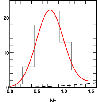
Figure 3: Distribution of absolute magnitudes for the clump stars closer than 50 pc from the sun. The observed distribution has been fitted using Eq. 2 giving $<\!M_{\rm v}\!>\,=\,0.74$ and $\sigma_{M_{\rm v}}\,=\,0.25$ for the local clump. The dashed line shows the contribution of field giants to the sample.

2.2.3 Construction of the sample

The local sphere sample is built using Hipparcos data where we select all stars with parallaxes larger than 5 mas (i.e. stars closer than 200 pc) in the same colour interval as the two NGP samples.

Then we correct the sample from Lutz-Kelker bias and we compare both corrections, first using the absolute magnitude correction (Eq. 3) and second using the distance correction (Eq. 4). The mean absolute magnitude correction of the sample is $-0.09$ mag with a standard deviation equal to 0.13 mag, and for the distances the mean correction is $-5.7$ pc with a standard deviation equal to 23.5 pc. Figure 5 shows the effect of the Lutz-Kelker bias on the luminosity function before and after correction. The continuous line gives the observed distribution in absolute magnitude, whereas the dashed line shows the corrected luminosity function. The sample defined by stars closer than 125 pc (537 stars) was then established using the corrected distances. The consistency has been checked by comparing the distance obtained after correction with Eq. 4 to the distance derived using the absolute magnitude correction. The difference in the two distances being of the order of 0.2 pc for the sample, this ensures us of the reliability of the correction.

We use the Barbier–Brossat & Figon (2000) catalogue that provides us with the radial velocities. We complete the sample with radial velocities from the Simbad database when measurements are existing. This leads to a nearly complete (98%) sample of 526 stars (out of 537 stars). Among those 526 stars, 27 have radial velocities from Simbad whereas 499 have radial velocities from Barbier–Brossat & Figon (2000).

Measurements errors for the radial velocities are given in two distinct ways in Barbier–Brossat & Figon (2000), either a value for $\sigma_{Vr}$ is given when available (224 stars) or a quality index (A to D) for stars whose radial velocities are obtained from a prism objective survey (275 stars). Figure 4 shows the distribution of errors of the radial velocity for stars with known $\sigma_{Vr}$ while Tab. 2 gives the distribution of the quality index for the stars with no $\sigma_{Vr}$.

Table 2: Distribution of the quality index for radial velocity of the stars of our sample in Barbier–Brossat & Figon (2000).

Quality Index		$\sigma_{Vr}$	(km/s)	number of stars
A		$\sigma_{Vr}$	$\leq$ 2.5	74
B	2.5 $<$	$\sigma_{Vr}$	$\leq$ 5.0	170
C	5.0 $<$	$\sigma_{Vr}$	$\leq$ 10.0	23
D	10.0 $\leq$	$\sigma_{Vr}$		8

Figure 4: Distribution of standard errors for the stars of the Hipparcos sample with given $\sigma_{Vr}$ in Barbier–Brossat & Figon (2000) (224 stars). 6 stars have errors larger than 5 km/s and are not within the limits of the plot.

Figure 5: Observed luminosity distribution (continuous line) versus the Lutz-Kelker bias corrected luminosity distribution (dashed line).

3 The force perpendicular to the Galactic plane and the disk mass distribution

Our first assumption is that stellar population distributions are in a stationary state with well mixed distribution functions according to coordinate z (distance from the Galactic plane) and w (vertical velocity). The second assumption is that the stellar motion separates in vertical and horizontal motions (separable potential), so the distribution function $f(z,w)$ of a tracer population depends only on the potential of the disk mass and on the kinetic energy of stars. For instance, it may be written as:

$$f(z,w)=\sum_{i=1}^{N}\frac{\rho_{i}(0)}{\sqrt{2\pi}\sigma_{w_{i}}}\exp\left[-\frac{\Phi(z)+\frac{w^{2}}{2}}{\sigma_{w_{i}}^{2}}\right]\mbox{,}$$ (5)

where $N$ is the number of isothermal disks, the $i^{th}$ population having the vertical velocity dispersion $\sigma_{w_{i}}$ and the local density $\rho_{i}(0)$. The vertical density of a stationary population is just:

$$\rho(z)=\sum_{i=1}^{N}\rho_{i}(0)\exp\left[-\Phi(z)/\sigma_{w_{i}}^{2}\right]=\sum_{i=1}^{N}\rho_{i}(z)\mbox{.}$$ (6)

This second assumption is valid as long as the analysed sample covers a restricted range of distances close to the Galactic plane like the bulk of our NGP stars between 162 pc and 870 pc. At higher distances, the potential cannot be considered as separable in $r$ and $z$ and the inclination of the velocity ellipsoid must be included in the analysis: see for instance Kuijken and Gilmore (1989) and Statler (1989).

The vertical potential (Kuijken and Gilmore 1989) is written

$$\Phi(z)=2\pi G(\Sigma_{0}(\sqrt{z^{2}+D^{2}}-D)+\rho_{\rm eff}z^{2})$$ (7)

a 3-parameter ($D$, $\Sigma_{0}$, $\rho_{\rm eff}$) representation to study the shape of the vertical potential. Another approach consists in building a stellar disc mass model and in considering that supplementary mass (unidentified mass) is proportional to the disc mass model or to one of its sub-component (see for instance Bahcall (1984); Holmberg & Flynn (2000)).

The total vertical mass distribution is deduced from $\Phi(z)$ through the Poisson equation and discussed in many papers (von Hoerner (1960); for extensive references see Crézé et al. (1998a); Holmberg & Flynn (2000), they also discuss the horizontal potential contribution to the dynamical estimate of the disk mass).

We derive the potential parameters as well as the stellar sample distributions (through the $\rho_{i}$ and $\sigma_{w_{i}}$) by using a maximum likelihood method. The maximum likelihood method allows the fit without binning of data. It allows a non-biased estimate of parameters even when the number of objects in bins would be small and the fluctuations are not gaussian and the use of a least square fitting would not be justified. Theoretical bases for this scheme can be found for instance in Kendall & Stuart (1973) or in Eadie et al. (1971).

We set $f^{*}(x_{i})$ the probability function of observables $x_{i}$ whose detailed expression is given below.

The logarithm of the likelihood is then defined as:

$$\log L=\sum_{i=1}^{n*}\log f^{*}(x_{i})\mbox{,}$$ (8)

where $n*$ is the number of red clump stars in the whole sample. We have separated the fields in subsamples according to distance and/or magnitude completeness. Then each subsample requires a specific treatment and $f^{*}$ has a different detailed algebrical expressions. It may be however written as:

$$f^{*}=\frac{{\cal M}_{1}+{\cal M}_{2}+{\cal M}_{3}}{{\cal N}_{1}+{\cal N}_{2}+{\cal N}_{3}}$$

where the ${\cal M}_{i}$ are the distribution function in the volume $V_{i}$ expressed in the used observable variables, and the ${\cal N}_{i}$ are their normalizations over each volume $V_{i}$. The ${\cal M}_{i}$ and ${\cal N}_{i}$ are explicited in the following subsections according to the type of completeness.

We have determined the model parameters using different observables $(z,r,b,w,m_{\rm v},\textrm{or\leavevmode\nobreak\ }M_{\rm V})$ in order to find the most efficient and accurate way to analyse the samples. Model with a simple limit ($z$-distance) have a simple algebra and are easier to develop. Models using supplementary stars ($r$-distance or magnitude completeness) would be more accurate, they have also more complicated algebra. We compare the numerical consistency of the various methods and check the most efficient and accurate ones.

Observations are available in three volumes ${\bf V}_{k}$, the two cones towards the NGP ($k=1,2$) and the local sphere ($k=3$). The number density of the stars is, according to the dynamical model:

$${\rm d}N(x,y,z,w)=\begin{cases}f(z,w)\,{\rm d}x{\rm d}y{\rm d}z{\rm d}w\\ 0\textrm{\leavevmode\nobreak\ \leavevmode\nobreak\ if $(x,y,z,w)$ is outside {\bf V${}_{k}$}}\end{cases}$$

or in galactic coordinates:

$${\rm d}N(r,l,b,w)=\begin{cases}f(r\sin(b),w)\,r^{2}\cos(b)\,{\rm d}r{\rm d}b{\rm d}l{\rm d}w\\ 0\textrm{\leavevmode\nobreak\ \leavevmode\nobreak\ if $(r,l,b,w)$ is outside {\bf V${}_{k}$}}\end{cases}$$

Due to the extended angular size of the observed NGP fields, the dependence on Galactic latitude ${\it b}$ cannot be neglected and, by comparison to traditional studies, makes the algebra more tedious.

3.1 Local sphere

The sample extracted from Hipparcos data and corrected for Lutz-Kelker bias defines a volume that is complete in distance. This volume $V_{k=3}$ is a sphere of radius $R_{s}=125$ pc.

The stellar density according to variables $z$ and $w$ is modelled as:

$${\rm d}{\cal N}_{3}(z,w)=\begin{cases}\int_{l}\int_{b}{\rm d}N=f(z,w)\,\pi\,(R_{s}^{2}-z^{2})\,{\rm d}z{\rm d}w\\ 0\text{\leavevmode\nobreak\ \leavevmode\nobreak\ if\leavevmode\nobreak\ }|z|>R_{s}\end{cases}$$

We have ${\cal M}_{3}={\rm d}{\cal N}_{3}/({\rm d}z{\rm d}w)$ and

$${\cal N}_{3}=\int_{V_{3}}{\rm d}N=\Sigma_{i}\int_{z}\rho_{i}(z)\,\pi\,(R_{s}^{2}-z^{2})\,{\rm d}z$$

3.2 NGP: completeness in $z$–distances

We have used the largest cone samples towards the NGP that are complete in $z$ height above the Galactic plane. For field 1, the volume $V_{1}$ is limited in $z$ between 226 and 391 pc (309.4 square degree field) and for field 2, between 226 and 579 pc (410.1 square degree field).

We have with $k=1,2$:

$${\rm d}{\cal N}_{k}(z,w)=\begin{cases}\left(\int\left[\frac{1}{2(\sin b)^{2}}\right]_{b_{\rm low}}^{b_{\rm up}}{\rm d}l\right)f(z,w)\,z^{2}{\rm d}z{\rm d}w\\ 0\textrm{\leavevmode\nobreak\ \leavevmode\nobreak\ outside of the volume {\bf V}${}_{k}$ }\end{cases}$$

where $b_{\rm low}$ and $b_{\rm up}$ are the lower and upper latitude boundaries at fixed longitude. We have ${\cal M}_{k}={\rm d}{\cal N}_{k}/({\rm d}z{\rm d}w)$, and

$${\cal N}_{k}\!=\!\int_{V_{k}}\!{\rm d}N\!=\!\left(\int\left[\frac{1}{2(\sin b)^{2}}\right]_{b_{\rm low}}^{b_{\rm up}}\,{\rm d}l\right)\!\left(\Sigma_{i}\int\rho_{i}(z)\,z^{2}{\rm d}z\right)$$

Integrals can be separated since the $l$ and $b$ contours do not depend on $z$, according to the definition of the sub-samples.

3.3 NGP: completeness in $r$–distances

To increase the number of stars used to constrain the model, we define complete volumes in distance from the sun, $r$. For volume $V_{1}$, $r$ range from 226 to 405 pc and for volume $V_{2}$, $r$ range from 226 to 616 pc.
We have with $k=1,2$:

$${\rm d}{\cal N}_{k}(b,r,w)=\begin{cases}\int_{l}{\rm d}N=\Delta l(b)\leavevmode\nobreak\ f(z,w)\,r^{2}\cos(b){\rm d}r{\rm d}b{\rm d}w\\ 0\text{\leavevmode\nobreak\ \leavevmode\nobreak\ outside of the volume {\bf V}${}_{k}$}\end{cases}$$

we define ${\cal M}_{k}={\rm d}{\cal N}_{k}/({\rm d}r{\rm d}b{\rm d}w)$, and

$${\cal N}_{k}=\int_{Vi}{\rm d}{\cal N}_{k}=\Sigma_{i}\int_{b}\Delta l(b)\int_{r}\rho_{i}(z)\,r^{2}\cos(b){\rm d}r{\rm d}b$$

In the previous equations, since the distribution function $f$ is independent of $l$, the $\Delta l(b)$ term, which is the longitude interval at latitude $b$ of a circular field, has a closed form given by solving ${\bf r}\cdot{\bf r}_{c}=\cos(\alpha)$, where $\alpha$ is the radius of the field, ${\bf r}_{c}$ the unit vector pointing towards the center of the field and ${\bf r}$ a unit vector. With $l_{c}$ and $b_{c}$ the coordinates of the center of the field and $\alpha$ its radius, we obtain the expression valid for the field 1:

$$\Delta l(b)=2\arccos\left(\frac{\cos(\alpha)-\sin(b)\sin(b_{c})}{\cos(b)\cos(b_{c})}\right)\,\mbox{.}$$

For the field 2, $\Delta l(b)$ is $2\pi$ since the field is centred toward the Galactic pole, unless the latitude $b$ corresponds to the removed area of the Coma Berenices cluster or to the field 1 overlapping region. Since these removed region are circular, we have:

$$\Delta l(b)=2\pi-\Delta_{coma}l(b)-\Delta_{field\,1}l(b)\,\,\mbox{.}$$

3.4 NGP: apparent magnitude completeness

Since the NGP samples have been selected by apparent magnitude, it is more efficient, in terms of the number of stars used, to keep this criterion. Modelling the distribution of apparent magnitudes of selected clump stars allows the use of 201 stars from 160 to 870 pc from the Galactic plane.
With $k=1,2$, we have:

$${\cal M}_{k}={\rm d}{\cal N}_{k}(b,m_{\rm v},w)/({\rm d}b{\rm d}m_{\rm v}{\rm d}w)=$$

$$\leavevmode\nobreak\ \leavevmode\nobreak\ \begin{cases}=\Delta l(b)\int_{r=0}^{\infty}f(r\sin(b),w)\Phi(M_{\rm V})\,r^{2}\cos(b)\,{\rm d}r\\ \textrm{or\leavevmode\nobreak\ }=0\textrm{\leavevmode\nobreak\ \leavevmode\nobreak\ if\leavevmode\nobreak\ }m_{\rm v}\,\textrm{is outside the limits given in Table\,\ref{t:samples}}\end{cases}$$

where $\Delta l(b)$ has been previously defined. We have also:

$${\cal N}_{k}\!=\!\Sigma_{i}\!\int_{b}\!\Delta l(b)\int\!\!\int\rho_{i}(r\sin(b))\Phi(M_{\rm V})\,r^{2}\cos(b)\,{\rm d}r{\rm d}b{\rm d}m_{\rm v}$$

3.5 NGP: apparent magnitude completeness (with absolute magnitudes and distances)

We use the same selection criterion in apparent magnitudes, with 200 stars in the range 200–750 pc from the Galactic plane.
Here we model both the distributions of absolute magnitudes and distances expecting a more constraining use of the observables $M_{\rm V}$
We have with $k=1,2$

$${\cal M}_{k}={\rm d}{\cal N}_{k}(z,b,w,M_{\rm V})/({\rm d}r{\rm d}b{\rm d}w{\rm d}M_{\rm V})=$$

$$\leavevmode\nobreak\ \leavevmode\nobreak\ \begin{cases}=\Delta l(b)f(z,w)\Phi(M_{\rm V})r^{2}\cos(b)\\ \textrm{or\leavevmode\nobreak\ }=0\textrm{\leavevmode\nobreak\ \leavevmode\nobreak\ if\leavevmode\nobreak\ }m_{\rm v}\,\textrm{is outside the limits given in Table\,\ref{t:samples}}\end{cases}$$

and we have:

$${\cal N}_{k}\!=\!\Sigma_{i}\!\!\int_{b}\!\!\Delta l(b)\!\!\int_{r}\,\int_{M_{\rm V}}\!\!\!\rho_{i}(r\sin(b))\Phi(M_{\rm V})\,r^{2}\!\!\cos(b)\,{\rm d}r{\rm d}M_{\rm V}{\rm d}b$$

4 Results

Modelling.

The modelling of the samples consists in reproducing the distribution of the observed apparent magnitudes, absolute magnitudes, distances and vertical velocities by adjusting the three vertical potential parameters (the total surface mass density $\Sigma_{0}$, the mass scale height $D$, and the halo local effective mass density $\rho_{\textrm{eff}}$) as well as the stellar density and velocity distributions (through the velocity dispersions and the respective contribution of each isothermal component). Using the four methods previously described, the model parameters are adjusted by a maximum likelihood. The maximum likelihood method avoids bias that would be introduced by a binning of data and by the small size of our samples. As expected, the accuracy is better with methods using more stars and/or more distant stars, while the comparison of methods allows to check their respective robustness. Following discussions are based on the results given by methods number 3 and 4.

$\rho_{\textrm{eff}}$.

The parameter $\rho_{\textrm{eff}}$ is introduced to model the local contribution of a spherical massive halo. A realistic range for this parameter is 0 to 0.02 M_⊙ pc^-3 (Kuijken and Gilmore 1989). However, this halo contribution to the vertical potential is quadratic in $z$ (at small $z$) and cannot be clearly distinguished from the disk contribution (the remaining terms in Eq. 7) that is also quadratic for small $z$. For these reasons, $\rho_{\textrm{eff}}$ is set at $0.01$ M_⊙ pc^-3.

Adjusted parameters.

The best decomposition of the observed stellar distributions in kinematic components, using methods 3 or 4, is obtained with three isothermal components with densities (22%, 59% and 19%) and respective vertical velocity dispersions $\sigma_{w}$ (8.5, 11.4 and 31.4) km s^-1. A two-component decomposition gives nearly the same likelihood with respective densities (78% and 22%) and vertical velocity dispersions (12.0 and 30.4) km s^-1. This result can be compared to the kinematic decomposition obtained in paper I (Soubiran et al 2002) using the 3D velocity components and the metallicity.

The maximum of likelihood gives also the following result: with method 3 ($D$, $\Sigma_{0}$)= (492 pc, 72 M_⊙ pc^-2) and with method 4 ($D$, $\Sigma_{0}$)= (1500 pc, 193 M_⊙ pc^-2). At a 1-$\sigma$ error level methods 3 and 4 give only a lower limit for $D$ respectively 227 pc and 400 pc and no upper limit. The $\Sigma_{0}$ values are strongly correlated with $D$ (see Figure 6). We must consider that our sample puts lower limits to ($D$, $\Sigma_{0}$) parameters and a sample with higher $z$-distances would be needed to put upper limits.

If $D$ were known independently, the relative accuracy on $\Sigma_{0}$ would be 12 %, while considering the seven model parameters (including dispersions and relative density of the two stellar components, $D$ and $\Sigma_{0}$), we find a large correlation between the two parameters $D$ and $\Sigma_{0}$. We may note that we obtain the first direct observational constraint on the thickness of the total disk mass. We also obtain a constraint on the total local mass density $\rho_{\rm{total}}$(z=0)=0.08$\pm$0.01 M_⊙ pc^-3 (see below).

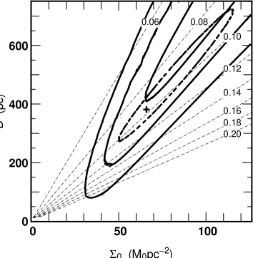
Figure 6: 1, 2 and 3–$\sigma$ error contours for $\Sigma_{0}$ and $D$ solutions obtained with method 4 (continuous curves). Using also the recent Oort limit determination 0.0102 M_⊙ pc^-3 from (Holmberg & Flynn 2000) gives better constraints (1–$\sigma$ error level: dashed curve). Dashed–dotted lines show solutions for adopted local mass density $\rho_{\rm total}$ values between 0.06 to 0.2 $\mathrm{M}_{\odot}\mathrm{pc}^{-3}$.

Comment about $D$.

In some previous vertical Galactic force determinations, simplifying assumptions have been adopted concerning the exact shape of the vertical mass distribution. For instance, Kuijken and Gilmore (1989) modelled the potential using Eq. 7, but assuming $D$ = 180 pc. They argue that their result is not sensitive to a small change on $D$ since the majority of their sample ranges beyond 500 pc from the Galactic plane. However since a significant fraction of their sample ranges between 200 and 500 pc, we suspect, that with a drastic change of $D$ at $\sim$500 pc, their data would be fitted with a higher $\Sigma_{0}$ value. Other previous determinations of the total surface mass density, based on one parameter models for the potential, could suffer a similar bias.

Table 3: $\Sigma_{0}$ and $D$ solutions for the potential within 1–$\sigma$ error and associated total local mass density and column density.

$\Sigma_{0}$	$\mathrm{M}_{\odot}\mathrm{pc}^{-2}$	64.	90.	193.
$D$	pc	400	637	1500
$\rho_{\rm eff}$	$\mathrm{M}_{\odot}\mathrm{pc}^{-3}$	0.01	0.01	0.01
$\rho_{\rm total}(0)$	$\mathrm{M}_{\odot}\mathrm{pc}^{-3}$	0.090	0.081	0.074
$\Sigma(800$ pc)	$\mathrm{M}_{\odot}\mathrm{pc}^{-2}$	73.2	86.4	106.8
$\Sigma(1.1$ kpc)	$\mathrm{M}_{\odot}\mathrm{pc}^{-2}$	82.2	99.9	136.1

Figure 7: Left : vertical force in (km/s)²/pc for the three solutions within 1–$\sigma$ presented in Tab. 2. Right : associated stellar density in log (M_⊙ pc^-3).

Total local mass density $\rho_{\rm{total}}$(z=0).

A set of $\Sigma_{0}$ and $D$ solutions within 1–$\sigma$ error are given in Table 2 with their corresponding total local mass volume density $\rho_{\rm{total}}(z=0)$ (according to Eq. 7 the local mass density is given by $\rho_{\rm{total}}(z=0)=\Sigma_{0}/(2D)+\rho_{\rm{eff}}$). We also give the total mass density within 800 pc from the Galactic plane including the halo contribution parametrized with $\rho_{\rm eff}$ (our surface mass density determination applies only up to $\sim$ 800 pc, the limit of our sample). The acceptable range of values for $\Sigma_{0}$ and $D$ is large, resulting in a wide range of possible mass distributions. This can be seen on the left panel of figure 7 where are plotted the $K_{z}$ solutions given in Tab 2 (recall that $K_{z}$ is proportional to $\Sigma(z)$) .

To disentangle the different solutions, we need more observations in the range 750 pc to 1.1 kpc. This is illustrated on the right panel of Fig. 7 by the predicted clump giant density (the observable quantity), where we can see that the solutions quoted in Tab. 3 differ significantly above 750 pc.

We may remark that the total local mass density $\rho_{\rm{total}}(z=0)$ given in Table 2 ranges below 0.10 $\mathrm{M}_{\odot}\mathrm{pc}^{-3}$ and is in agreement with recent and independent determinations based on Hipparcos data, compatible with local mass density of known matter.

Additional constraint from $\rho_{\rm total}(z=0)$: the Oort limit.

In Table 2, the different solutions differ by their predicted total volume mass density, from 0.07 to 0.09  M_⊙ pc^-2 but remain in agreement with the recent measures of $\rho_{\rm{total}}$($z$=0) based on Hipparcos data (Crézé et al. 1998a, b; Pham 1998; Holmberg & Flynn 2000) ranging from 0.076 to 0.102 $\mathrm{M}_{\odot}\mathrm{pc}^{-3}$.

The data set of clump giants that we have used does not allow to constrain more efficiently the local volume mass density $\rho_{\rm total}(z=0)$. Most of the constraints would come from the local sample within 125 pc, but due to the high velocity dispersions of the red giant stars, their density distribution is nearly uniform within 125 pc and the bending of the vertical density distribution due to the potential cannot be measured significantly. We notice that the analysis of red clump stars in a sphere of 250 pc would help to constrain the local volume density since they have distances measured by Hipparcos but they have no measured or published radial velocities. This would give a new independent determination, however the amplitude of the Lutz-Kelker or Malmquist bias will be large and certainly difficult to model properly.

So we consider the recent results based on Hipparcos data of the local volume mass density $\rho_{\rm{total}}$($z$=0). Differences on $\rho_{\rm{total}}$($z$=0) between Crézé et al. (1998a) and Holmberg & Flynn (2000) are within 1–$\sigma$ and are explained by Holmberg & Flynn (2000) as due to different assumptions on the exact shape of the potential. Crézé et al. (1998a) assume a quadratic potential close to the Galactic plane while Holmberg & Flynn (2000) suppose that the vertical potential is proportional to a more realistic model of the vertical stellar disk distribution. Admitting this more realistic hypothesis for the shape of the potential, we consider that Hipparcos data gives $\rho_{\rm{total}}(z=0)$   =   0.102   $\pm$   0.010   M_⊙  pc^-3 (Holmberg & Flynn 2000) and combining this result and our result obtained from distant red clump giants, we deduce stronger constraints on $\Sigma_{0}$ and $D$ (Figure 6: dashed contour draws the 1-$\sigma$ limit). We deduce that the scale height $D$ is relatively large, $390^{+330}_{-120}$ pc, as well as the total surface mass density $\Sigma_{0}$ = 67 ${}^{+47}_{-18}\,\mathrm{M}_{\odot}\mathrm{pc}^{-2}$, and the mass within 800 pc is $\Sigma$($|z|<$800 $\rm{pc})$ = 76${}_{-12}^{+25}\,\mathrm{M}_{\odot}\mathrm{pc}^{-2}$. The quantity $\Sigma$($|z|<$1100 $\rm{pc})$ = 85${}_{-13}^{+32}\,\mathrm{M}_{\odot}\mathrm{pc}^{-2}$ can be directly compared to the result obtained by Kuijken and Gilmore (1991) : $\Sigma$($|z|<$1100 $\rm{pc})$ = 71$\pm 6\,\mathrm{M}_{\odot}\mathrm{pc}^{-2}$. The two results are compatible in the 1$\sigma$ limit but our error bars are very large due to the poor constraint on $D$. The agreement between the maximum likelihood solution and the data is shown in figure 8. The NGP sample exhibits an offset of the $w$ velocity towards more negative values than the expected -7 km/s due to solar motion. This offset is visible at all distances, however its increase with $z$ is doubtful. We have to consider that a negative offset is a real feature in the data because our $w$ velocities have an accuracy better than 1 km/s due to the contribution of the ELODIE radial velocities by more than 94% in the considered direction. Nevertheless, this offset is not constant and is therefore not accounted for in the modeling. Table 4 shows the mean value of $w$, standard deviation and standard error on mean W for various intervals in $z$.

Figure 8: Predicted counts for our best fit model of the vertical potential (solid line) compared to the observed distribution (histogram). Top : Hipparcos sample. Middle : NGP sample of radius 15^∘. Bottom : NGP sample of radius 10^∘. Left : cumulative distribution of $z$ distance (Hipparcos sample) or $V_{j}$ (NGP samples). Right : distribution of vertical velocities. The dashed and dotted lines are the contribution of each isothermal population.

Table 4: $w$ behaviour as a function of $z$.

$z$ interval		number of stars	$<w>$	standard deviation	mean error
-125	0	252	-7.8	18.4	1.2
0	125	270	-7.9	17.1	1.1
125	250	30	-13.8	11.7	2.1
250	375	46	-12.4	22.5	3.3
375	500	56	-7.7	27.9	3.7
500	625	64	-15.5	26.4	3.3
625	750	52	-9.3	31.6	4.4

5 Discussion

With samples of giants in the solar neighbourhood up to distances of 800 pc toward the NGP, we solve for the vertical Galactic potential and the total disk surface mass density at the solar Galactic position.

We find a vertical potential $\Phi(z)$ compatible at high $z$ ($\sim$ 400–800 pc) with previous estimates (Kuijken and Gilmore 1991; Flynn & Fuchs 1994). We are also able to measure for the first time, the thickness of the total disk mass distribution, and find a characteristic height $D$=390 pc with a 1–$\sigma$ range from 271 pc to 720 pc.

This scale height $D$ corresponds to a 350 pc scale height of a vertically exponential density law in the range of $z$-height 200 to 500 pc. Figure 9 shows also the resulting total mass density from Eq. 7 and the stellar density for two exponential disks (old and thick disks respectively with 350 pc and 750 pc scale heights and a relative density of 15 per cent). This measure of the mass scale height is in agreement with the recent determination of the stellar disk scale height, h_z=330 pc, by Chen et al. (2001) based on SDSS star counts and compatible with lower estimates from star counts (for instance $260$ $\pm$ 50 pc by Ojha et al. (1996), 250 $\pm$ 60 pc by Vallenari et al. (2000) or 260 $\pm\,90\,$pc by Sohn (2002)). Below $z$=600 pc, the contribution of the stellar thick disk remains always much smaller than the old disk, and beyond 600 pc its contribution remains smaller than the dark halo (see Figure 9).

Figure 9: Vertical distribution of the volume mass density in the Galactic disk deduced from our dynamical determination (continuous line). A disk vertically exponential with a 350 pc scale height (dotted line), and complemented with a thick disk (scale height 750 pc, and relative density of 15 % at $z$=0 (dashed line).

We find for the surface mass density within 800 pc from the Galactic plane a value of $\Sigma$(800 pc)= 76 $\mathrm{M}_{\odot}\mathrm{pc}^{-2}$ (this value includes the contribution from known or “seen” matter -stellar and gas- and a contribution from a round massive dark halo) and we find for the total disk surface mass density $\Sigma_{0}$= 67 $\mathrm{M}_{\odot}\mathrm{pc}^{-2}$. This disk with a round dark halo (with a local density $\sim$0.01$\mathrm{M}_{\odot}\mathrm{pc}^{-3}$) may produce the observed flat rotation curve. Modellings with similar parameters can be found in Kuijken and Gilmore (1991) and Crézé et al. (1998a).

Our 1-$\sigma$ error upper limit allows a maximum $\Sigma_{0}$ = 114 $\mathrm{M}_{\odot}\mathrm{pc}^{-2}$ and a scale height of 720 pc. It is about the upper limit $\sim 100\,\mathrm{M}_{\odot}\mathrm{pc}^{-2}$ putting all the Galactic mass in the disk (maximal disk) and still explaining the observed Galactic rotation curve (Sackett 1997). It would also imply that the dark matter is within a disk of about 1 kpc thickness. Such a flat dark matter has been rejected by some observational evidences: for instance on the basis of the observed coupling in the stellar 3D velocity distribution in the solar neighbourhood (Bienaymé 1999) implying a more or less round dark halo, or also on the non-precessing circular orbit of the Sagittarius tail around our Galaxy (Ibata et al. 2001) implying also that the halo is most likely spherical.

We conclude that the local volume mass density, the surface mass density of the disk are in agreement with our current knowledge of the known volume and surface density from gas and stellar components. Moreover, the thickness of the disk mass density distribution is compatible with the thickness of the stellar old disk.