Transfer of Polarized Radiation in Strongly Magnetized Plasmas and Thermal Emission from Magnetars: Effect of Vacuum Polarization

Abstract

We present a theoretical study of radiative transfer in strongly magnetized electron-ion plasmas, focusing on the effect of vacuum polarization due to quantum electrodynamics. This study is directly relevant to thermal radiation from the surfaces of highly magnetized neutron stars, which have been detected in recent years. Strong-field vacuum polarization modifies the photon propagation modes in the plasma, and induces a “vacuum resonance” at which a polarized X-ray photon propagating outward in the neutron star atmosphere can convert from a low-opacity mode to a high-opacity mode and vice versa. The effectiveness of this mode conversion depends on the photon energy and the atmosphere density gradient. For a wide range of field strengths, $7\times 10^{13}\mathrel{\raise 1.29167pt\hbox{$<$}\mkern-14.0mu\lower 2.58334pt\hbox{$\sim$}}B\mathrel{\raise 1.29167pt\hbox{$<$}\mkern-14.0mu\lower 2.58334pt\hbox{$\sim$}}{\rm a~{}few}\times 10^{16}$ G, the vacuum resonance lies between the photospheres of the two photon modes, and the emergent radiation spectrum from the neutron star is significantly modified by the vacuum resonance. (For lower field strengths, only the polarization spectrum is affected.) Under certain conditions, which depend on the field strength, photon energy and propagation direction, the vacuum resonance is accompanied by the phenomenon of mode collapse (at which the two photon modes become degenerate) and the breakdown of Faraday depolarization. Thus, the widely used description of radiative transfer based on photon modes is not adequate to treat the vacuum polarization effect rigorously. We study the evolution of polarized X-rays across the vacuum resonance and derive the transfer equation for the photon intensity matrix (Stokes parameters), taking into account the effect of birefringence of the plasma-vacuum medium, free-free absorption, and scatterings by electrons and ions.

1 Introduction

It has long been known that in a strong magnetic field even the vacuum has a nontrivial dielectric property; this is the result of vacuum polarization, a genuine quantum electrodynamics effect (Heisenberg & Euler 1936; Schwinger 1951; Adler 1971; Tsai & Erber 1975; Heyl & Hernquist 1997). This effect is usually negligible for $B\mathrel{\raise 1.29167pt\hbox{$<$}\mkern-14.0mu\lower 2.58334pt\hbox{$\sim$}}B_{Q}$, but becomes increasingly important when $B$ exceeds $B_{Q}$, where $B_{Q}=m_{e}^{2}c^{3}/(e\hbar)=4.414\times 10^{13}$ G is the magnetic field at which the electron cyclotron energy $\hbar\omega_{Be}=\hbar eB/(m_{e}c)$ equals $m_{e}c^{2}$. A number of studies in the late 1970s showed that vacuum polarization can affect radiative transfer in magnetized plasmas by modifying photon polarization modes and inducing features in the radiative opacities (Gnedin, Pavlov & Shibanov 1978a,b; Meszaros & Ventura 1978,1979; Pavlov & Shibanov 1979; Ventura, Nagel & Meszaros 1979; see Pavlov & Gnedin 1984 and Meszaros 1992 for review). These earlier studies were mostly applied to radio pulsars and accreting X-ray binaries, for which $B\mathrel{\raise 1.29167pt\hbox{$<$}\mkern-14.0mu\lower 2.58334pt\hbox{$\sim$}}B_{Q}$. Not surprisingly, the effect of vacuum polarization in these systems appears to be relatively minor and, as far as we know, no concrete observational manifestation of vacuum polarization has been identified.

In the last few years, soft gamma-ray repeaters (SGRs) and anomalous X-ray pulsars (AXPs) have been identified as a potentially new class of neutron stars (NSs) endowed with superstrong ($B\mathrel{\raise 1.29167pt\hbox{$>$}\mkern-14.0mu\lower 2.58334pt\hbox{$\sim$}}10^{14}$ G) magnetic fields, the so-called “magnetars” (see Thompson & Duncan 1996; Hurley 2000; Thompson 2001; Israel et al 2001). This has stimulated new studies on radiative processes in the superstrong magnetic field regime. Of particular relevance to the present paper is the detection of thermal X-rays from the surface of isolated magnetic NSs (see Pavlov et al. 2002 for a recent review), including five magnetar candidates (4 AXPs and one SGR; see, e.g., Patel et al. 2001; Juett et al. 2002; Tiengo et al. 2002). The thermal emission can potentially provide useful constraints on the interior physics, surface magnetic field and composition of NSs. Several recent works have begun to model the atmosphere emission from magnetars, including the effect of vacuum polarization (Bezchastnov et al. 1996; Bulik & Miller 1997; Özel 2001; Ho & Lai 2001, 2003; Lai & Ho 2002a; a review/comment of these works can be found in Ho & Lai 2003).

In a highly magnetized plasma which characterizes NS atmospheres, there are two photon polarization modes, and they have very different radiative opacities. Previous theoretical modeling of magnetic NS atmospheres (see Ho & Lai 2003 and references therein; see also Pavlov et al. 1995; Zavlin & Pavlov 2002 for reviews) are based on solving the transfer equations for the two photon modes. As we discuss and quantify in §2 and §3 below, this modal description of the radiative transport is, in general, inadequate to handle the vacuum polarization effect near the “vacuum resonance” where the modes can mix and even “collapse”. The main purpose of this paper is to clarify these issues and to derive general transfer equations that can be used to study the transport of polarized radiation in the superstrong field regime.

Section 2 contains a physical discussion of the vacuum polarization effect on radiative transfer in magnetized NS atmospheres. In §3, we derive the basic properties of photon modes in magnetized plasmas and quantify the limitation of the modal description of radiative transport. We then study in §4 and §5 the propagation of polarized photons in an inhomogeneous plasma. We derive in §6 the transfer equations for the photon intensity matrix and conclude in §7.

2 Vacuum Polarization Effect on Radiative Transfer and Atmosphere Spectra of Magnetars: A Physical Discussion

To motivate our quantitative study in §3-§6, we present a physical discussion of the effect of vacuum polarization on radiative transfer in strong magnetic fields and on the thermal spectra of magnetars (see Lai & Ho 2002a; Ho & Lai 2003; hereafter LH02 and HL03). This also serves to clarify some of the confusions that have appeared recently (see Lai & Ho 2002b).

In a highly magnetized NS atmosphere, both the plasma and vacuum polarization contribute to the dielectric property of the medium. A “vacuum resonance” arises when these two contributions “compensate” each other (Gnedin et al. 1978a,b; Pavlov & Shibanov 1979; Meszaros & Ventura 1979; Ventura et al. 1979). For a photon of energy $E$, the vacuum resonance occurs at the density

$$\rho_{V}\simeq 0.964\,Y_{e}^{-1}B_{14}^{2}E_{1}^{2}f^{-2}~{}{\rm g~{}cm}^{-3},$$ (1)

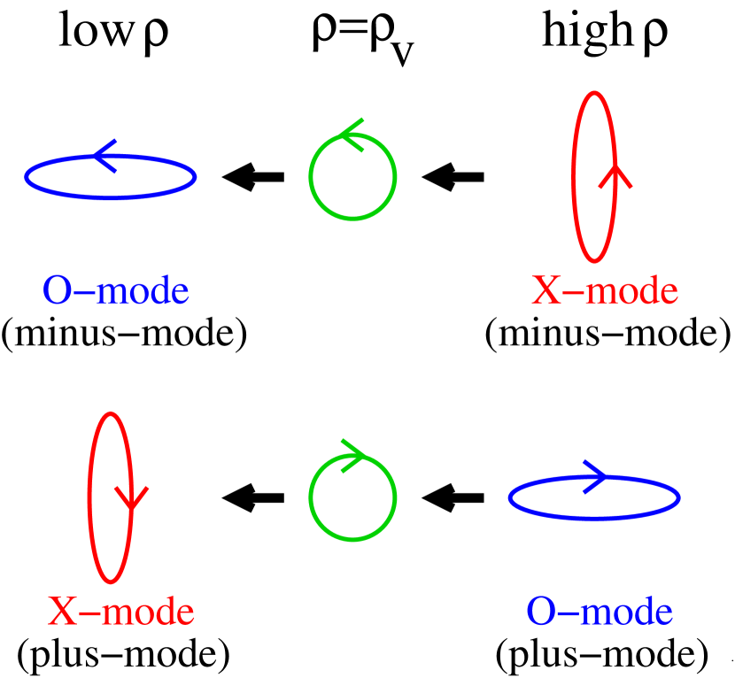
Figure 1: A schematic diagram illustrating mode conversion due to vacuum polarization: As a minus-mode (plus-mode) photon, which manifests as X-mode (O-mode) at high density (for $E>E_{Bi}$), traverses the vacuum resonance density $\rho_{V}$, it will stay as minus-mode (plus-mode) and become O-mode (X-mode) at low density if the adiabatic condition is satisfied (see also the left panels of Fig. 3). In this evolution, the polarization ellipse rotates $90^{\circ}$ and the photon opacity changes significantly.

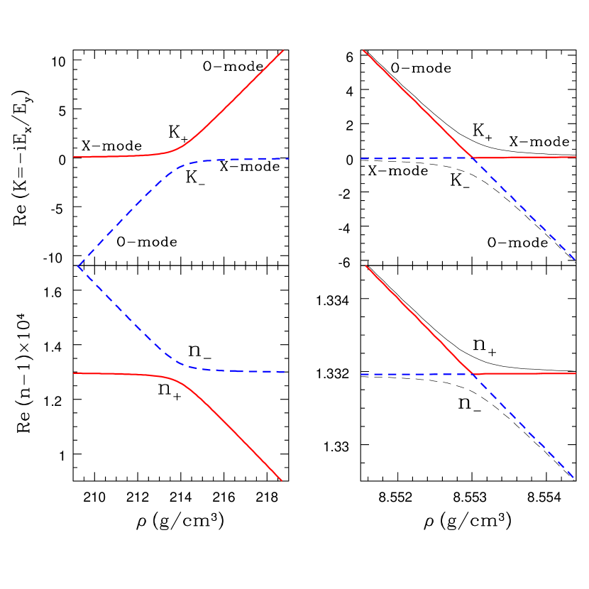
Figure 3: The polarization ellipticities $K$ [upper panels; see eq. (17)] and refractive indices (lower panels) of the photon modes as functions of density near vacuum resonance for $B=5\times 10^{14}$ G, $\theta_{B}=45^{\circ}$, and $Y_{e}=1$. The left panels are for $E=5$ keV, and the right panels for $E=1$ keV. On the right panels, the light curves show the results when damping is neglected, while the heavy lines include damping (we set $T=5\times 10^{6}$ K in evaluating $\gamma_{ei}$). On the left panels, the results are indistinguishable with and without damping. Note that the correspondence between the plus-, minus-modes and the X-, O-modes depends on the density and the photon energy ($E>E_{Bi}$ vs. $E<E_{Bi}$).

where $Y_{e}$ is the electron fraction, $E_{1}=E/(1~{}{\rm keV})$, $B=10^{14}B_{14}$ G is the magnetic field strength, and $f=f(B)$ is a slowly varying function of $B$ and is of order unity (LH02 and HL03). For $\rho>\rho_{V}$ (where the plasma effect dominates the dielectric tensor) and $\rho<\rho_{V}$ (where vacuum polarization dominates), the photon modes (for $E$ much smaller than the electron cyclotron energy $E_{Be}$) are almost linearly polarized (see Fig. 3 below): the extraordinary mode (X-mode) has its electric field vector ${\bf E}$ perpendicular to the ${\hat{\bf k}}$-${\hat{\bf B}}$ plane, while the ordinary mode (O-mode) is polarized along the ${\hat{\bf k}}$-$\hat{\bf B}$ plane (where ${\hat{\bf k}}$ specifies the direction of photon propagation, $\hat{\bf B}$ is the unit vector along the magnetic field). Near $\rho=\rho_{V}$, however, the normal modes become circularly polarized as a result of the “cancellation” of the plasma and vacuum effects — both effects tend to make the mode linearly polarized, but in mutually orthogonal directions. When a photon propagates in an inhomogeneous medium, its polarization state will evolve adiabatically if the density variation is sufficiently gentle. Thus, a X-mode (O-mode) photon will be converted into a O-mode (X-mode) as it traverses the vacuum resonance (see Fig. 1). This resonant mode conversion is analogous to the MSW effect of neutrino oscillation (e.g., Haxton 1995). For this conversion to be effective, the adiabatic condition must be satisfied:

$$E\mathrel{\raise 1.29167pt\hbox{$>$}\mkern-14.0mu\lower 2.58334pt\hbox{$\sim$}}E_{\rm ad}(B,\theta_{B},H_{\rho})$$

$$\qquad=1.49\,\bigl{(}f\,\tan\theta_{B}|1-u_{i}|\bigr{)}^{2/3}\left({5\,{\rm cm}\over H_{\rho}}\right)^{1/3}~{}{\rm keV},$$ (2)

where $\theta_{B}$ is the angle between ${{\hat{\bf k}}}$ and ${\hat{\bf B}}$, $u_{i}=(E_{Bi}/E)^{2}$, $E_{Bi}$ is the ion cyclotron energy, and $H_{\rho}=|dz/d\ln\rho|$ is the density scale height (evaluated at $\rho=\rho_{V}$) along the ray. For an ionized Hydrogen atmosphere, $H_{\rho}\simeq 2kT/(m_{p}g\cos\theta)=1.65\,T_{6}/(g_{14}\cos\theta)$ cm, where $T=10^{6}\,T_{6}$ K is the temperature, $g=10^{14}g_{14}$ cm s^-2 is the gravitational acceleration, and $\theta$ is the angle between the ray and the surface normal. We note that in this paper [as in our previous papers (LH02, HL03), and in several other references such as Meszaros & Ventura (1979), Meszaros (1992, p. 94), etc.], we refer to the O-mode as the mode with $|K|=|E_{x}/E_{y}|\gg 1$ and the X-mode as the mode with $|K|\ll 1$ (here the $z$-axis is along ${\hat{\bf k}}$ and the $y$-axis is in the direction of $\hat{\bf B}\times{\hat{\bf k}}$), thus the name “mode conversion”. Alternatively, one can define modes with definite helicity (the sign of $K=-iE_{x}/E_{y}$) such that $K$ changes continuously as $\rho$ changes; we call these plus-mode and minus-mode (see §3). Thus we may also say that in the adiabatic limit, the photon will remain in the same plus or minus branch, but the character of the mode is changed across the vacuum resonance. Indeed, in the literature on radio wave propagation in plasmas (e.g., Budden 1961; Zheleznyakov et al. 1983), the nonadiabatic case, in which the photon state jumps across the continuous curves, is referred to as “linear mode coupling”. It is important to note that the “mode conversion” effect discussed here is not a matter of semantics. The key point is that in the adiabatic limit, the photon polarization ellipse changes its orientation across the vacuum resonance, and therefore the photon opacity changes significantly . We prefer to use the term “mode conversion” since it captures this essential feature important for radiative transfer, and it is analogous to the MSW effect and other quantum mechanics problems involving adiabatic evolution of quantum states (Landau 1932; Zener 1932).

Because the two photon modes have vastly different opacities, the vacuum polarization-induced mode conversion can significantly affect radiative transfer in magnetar atmospheres. The main effect of vacuum polarization on the atmosphere spectrum can be understood as follows. When the vacuum polarization effect is neglected, the decoupling densities of the O-mode and X-mode photons (i.e., the densities of their respective photospheres) are approximately given by (for Hydrogen plasma) $\rho_{O}\simeq 0.42\,T_{6}^{-1/4}E_{1}^{3/2}G^{-1/2}$ g cm^-3 and $\rho_{X}\simeq 486\,T_{6}^{-1/4}E_{1}^{1/2}B_{14}G^{-1/2}$ g cm^-3 (see LH02), where $G=1-e^{-E/kT}$. The vacuum resonance lies between these two photospheres when $\rho_{O}<\rho_{V}<\rho_{X}$, i.e.

$$B_{l}<B<B_{h},$$ (3)

where

$$B_{l}\simeq 6.6\times 10^{13}\,f\,T_{6}^{-1/8}E_{1}^{-1/4}G^{-1/4}~{}{\rm G},$$ (4)

$$B_{h}\simeq 5.1\times 10^{16}\,f^{2}\,T_{6}^{-1/4}E_{1}^{-3/2}G^{-1/2}~{}{\rm G}.$$ (5)

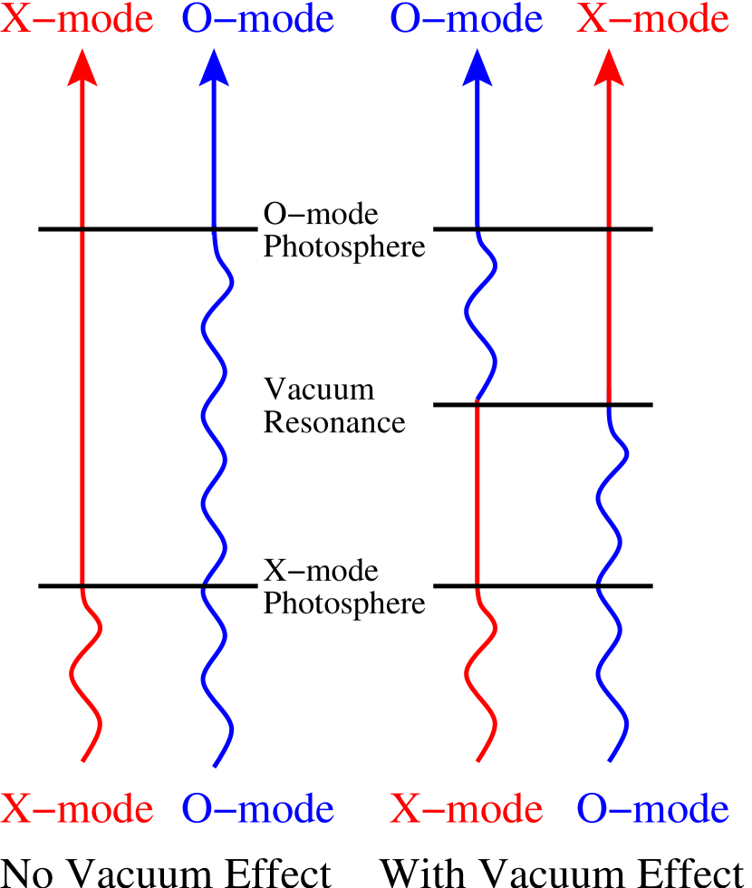
Figure 2: A schematic diagram illustrating how vacuum polarization-induced mode conversion affects radiative transfer in a magnetar atmosphere. When the vacuum polarization effect is turned off, the X-mode photosphere (where optical depth $\sim 1$) lies deeper than the O-mode. With the vacuum polarization effect included, the X-mode effectively decouples (emerges) from the atmosphere at the vacuum resonance, which lies at a lower density than the (original) X-mode photosphere.

When this condition is satisfied, the effective decoupling depths of the photons are changed. Indeed, we see from Fig. 2 that mode conversion makes the effective decoupling density of X-mode photons (which carry the bulk of the thermal energy) smaller, thereby depleting the high-energy tail of the spectrum and making the spectrum closer to black-body (although the spectrum is still harder than black-body because of nongrey opacities) . This expectation is borne out in self-consistent atmosphere modeling presented in HL03. Another important effect of vacuum polarization on the spectrum, first noted in HL03, is the suppression of proton cyclotron lines (and maybe other spectral lines; see also Ho et al. 2003). The physical origin for such line suppression is related to the depletion of continuum flux, which makes the decoupling depths inside and outside the line similar. HL03 suggests that the absence of lines in the observed spectra of several AXPs may be an indication of the vacuum polarization effect at work in these systems.

Our previous study (LH02) on the vacuum-induced mode conversion did not explicitly take into account of the effect of dissipation on the mode structure. Although this dissipative effect is small under many situations, near the vacuum resonance and for some directions of propagation, the two photon modes can “collapse”, i.e., they become identical and hence nonorthogonal (Soffel et al. 1983; see also Pavlov & Shibanov 1979). The analysis of LH02 breaks down near these “mode collapse” points (see §3). The question therefore arises as to how the polarization state evolves as the photon travels near the mode collapse point. Also, as mentioned in §1, previous studies of NS atmospheres with strong magnetic fields rely on the modal description of the radiative transport. This is valid only in the limit of large Faraday depolarization (Gnedin & Pavlov 1974), which is not always satisfied near the vacuum resonance especially for superstrong field strengths (see §3). More importantly, the transfer equations based on normal modes cannot handle the cases in which partial mode coupling (conversion) occurs across the vacuum resonance (i.e., when the adiabatic condition is neither strongly satisfied or violated). Clearly, to properly account for the effects of mode collapse, breakdown of Faraday depolarization, and mode conversion associated with vacuum polarization, one must go beyond the modal description of the radiation field by formulating and solving the transfer equation in terms of the photon intensity matrix (or Stokes parameters) and including the birefringence of the plasma-vacuum medium (see §5 and §6).

3 Photon Polarization Modes, Vacuum Resonance, Mode Collapse, and Faraday Depolarization

The property of photon modes in a magnetized electron-ion plasma including vacuum polarization was studied in LH02 and HL03 (see also Meszaros 1992 and references therein for earlier works in which electron plasmas with $B\ll B_{Q}$ were studied). In these papers, however, the damping terms in the dielectric tensor were largely neglected (but see §2.5 of HL03). Including these damping terms can (for certain parameter regimes) modify the mode property near the vacuum resonance and give rise to the phenomenon of mode collapse.

Following Ginzburg (1970), we consider a cold, magnetized plasma composed of electrons and ions (with charge, mass and number density given by $-e,~{}m_{e},~{}n_{e}$ and $Ze,~{}M=Am_{p},~{}n_{i}=n_{e}/Z$, respectively; here $Z$ is the charge number and $A$ is the mass number of the ion). The electrons and ions are coupled by collisions (with the collision frequency $\nu_{ei}$). We generalize Ginzburg’s result by including the radiative dampings of electrons and ions, with the damping frequencies $\nu_{re}$ and $\nu_{ri}$, respectively. In the coordinate system $XYZ$ with ${\bf B}$ along $Z$, the plasma contribution to the dielectric tensor is given by

$$\left[{\mbox{\boldmath$\epsilon$}}^{(p)}\right]_{{\hat{Z}}={\hat{B}}}=\left[\begin{array}[]{ccc}\varepsilon&ig&0\\ -ig&\varepsilon&0\\ 0&0&\eta\end{array}\right],$$ (6)

where

$$\hskip-22.76228pt\varepsilon\pm g\simeq 1-{v_{e}(1+i\gamma_{ri})+v_{i}(1+i\gamma_{re})\over(1+i\gamma_{re}\pm u_{e}^{1/2})(1+i\gamma_{ri}\mp u_{i}^{1/2})+i\gamma_{ei}^{\pm}},$$ (7)

$$\hskip-22.76228pt\eta\simeq 1-{v_{e}\over 1+i(\gamma_{ei}+\gamma_{re})}-{v_{i}\over 1+i(\gamma_{ei}+\gamma_{ri})}.$$ (8)

In eqs. (7) and (8), we have defined the dimensionless quantities

$$u_{e}={\omega_{Be}^{2}\over\omega^{2}},\quad u_{i}={\omega_{Bi}^{2}\over\omega^{2}},\quad v_{e}={\omega_{pe}^{2}\over\omega^{2}},\quad v_{i}={\omega_{pi}^{2}\over\omega^{2}},$$ (9)

where $\omega_{Be}=eB/(m_{e}c)$ is the electron cyclotron frequency, $\omega_{Bi}=ZeB/(Mc)=(Zm_{e}/Am_{p})\omega_{Be}$ is the ion cyclotron frequency, $\omega_{pe}=(4\pi n_{e}e^{2}/m_{e})^{1/2}$ is the electron plasma frequency, and $\omega_{pi}=(4\pi n_{i}Z^{2}e^{2}/M)^{1/2}=(Zm_{e}/Am_{p})^{1/2}\omega_{pe}$ is the ion plasma frequency. The dimensionless damping rates $\gamma_{ei}=\nu_{ei}/\omega$, $\gamma_{re}=\nu_{re}/\omega$, and $\gamma_{ri}=\nu_{ri}/\omega$ are given by

$$\gamma_{ei} = {Z^{2}n_{i}e^{4}\over\hbar\omega^{2}}\!\left({2\pi\over m_{e}kT}\right)^{1/2}\!\!\!(1-e^{-\hbar\omega/kT})\,g_{\alpha}^{\rm ff}$$ (10)

$$= 9.2\times 10^{-5}{Z^{2}\over A}{\rho_{1}\over T_{6}^{1/2}E_{1}^{2}}(1-e^{-E/kT})\,g_{\alpha}^{\rm ff},$$

$$\gamma_{re} = {2e^{2}\omega\over 3m_{e}c^{3}}=9.5\times 10^{-6}E_{1},$$ (11)

$$\gamma_{ri} = {Z^{2}m_{e}\over Am_{p}}\gamma_{re}=5.2\times 10^{-9}{Z^{2}\over A}E_{1},$$ (12)

where $g_{\alpha}^{\rm ff}$ is the Gaunt factor. In eq. (7),

$$\gamma_{ei}^{\pm}=\gamma_{ei}\left[1\mp u_{i}^{1/2}(1-Z^{-1})+m_{e}/(Am_{p})\right].$$ (13)

For Hydrogen plasmas, $\gamma_{ei}^{\pm}\simeq\gamma_{ei}$.

Including vacuum polarization, the dielectric tensor $\epsilon$ and inverse permeability tensor ${\mbox{\boldmath$\mu$}}^{-1}\equiv\bar{\mbox{\boldmath$\mu$}}$ can be written as ${\mbox{\boldmath$\epsilon$}}={\mbox{\boldmath$\epsilon$}}^{(p)}+\Delta{\mbox{\boldmath$\epsilon$}}^{(v)}$, $\bar{\mbox{\boldmath$\mu$}}={\bf I}+\Delta\bar{\mbox{\boldmath$\mu$}}^{(v)}$ (where ${\bf I}$ is the unit tensor). The vacuum corrections are

$$\Delta{\mbox{\boldmath$\epsilon$}}^{(v)}=(a-1){\bf I}+q\hat{\bf B}\hat{\bf B},$$ (14)

$$\Delta\bar{\mbox{\boldmath$\mu$}}^{(v)}=(a-1){\bf I}+m\hat{\bf B}\hat{\bf B},$$ (15)

where $a$, $q$, and $m$ are functions of $B$ (the explicit expressions are given in LH02 and HL03). Including the contribution from vacuum polarization, the dielectric tensor can still be written in the form of eq. (6), except

$$\varepsilon\rightarrow\varepsilon^{\prime}=\varepsilon+a-1,\qquad\eta\rightarrow\eta^{\prime}=\eta+a+q-1.$$ (16)

With the dielectric tensor and permeability tensor known, the photon modes can be determined in a straightforward manner. In the $xyz$ coordinates with ${\bf k}$ along the $z$-axis and lies in the X-Z plane (such that $\hat{\bf B}\times{{\hat{\bf k}}}=\sin\theta_{B}\,\hat{y}$, where $\theta_{B}$ is the angle between ${\bf k}$ and ${\bf B}$), we write the electric field of the mode as ${\bf E}_{\pm}\propto(iK_{\pm},1,iK_{z\pm})$, where the ellipticity $K_{\pm}=-iE_{x}/E_{y}$ is given by

$$K_{\pm}=\beta\pm\sqrt{\beta^{2}+r},$$ (17)

with $r=1+(m/a)\sin^{2}\theta_{B}\simeq 1$, and the (complex) polarization parameter $\beta$ is

$$\beta=-\frac{\varepsilon^{\prime 2}-g^{2}-\varepsilon^{\prime}\eta^{\prime}\left(1+m/a\right)}{2g\eta^{\prime}}\frac{\sin^{2}\theta_{B}}{\cos\theta_{B}}.$$ (18)

The refractive index $n_{\pm}$ is given by

$$n_{\pm}^{2}=\frac{g\eta^{\prime}}{a\epsilon_{33}}\left(\frac{\varepsilon^{\prime}}{g}+\frac{1}{K_{\pm}}\cos\theta_{B}\right),$$ (19)

where $\epsilon_{33}=\varepsilon^{\prime}\sin^{2}\theta_{B}+\eta^{\prime}\cos^{2}\theta_{B}$.

The polarization parameter $\beta$ directly determines the characteristics of photon normal modes in the medium. For $v_{e}\ll 1$, the real part of $\beta$ can be written as ${\rm Re}(\beta)=\beta_{0}\beta_{V}$, where

$$\beta_{0}\simeq\frac{u_{\rm e}^{1/2}\sin^{2}\theta_{B}}{2\cos\theta_{B}}\left(1-u_{\rm i}\right),$$ (20)

and

$$\beta_{V}\simeq 1+\frac{\left(q+m\right)\left(1-u_{\rm e}\right)}{u_{\rm e}v_{\rm e}}.$$ (21)

The condition ${\rm Re}(\beta)=0$ selects out three critical photon energies $E_{Be}=\hbar\omega_{Be},~{}E_{Bi}=\hbar\omega_{Bi}$ and $E_{V}$ (for a given density), where the latter is the vacuum resonance energy

$$E_{V}\simeq{\hbar\omega_{pe}\over\sqrt{q+m}}.$$ (22)

We shall concentrate on this vacuum resonance in the remainder of this paper. Since $E_{V}$ depends on density, a photon with a given energy $E$ traveling in an inhomogeneous medium encounters the vacuum resonance at the density $\rho_{V}$, given by eq. (1). Figure 3 show some examples of the mode properties near the vacuum resonance.

Including the damping terms in the dielectric tensor gives rise to the phenomenon of mode collapse (see Soffel et al. 1983 and references therein). This occurs when the two polarization modes become identical, i.e., $K_{+}=K_{-}$ or $n_{+}=n_{-}$, which requires $\beta=\pm i\sqrt{r}\approx\pm i$. Using eq. (18), we find, for $u_{e}\gg 1$, $v_{e}\ll 1$, and neglecting ions ($u_{i}\ll 1$),

$$\beta\approx\frac{u_{\rm e}^{1/2}}{2}\frac{\sin^{2}\theta_{B}}{\cos\theta_{B}}\left(\beta_{\rm V}-i\gamma_{\rm e}\right)$$ (23)

where $\beta_{\rm V}\approx 1-(q+m)/v_{\rm e}=1-(E/E_{\rm V})^{2}$ and $\gamma_{e}=\gamma_{ei}+\gamma_{re}$. So the condition $\beta=\pm i$ selects out a critical angle $\theta_{B}=\theta_{\rm coll}$ at which mode collapse occurs: $\sin^{2}\theta_{\rm coll}/\cos\theta_{\rm coll}=2/(u_{e}^{1/2}\gamma_{e})$. When the ion effect is included (i.e., when $u_{i}\mathrel{\raise 1.29167pt\hbox{$>$}\mkern-14.0mu\lower 2.58334pt\hbox{$\sim$}}1$), no simple expression for the complex $\beta$ can be obtained, and $\theta_{\rm coll}$ must be calculated numerically (see Fig. 4). Figure 4 shows that for “ordinary” field strengths ($B_{14}\mathrel{\raise 1.29167pt\hbox{$<$}\mkern-14.0mu\lower 2.58334pt\hbox{$\sim$}}0.1$), $\theta_{\rm coll}$ is very close to $90^{\circ}$ for most photon energies (in agreement with Soffel et al. 1983); for superstrong field strengths ($B_{14}\mathrel{\raise 1.29167pt\hbox{$>$}\mkern-14.0mu\lower 2.58334pt\hbox{$\sim$}}1$), however, $\theta_{\rm coll}$ can be much smaller than $90^{\circ}$. Figure 4 also shows that at $E=E_{Bi}$ (the ion cyclotron energy), the mode collapse point is always very close to $\theta_{B}=90^{\circ}$.

More generally, the modal description of radiative transfer is valid only in the limit of large Faraday depolarization, when the phase shift between the two modes over a mean free path is significant, i.e., when the condition $|\mbox{Re}(n_{+}-n_{-})|\gg|\mbox{Im}(n_{+}+n_{-})|$ is satisfied (Gnedin & Pavlov 1974). Consider first the situation where the ion effect is neglected (i.e., $u_{i}\ll 1$). For $u_{\rm e}\gg 1$, we find

$$\hskip-17.07182pt\mbox{Re}(n_{+}^{2}-n_{-}^{2}) \approx -{2v_{\rm e}\over u_{\rm e}^{1/2}}\cos\theta_{B}\mbox{Re}\left(\sqrt{1+\beta^{2}}\right),$$ (24)

$$\hskip-17.07182pt\mbox{Im}(n_{+}^{2}+n_{-}^{2}) \approx \gamma_{\rm e}v_{\rm e}\left[\sin^{2}\theta_{B}+{1\over u_{\rm e}}\left(1+\cos^{2}\theta_{B}\right)\right],$$ (25)

where $\beta$ is given by eq. (23). For $|\beta_{\rm V}|\gtrsim{\rm a~{}few}\times\gamma_{\rm e}$ (i.e., for $E$ slightly away from $E_{\rm V}$), we have $|{\rm Re}(n_{+}^{2}-n_{-}^{2})|\sim 2v_{e}u_{e}^{-1/2}{\rm max}(\cos\theta_{B},u_{e}^{1/2}\!\beta_{V}\sin^{2}\theta_{B})$, thus the condition for Faraday depolarization is satisfied for all $\theta_{B}$. On the other hand, for $|\beta_{\rm V}|\ll\gamma_{\rm e}$ (i.e., for $E$ extremely close to $E_{\rm V}$), the condition $|\mbox{Re}(n_{+}-n_{-})|\gtrsim|\mbox{Im}(n_{+}+n_{-})|$ requires $(\gamma_{\rm e}u_{\rm e}^{1/2}/2)|\sin^{2}\theta_{B}/\cos\theta_{B}|=|\mbox{Im}(\beta)|\lesssim 1$; this condition translates to $\theta_{B}\lesssim\theta_{\rm coll}$ or $\theta_{B}\gtrsim\pi-\theta_{\rm coll}$. In other words, the breakdown of Faraday depolarization at the vacuum resonance ($|\beta_{\rm V}|\ll\gamma_{\rm e}$) is restricted to an angular region of $\theta_{B}$ around $\pi/2$. For a given $B$ and $\theta_{B}$, to satisfy Faraday depolarization requires $E\gg E_{\rm Far}(B,\theta_{B})$, where $E_{\rm Far}(B,\theta_{B})$ is obtained by setting ${\rm Im}(\beta)=1$. This result can be generalized to the case where the ion effect is not negligible (i.e., $u_{i}\mathrel{\raise 1.29167pt\hbox{$>$}\mkern-14.0mu\lower 2.58334pt\hbox{$\sim$}}1$), although the simple expressions (24) -(25) are no longer valid. In general, while mode collapse at the vacuum resonance($\beta_{V}=0$) occurs only at two angles $\theta_{B}=\theta_{\rm coll}$ and $\pi-\theta_{\rm coll}$, the breakdown of Faraday depolarization occurs for $\theta_{\rm coll}\mathrel{\raise 1.29167pt\hbox{$<$}\mkern-14.0mu\lower 2.58334pt\hbox{$\sim$}}\theta_{B}\mathrel{\raise 1.29167pt\hbox{$<$}\mkern-14.0mu\lower 2.58334pt\hbox{$\sim$}}\pi-\theta_{\rm coll}$. To put it another way, for a given $B$ and $\theta_{B}$, there is a range of energies for which Faraday depolarization breaks down; we see from Fig. 5 that this range becomes larger as $B$ increases.

The above analysis shows that in the superstrong field regime ($B_{14}\mathrel{\raise 1.29167pt\hbox{$>$}\mkern-14.0mu\lower 2.58334pt\hbox{$\sim$}}1$), mode collapse and breakdown of Faraday depolarization at vacuum resonance can occur for a wide range of photon energies and propagation directions. Therefore, a rigorous treatment of radiative transfer near the vacuum resonance, in general, requires solving the transport equations for the four photon intensity matrix, or Stokes parameters.

4 Equations for the Evolution of Electromagnetic Waves and Mode Amplitudes

An electromagnetic (EM) wave with a given frequency $\omega$ satisfies the wave equation

$$\nabla\times(\bar{\mbox{\boldmath$\mu$}}\cdot\nabla\times{\bf E})={\omega^{2}\over c^{2}}\,{\mbox{\boldmath$\epsilon$}}\cdot{\bf E}.$$ (26)

We assume that the medium is weakly anisotropic so that deflection of the photon trajectory can be neglected. This requires that the deviation of $\epsilon$ or $\bar{\mbox{\boldmath$\mu$}}$ from the unit tensor is small. Consider a wave propagating in the $z$-direction. The external magnetic field is assumed to be constant, and the medium density varies in space with characteristic length scale $H_{\rho}\gg c/\omega$. Let ${\bf E}=e^{ik_{0}z}{\bf A}$, where $k_{0}\equiv\omega/c$. Assuming that $|d{\bf A}/dz|\ll k_{0}|{\bf A}|$ (geometric optics approximation), we have

$${dA_{x}\over dz}={ik_{0}\over 2a}\bigl{[}(\epsilon_{11}-a)A_{x}+\epsilon_{12}A_{y}+\epsilon_{13}A_{z}\bigr{]},$$ (27)

$${dA_{y}\over dz}={ik_{0}\over 2(a+m\sin^{2}\theta_{B})}\bigl{[}\epsilon_{21}A_{x}$$

$$\quad\qquad+(\epsilon_{22}-a-m\sin^{2}\theta_{B})A_{y}+\epsilon_{23}A_{z}\bigr{]},$$ (28)

$$~{}~{}A_{z}={\epsilon_{13}A_{x}+\epsilon_{23}A_{y}\over\epsilon_{33}},$$ (29)

where $\epsilon_{ij}$ is the component of the dielectric tensor in the $xyz$ coordinate system (with the $z$-axis along ${\bf k}$). We shall find that near the vacuum resonance, ${\bf A}$ can vary on the length scale $1/(k_{0}|n_{+}-n_{-}|)$ (see §5.2), much shorter than $H_{\rho}$, but the condition $|d{\bf A}/dz|\ll k_{0}|{\bf A}|$ is still easily satisfied as long as $|n_{+}-n_{-}|\ll 1$. Using the expressions for $\epsilon_{ij}$, we find that $|\epsilon_{13}/\epsilon_{33}|\simeq|(v_{e}-q)\sin\theta_{B}\cos\theta_{B}|$ and $|\epsilon_{23}/\epsilon_{33}|\simeq|v_{e}u_{e}^{-1/2}\sin\theta_{B}/(1-u_{i})|$ for $|u_{i}-1|\mathrel{\raise 1.29167pt\hbox{$>$}\mkern-14.0mu\lower 2.58334pt\hbox{$\sim$}}m_{e}/m_{p}$ (and $u_{e}\gg 1$). Thus, as long as $v_{e}\ll 1$ (valid for sufficiently low densities) and $q\ll 1$ (valid for $B_{14}\ll 600$), the wave is transverse for most photon energies (an exception occurs when $E$ is very close to $E_{Bi}$). We shall adopt this transverse approximation in the following . Since $a-1,~{}m\ll 1$, the evolution equation for ${\bf A}$ simplifies to

$${d\over dz}\left(\begin{array}[]{c}A_{x}\\ A_{y}\end{array}\right)={ik_{0}\over 2}\left[\begin{array}[]{cc}\sigma_{11}&\sigma_{12}\\ \sigma_{21}&\sigma_{22}\end{array}\right]\left(\begin{array}[]{c}A_{x}\\ A_{y}\end{array}\right)$$ (30)

where

$$\sigma_{11} = \epsilon_{11}-a=\varepsilon^{\prime}\cos^{2}\theta_{B}+\eta^{\prime}\sin^{2}\theta_{B}-a,$$ (31)

$$\sigma_{12} = -\sigma_{21}=\epsilon_{12}=ig\cos\theta_{B},$$ (32)

$$\sigma_{22} = \epsilon_{22}-a-m\sin^{2}\theta_{B}=\varepsilon^{\prime}-a-m\sin^{2}\theta_{B}.$$ (33)

Equation (30) can be used to study the evolution of EM wave amplitude across the vacuum resonance under the most general conditions. Equivalently, we can use the photon density matrix to study the wave propagation (§5).

4.1 Evolution of Mode Amplitude

It is instructive to show that when dissipation is neglected, eqs. (30) can be reduced to the evolution equations for the mode amplitudes given in LH02. Let

$$\left(\begin{array}[]{c}A_{x}\\ A_{y}\end{array}\right)=\exp\left[{ik_{0}\over 4}\int^{z}(\sigma_{11}+\sigma_{22})dz\right]\left(\begin{array}[]{c}{\cal A}_{x}\\ {\cal A}_{y}\end{array}\right).$$ (34)

Equations (30) reduce to

$${d\over dz}\left(\begin{array}[]{c}{\cal A}_{x}\\ {\cal A}_{y}\end{array}\right)={ik_{0}\Delta n\over 2}\left[\begin{array}[]{cc}\cos 2\theta_{m}&i\sin 2\theta_{m}\\ -i\sin 2\theta_{m}&-\cos 2\theta_{m}\end{array}\right]\left(\begin{array}[]{c}{\cal A}_{x}\\ {\cal A}_{y}\end{array}\right)$$ (35)

where $\Delta n$ is the difference of the indices of refraction for the two modes and $\theta_{m}$ is the “mixing angle”, as given by

$$\Delta n={-i\sigma_{12}\over\sin 2\theta_{m}},\quad\tan 2\theta_{m}={-2i\sigma_{12}\over\sigma_{11}-\sigma_{22}}.$$ (36)

When dissipation is neglected, $\Delta n$ and $\theta_{m}$ are real, and for $u_{e}\gg 1$, we find

$$\Delta n = -{v_{e}\cos\theta_{B}\over u_{e}^{1/2}(1-u_{i})\sin 2\theta_{m}},$$ (37)

$$(\tan 2\theta_{m})^{-1} = {u_{e}^{1/2}(1-u_{i})\sin^{2}\theta_{B}\over 2\cos\theta_{B}}\left(1-{q+m\over v_{e}}\right)$$ (38)

$$= \beta.$$

The normal mode eigenvectors are $({\cal A}_{x},{\cal A}_{y})=(i\cos\theta_{m},\sin\theta_{m})$ and $(-i\sin\theta_{m},\cos\theta_{m})$. We define the mode amplitude ${\cal A}_{+}$ and ${\cal A}_{-}$ via

$$\left(\begin{array}[]{c}{\cal A}_{x}\\ {\cal A}_{y}\end{array}\right)={\cal A}_{+}\left(\begin{array}[]{c}i\cos\theta_{m}\\ \sin\theta_{m}\end{array}\right)+{\cal A}_{-}\left(\begin{array}[]{c}-i\sin\theta_{m}\\ \cos\theta_{m}\end{array}\right).$$ (39)

The equations for the evolution of ${\cal A}_{+}$ and ${\cal A}_{-}$ are then given by

$$i{d\over dz}\left(\begin{array}[]{c}{\cal A}_{+}\\ {\cal A}_{-}\end{array}\right)=\left[\begin{array}[]{cc}-k_{0}\Delta n/2&i\,d\,\theta_{m}/dz\\ -i\,d\,\theta_{m}/dz&k_{0}\Delta n/2\end{array}\right]\left(\begin{array}[]{c}{\cal A}_{+}\\ {\cal A}_{-}\end{array}\right),$$ (40)

which agree with eq. (15) of LH02. Equations (35) and (40) have the standard forms of the level crossing problem in quantum mechanics (Landau 1932; Zener 1932). When

$$k_{0}\left|\Delta n\right|/2\gg\left|{d\,\theta_{m}/dz}\right|,$$ (41)

the polarization vector will evolve adiabatically (i.e., evolve along the continuous $K_{+}$ or $K_{-}$ curve). Evaluating this condition at vacuum resonance yields $E\gg E_{\rm ad}$ [see eq. (2) and LH02 for details]. In general, for a linear density profile, $\rho=\rho_{V}(1-z/H_{\rho})\simeq\rho_{V}\exp(-z/H_{\rho})$ (for $|z|\ll H_{\rho}$), the nonadiabatic jump probability is given by

$$P_{\rm jump}=\exp\left[-{(\pi/2)}\left(E/E_{\rm ad}\right)^{3}\right].$$ (42)

Thus, in practice, when $E\mathrel{\raise 1.29167pt\hbox{$>$}\mkern-14.0mu\lower 2.58334pt\hbox{$\sim$}}1.3\,E_{\rm ad}$, the evolution will be highly adiabatic (with $P_{\rm jump}\mathrel{\raise 1.29167pt\hbox{$<$}\mkern-14.0mu\lower 2.58334pt\hbox{$\sim$}}0.03$). Figure 6 shows the adiabatic regime $E>E_{\rm ad}$ in the $B$–$E$ plane for typical values of $\theta_{B}$ and $H_{\rho}$. [Another way to understand the adiabatic condition is discussed in §5.1; see eq. (60)].

5 Evolution of Stokes Parameters Across Vacuum Resonance

5.1 Evolution Equations for Photon Intensity Matrix

We now study the transfer equation for the photon intensity matrix, taking into account the birefringence of the plasma and the attenuation due to absorption and scattering; we relegate the derivation of the source functions to §6.

The intensity matrix $I_{\alpha\beta}$ of the radiation is defined as

$$I_{\alpha\beta}\equiv C\langle A_{\alpha}A_{\beta}^{\ast}\rangle,$$ (43)

where $\langle\cdots\rangle$ denotes time average ($\alpha,\beta=1,2$ or $x,y$). We choose the proportional constant $C$ such that $I_{\alpha\beta}$ has the units of specific intensity. The Stokes parameters $I,Q,U,V$ are related to $I_{\alpha\beta}$ via

$$\left[I_{\alpha\beta}\right]={1\over 2}\left[\begin{array}[]{cc}I+Q&U+iV\\ U-iV&I-Q\end{array}\right].$$ (44)

Using eq. (30), we can derive the evolution equation for the intensity matrix:

$${d\over dz}I_{\alpha\beta}=-{1\over 2}k_{0}\sum_{\gamma}\left(T_{\alpha\gamma}I_{\gamma\beta}+I_{\alpha\gamma}T_{\gamma\beta}^{+}\right),$$ (45)

where

$$T_{\alpha\beta}=-i\sigma_{\alpha\beta}.$$ (46)

Equivalently, the Stokes parameters ${\bf S}=(S_{0},S_{1},S_{2},S_{3})^{+}=(I,Q,U,V)^{+}$ evolve according to

$${d\over dz}\left(\begin{array}[]{c}I\\ Q\\ U\\ V\end{array}\right)=k_{0}\left[\begin{array}[]{cccc}T_{0}&T_{1}&T_{2}&T_{3}\\ T_{1}&T_{0}&-\Omega_{3}&\Omega_{2}\\ T_{2}&\Omega_{3}&T_{0}&-\Omega_{1}\\ T_{3}&-\Omega_{2}&\Omega_{1}&T_{0}\end{array}\right]\left(\begin{array}[]{c}I\\ Q\\ U\\ V\end{array}\right)$$ (47)

where

$$T_{0}=-{1\over 2}\left(\sigma_{11i}+\sigma_{22i}\right),$$ (48)

$$T_{1}=-{1\over 2}\left(\sigma_{11i}-\sigma_{22i}\right),$$ (49)

$$T_{2}=-{1\over 2}\left(\sigma_{12i}+\sigma_{21i}\right)=0,$$ (50)

$$T_{3}={1\over 2}\left(\sigma_{12r}-\sigma_{21r}\right)=\sigma_{12r},$$ (51)

$$\Omega_{1}={1\over 2}\left(\sigma_{11r}-\sigma_{22r}\right),$$ (52)

$$\Omega_{2}={1\over 2}\left(\sigma_{12r}+\sigma_{21r}\right)=0,$$ (53)

$$\Omega_{3}={1\over 2}\left(\sigma_{12i}-\sigma_{21i}\right)=\sigma_{12i}.$$ (54)

Here $\sigma_{\alpha\beta r}={\rm Re}(\sigma_{\alpha\beta})$ and $\sigma_{\alpha\beta i}={\rm Im}(\sigma_{\alpha\beta})$. Following Kubo & Nagata (1983), equation (47) can also be cast into a vector form. Define vectors in the Poincaré sphere

$${\bf s}=(S_{1}/S_{0},S_{2}/S_{0},S_{3}/S_{0}),$$ (55)

$${\bf T}=(T_{1},T_{2},T_{3}),$$ (56)

$${\mbox{\boldmath$\Omega$}}=(\Omega_{1},\Omega_{2},\Omega_{3}).$$ (57)

Then

$${d\over dz}{\bf s}=k_{0}\left[{\mbox{\boldmath$\Omega$}}\times{\bf s}+{\bf s}\times({\bf T}\times{\bf s})\right].$$ (58)

In the absence of damping, ${\bf T}=0$, and from eq. (36) we have

$${\mbox{\boldmath$\Omega$}}=\Delta n\left(\cos 2\theta_{m},0,\sin 2\theta_{m}\right).$$ (59)

With this, the adiabatic mode evolution discussed in §4 can also be understood as follows. Consider a photon initially in the plus-mode, with $(E_{x},E_{y})\propto(i\cos\theta_{m},\sin\theta_{m})$; it can be represented on the Poincaré sphere by the vector ${\bf s}=(\cos 2\theta_{m},0,\sin 2\theta_{m})$. Thus ${\bf s}$ is initially parallel to $\Omega$. As the photon propagates in an inhomogeneous medium, $\hat{\mbox{\boldmath$\Omega$}}={\mbox{\boldmath$\Omega$}}/\Delta n$ evolves on the Poincaré sphere. If $\hat{\mbox{\boldmath$\Omega$}}$ changes slowly, ${\bf s}$ will evolve in the way that it remains almost parallel to $\hat{\mbox{\boldmath$\Omega$}}$; this requires

$$\left|{d({\mbox{\boldmath$\Omega$}}/\Delta n)\over dz}\right|\ll k_{0}|{\mbox{\boldmath$\Omega$}}|,$$ (60)

or $2|d\theta_{m}/dz|\ll k_{0}|\Delta n|$, in agreement with eq. (41).

For use in §6, we define

$${\mbox{\boldmath${\cal I}$}}=(I_{11},I_{22},U,V)^{+}.$$ (61)

The evolution equation can then be written as

$${d\over dz}{\mbox{\boldmath${\cal I}$}}=-{\mbox{\boldmath${\cal M}$}}\cdot{\mbox{\boldmath${\cal I}$}},$$ (62)

where

$$\hskip-17.07182pt\bigl{[}{\mbox{\boldmath${\cal M}$}}\bigr{]}=$$

$$\hskip-8.5359ptk_{0}\left[\begin{array}[]{cccc}\sigma_{11i}&0&{\sigma_{12i}/2}&-{\sigma_{12r}/2}\\ 0&\sigma_{22i}&-{\sigma_{12i}/2}&-{\sigma_{12r}/2}\\ -\sigma_{12i}&\sigma_{12i}&{(\sigma_{11i}\!+\!\sigma_{22i})/2}&{(\sigma_{11r}\!-\!\sigma_{22r})/2}\\ -\sigma_{12r}&-\sigma_{12r}&({\sigma_{22r}\!-\!\sigma_{11r})/2}&({\sigma_{11i}\!+\!\sigma_{22i})/2}\end{array}\right]$$ (67)

5.2 Numerical Results

Figure 7 depicts four examples of the evolution of the Stokes parameters when monochromatic radiation (of energy $E=0.1,~{}0.5,~{}1,~{}3$ keV, respectively) propagates in an inhomogeneous hydrogen plasma with density profile $\rho=\rho_{V}(E)\exp(-z/H_{\rho})$, where $H_{\rho}=5~{}{\rm cm}$. The vacuum resonance is located at $\rho=\rho_{V}(E)$ and $z=0$, and the external magnetic field is $B_{14}=1$ and $\theta_{B}=45^{\circ}$. In all cases, the radiation is assumed to be in the plus-mode and has intensity $I=1$ (arbitrary units) at $z=-0.3$ cm. For $E=3$ keV, the evolution is highly adiabatic (see Fig. 6), thus the radiation will remain in the plus-mode, with $Q$ changing from $1$ (characteristic of O-mode) to $-1$ (characteristic of X-mode). For $E=0.1$ keV, the evolution is highly non-adiabatic, and the four Stokes parameters remain almost constant across the vacuum resonance. For $E=0.5$ keV and $1$ keV, we have the intermediate situation where partial mode coupling/conversion takes place at the resonance.

The oscillation of $Q,~{}U,~{}V$ after the radiation crosses the vacuum resonance can be understood as follows. Since the modes are orthorgonal and form a complete set away from the resonance, we can write the radiation field after the resonance as

$${\bf E}=\left(\!\!\begin{array}[]{c}A_{x}\\ A_{y}\end{array}\!\!\right)e^{ik_{0}z}=A_{+}\left(\!\!\begin{array}[]{c}i\cos\theta_{m}\\ \sin\theta_{m}\end{array}\!\!\right)+A_{-}\left(\!\!\begin{array}[]{c}-i\sin\theta_{m}\\ \cos\theta_{m}\end{array}\!\!\right),$$ (68)

where $\theta_{m}$ is real (i.e., the damping terms are neglected in calculating the modes). The corresponding Stokes parameters are

$$I=|A_{+}|^{2}+|A_{-}|^{2},$$ (69)

$$Q=\cos 2\theta_{m}\left(|A_{+}|^{2}-|A_{-}|^{2}\right)$$

$$\qquad-2\sin 2\theta_{m}|A_{+}||A_{-}|\cos\Delta\phi,$$ (70)

$$U=-2|A_{+}||A_{-}|\sin\Delta\phi,$$ (71)

$$V=\sin 2\theta_{m}\left(|A_{+}|^{2}-|A_{-}|^{2}\right)$$

$$\qquad+2\cos 2\theta_{m}|A_{+}||A_{-}|\cos\Delta\phi,$$ (72)

where $|A_{\pm}|\propto\exp(-\rho\kappa_{\pm}z/2)$ is the mode amplitude ($\kappa_{\pm}$ is the opacity) and $\Delta\phi=\Delta\phi_{0}+k_{0}\int^{z}(n_{+}-n_{-})\,dz$ is the phase difference between the modes ($\Delta\phi_{0}$ is the initial phase shift). Clearly, $Q,~{}U,~{}V$ oscillate on the length scale $\sim 1/[k_{0}|n_{+}-n_{-}|]$. Also note that away from the resonance, $\theta_{m}\rightarrow 0$ or $\pi/2$, so that the oscillation of $Q$ diminishes rapidly after the resonance.

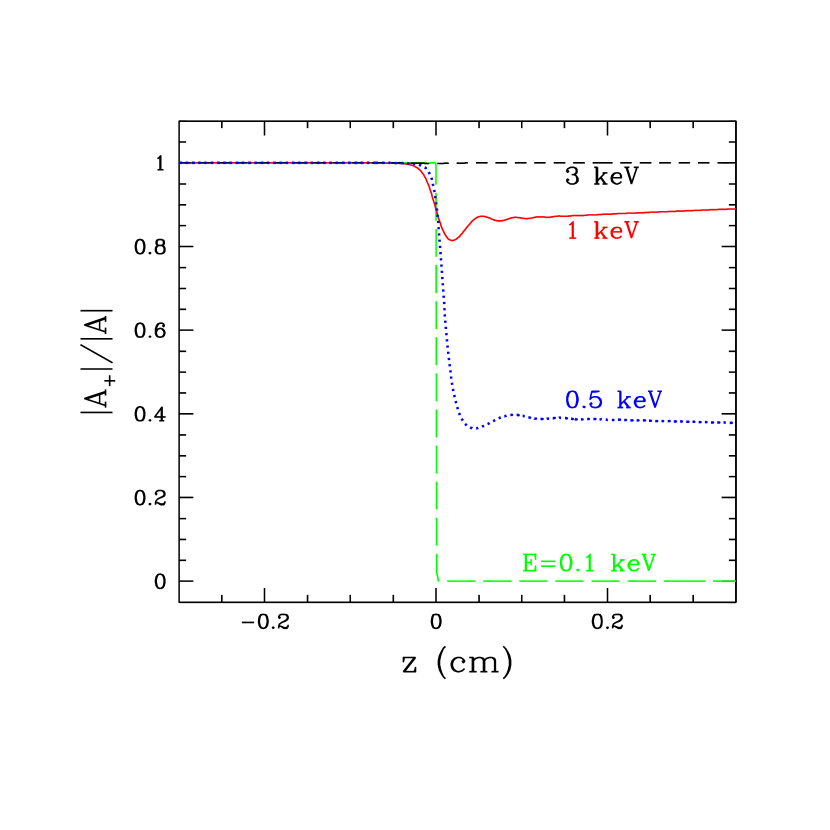
Figure 8: Evolution of the ratio $|A_{+}|/|A|$ for the cases depicted in Fig. 7. Here $|A_{\pm}|$ is the amplitude of the plus and minus-modes and $|A|=\sqrt{|A_{+}|^{2}+|A_{-}|^{2}}$.

The results of Fig. 7 are obtained using eq. (62). We can obtain the same results by integrating eq. (30) and calculating the Stokes parameters from eq. (43); this requires many more integration steps than using eq. (62) directly to achieve the same numerical accuracy. Since the photon modes are well-defined away from the vacuum resonance, we can calculate the mode amplitudes $A_{+}$ and $A_{-}$ from $A_{x}$ and $A_{y}$ [from integration of eq. (30)] using eq. (68). Figure 8 shows the evolution of the ratio $|A_{+}|/|A|$, where $|A|=(|A_{+}|^{2}+|A_{-}|^{2})^{1/2}$. Using eq. (42), we find that $P_{\rm jump}=1-3.2\times 10^{-7},~{}0.84,~{}0.27,~{}6.5\times 10^{-7}$ for $E=0.1,~{}0.5,~{}1,~{}3$ keV, respectively. Starting with $|A_{+}|/|A|=1$ before resonance, this implies $|A_{+}|/|A|=(1-P_{\rm jump})^{1/2}=5.7\times 10^{-4},~{}0.40,~{}0.85,~{}1$ after the resonance, in agreement with the numerical results shown in Fig. 8. Note that except for the $E=0.1$ keV case, the three other cases all lie in the large Faraday depolarization regime (see Figs. 4, 5), and the agreement between Fig. 8 and eq. (42) is not surprising.

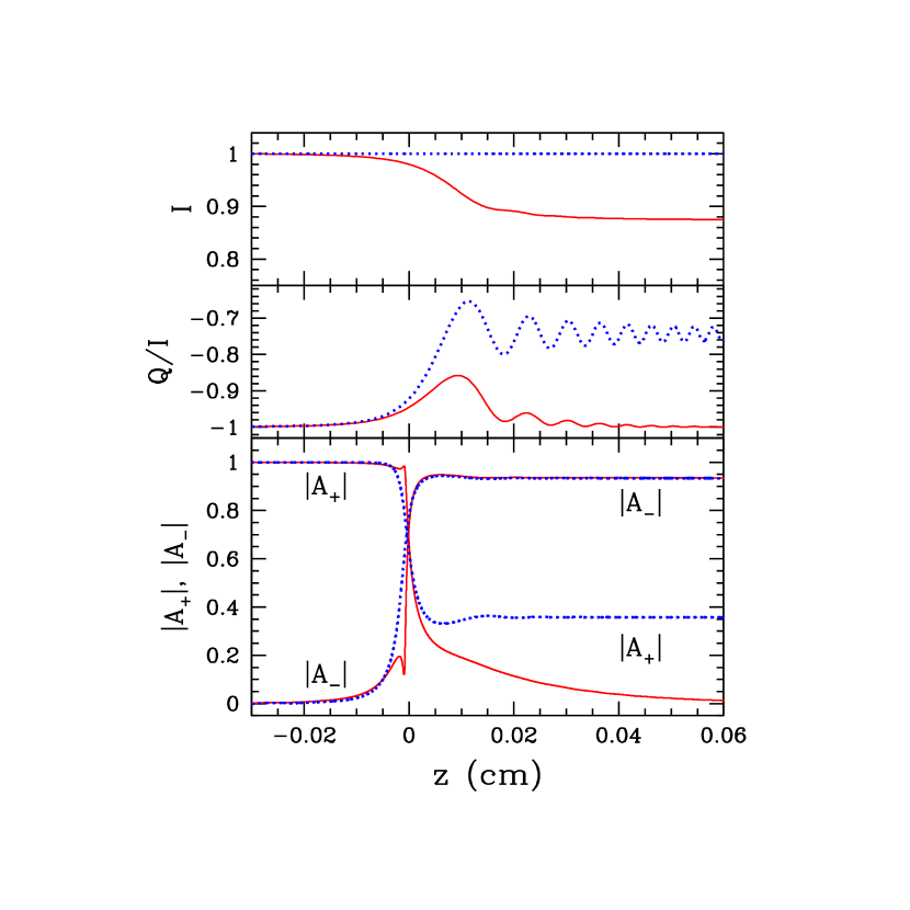
Figure 9: Evolution of Stokes parameters $I$, $Q$ and mode amplitudes $|A_{+}|,~{}|A_{-}|$ across vacuum resonance, for $E=1.7$ keV, $B_{14}=5$, $\theta_{B}=45^{\circ}$, and $H_{\rho}=5$ cm. At $z=-0.03$ cm, the radiation is in the plus-mode, with $A_{+}=1$. The solid lines show the results including realistic damping terms in the dielectric tensor, and the dotted lines show the results when the damping terms are turned off. Note that for this case, $\beta=1.066\,i$ at $\rho=\rho_{V}$, so that the mode amplitudes are well defined only away from the the resonance ($A_{+}$ and $A_{-}$ are calculated assuming that $\theta_{m}$ is real and the two modes are completely orthogonal).

Figure 9 shows another example of the evolution of polarized radiation, with $E=1.7$ keV, $B_{14}=5$, $\theta_{B}=45^{\circ}$ and $H_{\rho}=5$ cm. For this case, $\beta=1.066\,i$ at $\rho=\rho_{V}$, thus the two modes nearly collapse at the vacuum resonance. Nevertheless, we find that eq. (42) provides an accurate description for the evolution across the resonance: after the resonance, $|A_{-}|=P_{\rm jump}^{1/2}=0.93$ and decays slowly, while the plus-mode damps quickly because of the large opacity.

We note the distance over which resonant evolution occurs is much smaller than the the photon mean free path (see Figs. 7-9). We can estimate the width of the resonance as follows. From eq. (38) we have

$$\beta={u_{e}^{1/2}(1-u_{i})\sin^{2}\theta_{B}\over 2\cos\theta_{B}}\,\left(1-{\rho_{V}/\rho}\right).$$ (73)

At the resonance $\beta=0$. If we define the edge of the resonance region using the consition $|\beta|=\beta_{ed}\mathrel{\raise 1.29167pt\hbox{$>$}\mkern-14.0mu\lower 2.58334pt\hbox{$\sim$}}$ a few, we find the half-width of the resonance to be given by (LH02)

$$(\Delta z)_{V}={2\beta_{ed}H_{\rho}\cos\theta_{B}\over u_{e}^{1/2}|1-u_{i}|\sin^{2}\theta_{B}}$$

$$~{}\simeq 1.73\times 10^{-3}\beta_{ed}|1-u_{i}|^{-1}{\cos\theta_{B}\over\sin^{2}\theta_{B}}\left({E_{1}\over B_{14}}\right)H_{\rho}.$$ (74)

On the other hand, the imaginary parts of the indices of refraction of the two modes are given by

$${\rm Im}(n_{+}^{2})\simeq\gamma_{e}v_{e}\sin^{2}\theta_{B}\cos^{2}\theta_{m},$$ (75)

$${\rm Im}(n_{-}^{2})\simeq\gamma_{e}v_{e}\sin^{2}\theta_{B}\sin^{2}\theta_{m},$$ (76)

[valid for $u_{e}\gg 1$ and $u_{i}\ll 1$; cf. eq. (25)]. The mean free path $l$ is given by $l^{-1}=(\omega/c){\rm Im}(n^{2})$, and thus $l\geq c/(\omega\gamma_{e}v_{e})$ (the right-hand side being the mean free path at $B=0$). When collisional damping dominates, $\gamma_{e}\simeq\gamma_{ei}\gg\gamma_{re}$ [see eqs. (10)-(11)], we have

$$l\geq 0.26\,{AT_{6}^{1/2}E_{1}^{3}\over Z^{2}\rho_{1}^{2}(1-e^{-E/kT})g_{\alpha}^{\rm ff}}~{}{\rm cm}.$$ (77)

When scattering dominates, $l\geq 2.5\rho_{1}^{-1}$ cm. Thus the relation $l\gg(\Delta z)_{V}$ is almost always satisfied.

6 Transfer Equations for Stokes Parameters

Including the source term, the transfer equation reads [cf. eq. (62)]

$${d\over ds}{\mbox{\boldmath${\cal I}$}}={\hat{\bf k}}\cdot\nabla{\mbox{\boldmath${\cal I}$}}=-{\mbox{\boldmath${\cal M}$}}\cdot{\mbox{\boldmath${\cal I}$}}+{\mbox{\boldmath${\cal S}$}}_{\rm em}+{\mbox{\boldmath${\cal S}$}}_{\rm sc},$$ (78)

where we have used $ds$ (instead of $dz$) to specify the derivative along the ray. We derive the source functions ${\mbox{\boldmath${\cal S}$}}_{\rm em}$ and ${\mbox{\boldmath${\cal S}$}}_{\rm sc}$ below.

6.1 Source Function: Emission

The emissivity ${\mbox{\boldmath${\cal S}$}}_{\rm em}$ can be derived by considering the radiation field in thermodynamic equilibrium with matter, for which ${\mbox{\boldmath${\cal I}$}}=(B_{\nu}/2,B_{\nu}/2,0,0)^{+}$. Note that under this situation, ${\mbox{\boldmath${\cal S}$}}_{\rm sc}$ should completely cancel out the scattering contribution to ${\mbox{\boldmath${\cal M}$}}\cdot{\mbox{\boldmath${\cal I}$}}$ (see §6.2.2). Thus

$${\mbox{\boldmath${\cal S}$}}_{\rm em}={k_{0}B_{\nu}\over 2}\,\bigl{(}\sigma_{11i},\sigma_{22i},0,-2\sigma_{12r}\bigr{)}^{+}_{\rm em}.$$ (79)

This is equivalent to adding to the RHS of eq. (47) a source term

$$-k_{0}B_{\nu}\,\bigl{(}T_{0},T_{1},T_{2},T_{3}\bigr{)}^{+}_{\rm em}.$$ (80)

This is also the same as adding to the RHS of eq. (45) a term

$${1\over 4}k_{0}B_{\nu}\left(T_{\alpha\beta}+T_{\alpha\beta}^{+}\right)_{\rm em}.$$ (81)

The subscript “em” in eqs. (79)-(81) implies that the terms proportional to $\gamma_{re}=\gamma_{ri}$ should be excluded in evaluating these equations, since these terms are related to scattering contributions (§6.2.2). Equations (31)-(33) yield

$$\sigma_{11i}=\varepsilon_{i}\cos^{2}\theta_{B}+\eta_{i}\sin^{2}\theta_{B},$$ (82)

$$\sigma_{22i}=\varepsilon_{i},$$ (83)

$$\sigma_{12r}=-g_{i}\cos\theta_{B}.$$ (84)

From eqs. (7) and (8), we find

$$\hskip-14.22636pt\varepsilon_{i}\pm g_{i}={\rm Im}(\varepsilon\pm g)=$$

$$\Lambda_{\pm}\left[v_{e}\gamma_{ei}^{\pm}+(1\mp u_{i}^{1/2})^{2}v_{e}\gamma_{re}+(1\pm u_{e}^{1/2})^{2}v_{i}\gamma_{ri}\right],$$ (85)

$$\hskip-14.22636pt\eta_{i}={\rm Im}(\eta)=v_{e}\gamma_{ei}+v_{e}\gamma_{e}+v_{i}\gamma_{i},$$ (86)

where

$$\Lambda_{\pm}=\left[(1\pm u_{e}^{1/2})^{2}(1\mp u_{i}^{1/2})^{2}+\gamma_{\pm}^{2}\right]^{-1}$$ (87)

and

$$\gamma_{\pm}=\gamma_{ei}^{\pm}+(1\pm u_{e}^{1/2})\gamma_{ri}+(1\mp u_{i}^{1/2})\gamma_{re}.$$ (88)

Thus eq. (79) becomes

$$\hskip-8.5359pt{\mbox{\boldmath${\cal S}$}}_{\rm em}={k_{0}v_{e}B_{\nu}\over 4}\!\left[\begin{array}[]{c}{\cos^{2}\!\theta_{B}}\left(\Lambda_{+}\gamma_{ei}^{+}+\Lambda_{-}\gamma_{ei}^{-}\right)+2\gamma_{ei}\sin^{2}\!\theta_{B}\\ \Lambda_{+}\gamma_{ei}^{+}+\Lambda_{-}\gamma_{ei}^{-}\\ 0\\ 2\left(\Lambda_{+}\gamma_{ei}^{+}-\Lambda_{-}\gamma_{ei}^{-}\right)\cos\theta_{B}\end{array}\right].$$ (89)

Note that the terms in eq. (89) can be easily related to the free-free opacity: in magnetic fields, a photon of a certain polarization has an absorption opacity given by

$$\kappa^{\rm ff}=\kappa_{+}|e_{+}|^{2}+\kappa_{-}|e_{-}|^{2}+\kappa_{0}|e_{0}|^{2},$$ (90)

where $e_{0}=e_{Z}$, $e_{\pm}=(e_{X}\pm ie_{Y})/\sqrt{2}$ are the spherical components (with ${\bf B}$ along the $Z$-axis) of the photon’s unit polarization vector ${\bf e}$, and

$$\kappa_{\pm}={k_{0}\over\rho}v_{e}\gamma_{ei}^{\pm}\Lambda_{\pm},\quad\kappa_{0}={k_{0}\over\rho}v_{e}\gamma_{ei}.$$ (91)

Equation (91) agrees with (and generalizes to include the $Z>1$ case) the result of Potekhin & Chabrier (2002).

6.2 Source Function: Scattering

We first derive the source function due to electron scattering. The contribution from ion scattering can be easily added (see below).

Consider an incident EM wave with electric field ${\bf E}^{\prime}({\bf r},t)={\bf E}^{\prime}e^{i{\bf k}^{\prime}\cdot{\bf r}-i\omega t}$, where ${\bf E}^{\prime}=E_{x}^{\prime}{\hat{\bf e}}_{x^{\prime}}+E_{y}^{\prime}{\hat{\bf e}}_{y^{\prime}}$. In the coordinate system $XYZ$ with ${\bf B}$ along the $Z$-axis, the direction of the wave vector ${\bf k}^{\prime}=k_{0}{\hat{\bf k}}^{\prime}$ is specified by the polar angles $\theta_{B}^{\prime}$ and $\phi_{B}^{\prime}$. We define the directions of the unit vectors ${\hat{\bf e}}_{x^{\prime}}$ and ${\hat{\bf e}}_{y^{\prime}}$ such that ${\hat{\bf e}}_{x^{\prime}}$ lies in the meridian plane and points in the direction of increasing $\theta_{B}^{\prime}$, and ${\hat{\bf e}}_{x^{\prime}}\times{\hat{\bf e}}_{y^{\prime}}={\hat{\bf k}}^{\prime}$. Similarly, the scattered wave is denoted by ${\bf E}({\bf r},t)={\bf E}\,e^{i{\bf k}\cdot{\bf r}-i\omega t}$, where ${\bf E}=E_{x}{\hat{\bf e}}_{x}+E_{y}{\hat{\bf e}}_{y}$, and the polar angles for ${\hat{\bf k}}$ are $\theta_{B}$ and $\phi_{B}$. We also define unit vectors

$${\hat{\bf e}}_{\pm}=({\hat{\bf e}}_{X}\pm i{\hat{\bf e}}_{Y})/\sqrt{2},\quad{\hat{\bf e}}_{0}={\hat{\bf e}}_{Z}.$$ (92)

We can write the incident wave as

$${\bf E}^{\prime}=\sum_{\alpha=0,\pm}E_{\alpha}^{\prime}{\hat{\bf e}}_{\alpha}^{\ast},\quad{\rm with}~{}~{}E_{\alpha}^{\prime}={\hat{\bf e}}_{\alpha}\cdot{\bf E}^{\prime}.$$ (93)

(Here and henceforth, $\sum_{\alpha}$ refers to sum over $\alpha=0,\pm$). The scattered wave is given by the standard dipole formula ${\bf E}={\hat{\bf k}}\times({\hat{\bf k}}\times\ddot{\bf d})/(c^{2}r)$, with

$$\ddot{\bf d}=c^{2}r_{e}\sum_{\alpha}(1+\alpha u_{e}^{1/2})^{-1}E_{\alpha}^{\prime}{\hat{\bf e}}_{\alpha}^{\ast},$$ (94)

where $r_{e}=e^{2}/(m_{e}c^{2})$. Thus the Jones matrix relating ${\bf E}^{\prime}$ and ${\bf E}$ is given by

$$\left(\begin{array}[]{c}E_{x}\\ E_{y}\end{array}\right)=-{r_{e}\over r}\left[\begin{array}[]{cc}a&b\\ c&d\end{array}\right]\left(\begin{array}[]{c}E_{x}^{\prime}\\ E_{y}^{\prime}\end{array}\right),$$ (95)

where

$$a=\sum_{\alpha}(1+\alpha u_{e}^{1/2})^{-1}({\hat{\bf e}}_{x}\cdot{\hat{\bf e}}_{\alpha}^{\ast})({\hat{\bf e}}_{\alpha}\cdot{\hat{\bf e}}_{x^{\prime}}),$$ (96)

$$b=\sum_{\alpha}(1+\alpha u_{e}^{1/2})^{-1}({\hat{\bf e}}_{x}\cdot{\hat{\bf e}}_{\alpha}^{\ast})({\hat{\bf e}}_{\alpha}\cdot{\hat{\bf e}}_{y^{\prime}}),$$ (97)

$$c=\sum_{\alpha}(1+\alpha u_{e}^{1/2})^{-1}({\hat{\bf e}}_{y}\cdot{\hat{\bf e}}_{\alpha}^{\ast})({\hat{\bf e}}_{\alpha}\cdot{\hat{\bf e}}_{x^{\prime}}),$$ (98)

$$d=\sum_{\alpha}(1+\alpha u_{e}^{1/2})^{-1}({\hat{\bf e}}_{y}\cdot{\hat{\bf e}}_{\alpha}^{\ast})({\hat{\bf e}}_{\alpha}\cdot{\hat{\bf e}}_{y^{\prime}}).$$ (99)

Using ${\hat{\bf e}}_{x}=\cos\theta_{B}(\cos\phi_{B}{\hat{\bf e}}_{X}+\sin\phi_{B}{\hat{\bf e}}_{Y})-\sin\theta_{B}{\hat{\bf e}}_{Z}$ and ${\hat{\bf e}}_{y}=-\sin\phi_{B}{\hat{\bf e}}_{X}+\cos\phi_{B}{\hat{\bf e}}_{Y}$ (and similarly for ${\hat{\bf e}}_{x^{\prime}}$ and ${\hat{\bf e}}_{y^{\prime}}$), we find

$$a=\cos\theta_{B}^{\prime}\cos\theta_{B}\,{C^{(e)}({\Delta\phi})}+\sin\theta_{B}^{\prime}\sin\theta_{B},$$ (100)

$$b=\cos\theta_{B}\,{S^{(e)}({\Delta\phi})},$$ (101)

$$c=-\cos\theta_{B}^{\prime}\,{S^{(e)}({\Delta\phi})},$$ (102)

$$d={C^{(e)}({\Delta\phi})},$$ (103)

where

$${C^{(e)}({\Delta\phi})}={1\over 2}\left({e^{i\Delta\phi}\over 1-u_{e}^{1/2}}+{e^{-i\Delta\phi}\over 1+u_{e}^{1/2}}\right),$$ (104)

$${S^{(e)}({\Delta\phi})}={1\over 2i}\left({e^{i\Delta\phi}\over 1-u_{e}^{1/2}}-{e^{-i\Delta\phi}\over 1+u_{e}^{1/2}}\right),$$ (105)

with $\Delta\phi\equiv\phi_{B}-\phi_{B}^{\prime}$. Using the definition of ${\cal I}$ [see eq. (61)], we can relate ${\mbox{\boldmath${\cal I}$}}({\bf k})$ for the scattered radiation to ${\mbox{\boldmath${\cal I}$}}^{\prime}={\mbox{\boldmath${\cal I}$}}({\bf k}^{\prime})$ for the incident radiation. Integrating over all possible incident directions ${\hat{\bf k}}^{\prime}$, we obtain the source function due to electron scattering:

$${\mbox{\boldmath${\cal S}$}}_{\rm sc}^{(e)}({\bf k})=n_{e}r_{e}^{2}\int\!\!d\Omega^{\prime}\,\,{\bf R}^{(e)}({\bf k}^{\prime}\rightarrow{\bf k})\cdot{\mbox{\boldmath${\cal I}$}}({\bf k}^{\prime}),$$ (106)

where $d\Omega^{\prime}=d^{2}{\hat{\bf k}}^{\prime}=d\cos\theta_{B}^{\prime}d\phi_{B}^{\prime}$, and the scattering phase matrix ${\bf R}^{(e)}$ is given by

$$\hskip-22.76228pt{\bf R}^{(e)}({\bf k}^{\prime}\rightarrow{\bf k})=$$

$$\hskip-17.07182pt\left[\begin{array}[]{cccc}|a|^{2}&|b|^{2}&(a^{\ast}b)_{r}&(a^{\ast}b)_{i}\\ |c|^{2}&|d|^{2}&(c^{\ast}d)_{r}&(c^{\ast}d)_{i}\\ 2(a^{\ast}c)_{r}&2(b^{\ast}d)_{r}&(a^{\ast}d+b^{\ast}c)_{r}&(a^{\ast}d-b^{\ast}c)_{i}\\ -2(a^{\ast}c)_{i}&-2(b^{\ast}d)_{i}&-(a^{\ast}d+b^{\ast}c)_{i}&(a^{\ast}d-b^{\ast}c)_{r}\end{array}\right]$$ (111)

In eq. (111), we have used the notation $(a^{\ast}b)_{r}={\rm Re}(a^{\ast}b)$ and $(a^{\ast}b)_{i}={\rm Im}(a^{\ast}b)$, etc.

The source function due to photon-ion scattering can be similarly written as

$${\mbox{\boldmath${\cal S}$}}_{\rm sc}^{(i)}({\bf k})=n_{i}r_{i}^{2}\int\!\!d\Omega^{\prime}\,\,{\bf R}^{(i)}({\bf k}^{\prime}\rightarrow{\bf k})\cdot{\mbox{\boldmath${\cal I}$}}({\bf k}^{\prime}),$$ (112)

where $n_{i}$ is the ion number density, $r_{i}=(Ze)^{2}/(Am_{p}c^{2})$, and ${\bf R}^{(i)}$ has the same form as eq. (111), except that in the expressions for $a,b,c,d$ [eqs. (100)-(103)] one should replace ${C^{(e)}({\Delta\phi})}$ and ${S^{(e)}({\Delta\phi})}$ by

$${C^{(i)}({\Delta\phi})}={1\over 2}\left({e^{i\Delta\phi}\over 1+u_{i}^{1/2}}+{e^{-i\Delta\phi}\over 1-u_{i}^{1/2}}\right),$$ (113)

$${S^{(i)}({\Delta\phi})}={1\over 2i}\left({e^{i\Delta\phi}\over 1+u_{i}^{1/2}}-{e^{-i\Delta\phi}\over 1-u_{i}^{1/2}}\right).$$ (114)

It is easy to check the source functions derived above reduce to the appropriate zero-field results (Chandrasekhar 1960) when $B\rightarrow 0$.

6.2.1 Special Case: Axisymmetry

When ${\cal I}$ is independent of $\phi_{B}$ [as is the case when ${\bf B}$ is perpendicular to the (local) stellar surface], the source function ${\mbox{\boldmath${\cal S}$}}_{\rm sc}^{(e)}$ reduces to

$${\mbox{\boldmath${\cal S}$}}_{\rm sc}^{(e)}({\bf k})=2\pi n_{e}r_{e}^{2}\int\!d\mu^{\prime}\,\,\bar{\bf R}^{(e)}({\bf k}^{\prime}\rightarrow{\bf k})\cdot{\mbox{\boldmath${\cal I}$}}({\bf k}^{\prime}),$$ (115)

where $\mu^{\prime}=\cos\theta_{B}^{\prime}$. The azimuthal average of ${\bf R}^{(e)}$ is given by

$$\bar{\bf R}^{(e)}({\bf k}^{\prime}\rightarrow{\bf k})=\left[\begin{array}[]{cccc}\langle|a|^{2}\rangle&\mu^{2}F_{e}&0&\mu^{\prime}\mu^{2}G\\ \mu^{\prime 2}F_{e}&F_{e}&0&\mu^{\prime}G_{e}\\ 0&0&0&0\\ 2\mu^{\prime 2}\!\mu G_{e}&2\mu G_{e}&0&2\mu^{\prime}\!\mu F_{e},\end{array}\right]$$ (116)

where $\mu=\cos\theta_{B}$ and

$$\langle|a|^{2}\rangle=(\mu^{\prime}\mu)^{2}F_{e}+(1-\mu^{\prime 2})(1-\mu^{2}).$$ (117)

The functions $F_{e}$ and $G_{e}$ in eqs. (116)-(117) are

$$\hskip-5.69046ptF_{e}=\bigl{\langle}|C^{(e)}(\Delta\phi)|^{2}\bigr{\rangle}=\bigl{\langle}|S^{(e)}(\Delta\phi)|^{2}\bigr{\rangle}={1+u_{e}\over 2(1-u_{e})^{2}},$$ (118)

$$\hskip-5.69046ptG_{e}=i\Bigl{\langle}C^{(e)}(\Delta\phi)\left[S^{(e)}(\Delta\phi)\right]^{\ast}\Bigr{\rangle}=-{u_{e}^{1/2}\over(1-u_{e})^{2}}.$$ (119)

The source function ${\mbox{\boldmath${\cal S}$}}_{\rm sc}^{(i)}$ due to photon-ion scattering is

$${\mbox{\boldmath${\cal S}$}}_{\rm sc}^{(i)}({\bf k})=2\pi n_{i}r_{i}^{2}\int\!d\mu^{\prime}\,\,\bar{\bf R}^{(i)}({\bf k}^{\prime}\rightarrow{\bf k})\cdot{\mbox{\boldmath${\cal I}$}}({\bf k}^{\prime}),$$ (120)

where $\bar{\bf R}^{(i)}$ has the same form as eq. (116), except that the functions $F_{e}$ and $G_{e}$ are replaced by

$$F_{i}={1+u_{i}\over 2(1-u_{i})^{2}},\qquad G_{i}={u_{i}^{1/2}\over(1-u_{i})^{2}}.$$ (121)

6.2.2 Special Case: Thermodynamic Equilibrium

When the radiation field is in complete thermodynamic equilibrium with matter, ${\mbox{\boldmath${\cal I}$}}=(B_{\nu}/2,B_{\nu}/2,0,0)^{+}$, and the source functions due to electron and ion scatterings become

$${\mbox{\boldmath${\cal S}$}}_{\rm sc}^{(e)}({\bf k})=n_{e}\sigma_{T}B_{\nu}\left[\begin{array}[]{c}\mu^{2}F_{e}+(1-\mu^{2})/2\\ F_{e}\\ 0\\ 2\mu G_{e}\end{array}\right],$$ (126)

$${\mbox{\boldmath${\cal S}$}}_{\rm sc}^{(i)}({\bf k})=n_{i}\sigma_{T}^{(i)}B_{\nu}\left[\begin{array}[]{c}\mu^{2}F_{i}+(1-\mu^{2})/2\\ F_{i}\\ 0\\ 2\mu G_{i}\end{array}\right],$$ (131)

where $\sigma_{T}=8\pi r_{e}^{2}/3$ and $\sigma_{T}^{(i)}=8\pi r_{i}^{2}/3$. On the other hand, the sink term due to scattering is

$$\left({\mbox{\boldmath${\cal M}$}}\cdot{\mbox{\boldmath${\cal I}$}}\right)_{\rm sc}={k_{0}B_{\nu}\over 2}\,\bigl{(}\sigma_{11i},\sigma_{22i},0,-2\sigma_{12r}\bigr{)}^{+}_{\rm sc},$$ (132)

where the subscript “sc” implies that one should keep only the terms proportional to $\gamma_{re}$ and $\gamma_{ri}$ in eqs. (85)-(86) (the terms proportional to $\gamma_{ei}$ are due to absorption). Neglecting the damping $\gamma_{\pm}^{2}$ in eq. (87), we find $\varepsilon_{i}=2(v_{e}\gamma_{re}F_{e}+v_{i}\gamma_{ri}F_{i})$, $g_{i}=2(v_{e}\gamma_{re}G_{e}+v_{i}\gamma_{ri}G_{i})$, and $\eta_{i}=v_{e}\gamma_{re}+v_{i}\gamma_{ri}$. Substituting these into eqs. (82)-(84) and using

$$v_{e}\gamma_{re}=n_{e}\sigma_{T}/k_{0},\qquad v_{i}\gamma_{ri}=n_{i}\sigma_{T}^{(i)}/k_{0},$$ (133)

we can easily show that ${\mbox{\boldmath${\cal S}$}}_{\rm sc}^{(e)}+{\mbox{\boldmath${\cal S}$}}_{\rm sc}^{(i)}-\left({\mbox{\boldmath${\cal M}$}}\cdot{\mbox{\boldmath${\cal I}$}}\right)_{\rm sc}=0$ is satisfied, as it should.

7 Conclusion

The main results of this paper can be summarized as follows.

1. We presented a physical discussion of the effect of vacuum polarization on radiative transfer in strong magnetic fields and thermal radiation from magnetars (§2). This substantiated and clarified our previous results (LH02 and HL03): vacuum polarization depletes the high-energy tail of the thermal spectrum and suppresses spectral lines.

2. We studied the mode properties and examined several issues associated with the resonance due to vacuum polarization in a magnetized electron-ion plasma (§3). We showed that for superstrong magnetic fields, mode collapse and the breakdown of Faraday depolarization occur near the vacuum resonance for a wide range of propagation directions. Therefore a rigorous treatment of radiative transfer in magnetar atmospheres must go beyond the modal description of the radiation.

3. We studied the propagation of polarized radiation in the inhomogeneous atmosphere of magnetars (§4 and §5). We found that even with mode collapse and breakdown of Faraday depolarization, the evolution of polarized X-rays across the vacuum resonance can be described by a jump probability from one mode into another.

4. We derived the general transfer equations for the photon intensity matrix (Stokes parameters) in the magnetized plasma-vacuum medium (§6). Explicit expressions for the source functions due to emission and scatterings were obtained. These transfer equations are useful for accurate calculations of radiation/polarization spectra from magnetars.

Figure 4: The critical angle $\theta_{B}=\theta_{\rm coll}$ for mode collapse at vacuum resonance as a function of photon energy. The four curves correspond to $B_{14}=0.1,~{}1,5,~{}10$. Note that for $E=E_{Bi}$ (the ion cyclotron energy), $\theta_{\rm coll}$ is very close to $90^{\circ}$. For $\theta_{\rm coll}<\theta_{B}<180^{\circ}-\theta_{\rm coll}$, the modes are highly nonorthogonal and the condition for Faraday depolarization breaks down (see also Fig. 5).

Figure 5: The critical photon energy $E=E_{\rm Far}(B,\theta_{B})$ for the breakdown of Faraday depolarization. For $E\gg E_{\rm Far}$ (the unshaded region), the condition for large Faraday depolarization is satisfied. Note that the boundary $E=E_{\rm far}(B,\theta_{B})$ also corresponds to $\theta_{B}=\theta_{\rm coll}(E,B)$ (see Fig. 4).

Figure 6: The critical photon energy for adiabatic mode conversion as a function of magnetic field strength. The unshaded region refers to the adiabatic regime in which the condition $E>E_{\rm ad}$ is satisfied [see eq. (2)]. The solid line is for $\theta_{B}=45^{\circ}$ and the dashed line for $\theta_{B}=15^{\circ}$, both assuming $H_{\rho}=5$ cm.

Figure 7: Evolution of Stokes parameters across the vacuum resonance. The parameters are $B_{14}=1$, $\theta_{B}=45^{\circ}$, and the density profile is $\rho=\rho_{V}\exp({-z/H_{\rho}})$ with $H_{\rho}=5$ cm. At $z=-0.3$ cm, the radiation is in the plus-mode, with $I=1$. The solid lines are for $E=1$ keV, the short-dashed lines for $E=3$ keV, the dotted lines for $E=0.5$ keV, and the long-dashed lines for $E=0.1$ keV.

References

- (1) Adler, S.L. 1971, Ann. Phys., 67, 599
- Bezchastnov et al. (1996) Bezchastnov, V.G., Pavlov, G.G., Shibanov, Yu.A., & Zavlin, V.E. 1996, in Gamma-Ray Bursts, AIP Conf. Proc. Ser. vol. 384, eds. C. Kouveliotou et al. (NY: AIP), p.907
- Budden (1961) Budden, K.G. 1961, Radio Waves in the Ionosphere (Cambridge: Cambridge Univ. Press)
- Bulik & Miller (1997) Bulik, T. & Miller, M.C. 1997, MNRAS, 288, 596
- Chandrasekhar (1960) Chandrasekhar, S. 1960, Radiative Transfer (New York: Dover)
- (6) Dolginov, A.Z., Gnedin, Yu.N., & Silant’ev, N.A. 1970, J. Quant. Spectrosc. Radiat. Transfer, 10, 707
- (7) Dolginov, A.Z., & Pavlov, G.G. 1974, Sov. Astron., 17, 485
- Ginzburg (1970) Ginzburg, V.L. 1970, Propagation of Electromagnetic Waves in Plasmas (2d ed.; Oxford: Pergamon Press)
- Gnedin & Pavlov (1974) Gnedin, Yu.N. & Pavlov, G.G. 1974, Sov. Phys. JETP, 38, 903
- Gnedin et al. (1978a) Gnedin, Yu.N., Pavlov, G.G., & Shibanov, Yu.A. 1978a, Sov. Astron. Lett., 4, 117
- Gnedin et al. (1978b) Gnedin, Yu.N., Pavlov, G.G., & Shibanov, Yu.A. 1978b, JETP Lett., 27, 305
- Haxton (1995) Haxton, W.C. 1995, ARAA, 33, 459
- Heisenberg & Euler (1936) Heisenberg, W. & Euler, H 1936, Z. Physik, 98, 714
- Heyl & Hernquist (1997) Heyl, J.S. & Hernquist, L. 1997, J. Phys. A, 30, 6485
- Heyl & Shaviv (2000) Heyl, J. & Shaviv, N. 2000, MNRAS, 311, 555
- Ho & Lai (2001) Ho, W.C.G. & Lai, D. 2001, MNRAS, 327, 1081
- Ho & Lai (2002) Ho, W.C.G. & Lai, D. 2003, MNRAS, 338, 233 (astro-ph/0201380)
- (18) Ho, W.C.G., Lai, D., Potekhin, A.Y., & Chabrier, G. 2003, Advance in Space Research, submitted (astro-ph/0212077)
- Hurley (2000) Hurley, K. 2000, in Gamma-Ray Bursts: Fifth Huntsville Symposium, AIP Conf. Proc. 526, eds. R.M. Kippen et al. (New York: AIP), p.515
- Israel et al. (2001) Israel, G., Mereghetti, S., & Stella, L. 2001, Mem. Soc. Astron. Italiana, 73, in press (astro-ph/0111093)
- Juett et al. (2002) Juett, A.M., Marshall, H.L., Chakrabarty, D., & Schulz, N.S. 2002, ApJ, 568, L31
- Kubo & Nagata (1983) Kubo, H. & Nagata, R. 1983, J. Opt. Soc. Am., 73, 1719
- Lai & Ho (2002) Lai, D. & Ho, W.C.G. 2002a, ApJ, 566, 373 (LH02)
- (24) Lai, D. & Ho, W.C.G. 2002b, unpublished note (astro-ph/0204187)
- (25) Landau, L. 1932, Phys. Z. Sowjetunion, 2, 46
- Mészáros (1992) Mészáros, P. 1992, High-Energy Radiation from Magnetized Neutron Stars (Chicago: University of Chicago Press)
- Mészáros & Ventura (1978) Mészáros, P. & Ventura, J. 1978, Phys. Rev. Lett., 41, 1544
- Mészáros & Ventura (1979) Mészáros, P. & Ventura, J. 1979, Phys. Rev. D, 19, 3565
- Özel (2001) Özel, F. 2001, ApJ, 563, 276
- (30) Patel, S.K., et al. 2001, ApJ, 563, L45
- Pavlov & Gnedin (1984) Pavlov, G.G. & Gnedin, Yu.N. 1984, Sov. Sci. Rev. E, 3, 197
- Pavlov & Shibanov (1979) Pavlov, G.G. & Shibanov, Yu.A. 1979, Sov. Phys. JETP, 49, 741
- Pavlov et al. (2002) Pavlov, G.G., Zavlin, V.E., & Sanwal, D. 2002, in Proc. 270 WE-Heraeus Seminar on Neutron Stars, Pulsars, and Supernova Remnants, eds. W. Becker et al. (MPE Rep. 278; Garching: MPI), p.263 (astro-ph/0206024)
- Pavlov et al. (1995) Pavlov, G.G., Shibanov, Yu.A., Zavlin, V.E., & Meyer, R.D. 1995, in Lives of the Neutron Stars, eds. Alpar, M.A., Kiziloglu, U., & van Paradijs, J. (Boston: Kluwer), p.71
- Potekhin & Chabrier (2002) Potekhin, A.Y. & Chabrier, G. 2002, ApJ, in press
- Schwinger (1951) Schwinger, J. 1951, Phys. Rev., 82, 664
- Soffel et al. (1983) Soffel, M., Ventura, J., Herold, H., Ruder, H., & Nagel, W. 1983, A&A, 126, 251
- Thompson (2001) Thompson, C. 2001, in Neutron Star-Black Hole Connection, eds. C. Kouveliotou et al. (Dordrecht: Kluwer), p.369
- Thompson & Duncan (1996) Thompson, C. & Duncan, R.C. 1996, ApJ, 473, 322
- Tiengo et al. (2002) Tiengo, A., Goehler, E., Staubert, R., & Mereghetti, S. 2002, A&A, 383, 182
- Tsai & Erber (1975) Tsai, W.Y. & Erber, T. 1975, Phys. Rev. D, 12, 1132
- (42) Unno, W. 1956, Pub. Astron. Soc. Japan, 8, 108
- Ventura et al. (1979) Ventura, J., Nagel, W., & Mészáros, P. 1979, ApJ, 233, L125
- Zavlin & Pavlov (2002) Zavlin, V.E. & Pavlov, G.G. 2002, in Proc. 270 WE-Heraeus Seminar on Neutron Stars, Pulsars, and Supernova Remnants, eds. W. Becker et al. (MPE Rep. 278; Garching: MPI), p.263 (astro-ph/0206025)
- (45) Zener, C. 1932, Proc. R. Soc. London, Ser. A 137, 696
- Zheleznyakov et al. (1983) Zheleznyakov, V.V., Kocharovskiĭ, V.V., & Kocharovskiĭ, Vl.V. 1983, Sov. Phys. Usp., 26, 877
- (47) Zheleznyakov, V.V., Suvorov, E.V., & Shaposhnikov, V.E. 1974, Sov. Astron., 18, 142