Predictions for Cosmological Infrared Surveys from Space with the Multiband Imaging Photometer for SIRTF (MIPS).

Abstract

We make predictions for the cosmological surveys to be conducted by the Multiband Imaging Photometer for SIRTF (MIPS) at 24, 70 and 160 microns, for the guaranteed time observations and the legacy programs, using the latest knowledge of the instrument. In addition to the detector noise and the cirrus confusion noise, we discuss in detail the derivation of the confusion noise due to extragalactic sources, that depends strongly on the shape of the source counts at a given wavelength and on the telescope and detector pixel sizes. We show that it is wise in general to compare the classical photometric criterion, used for decades, and the so called source density criterion to predict the confusion levels. We obtain, using the model of Lagache, Dole, & Puget (2002) limiting fluxes of 50 $\mu$Jy, 3.2 mJy and 36 mJy at 24, 70 and 160 microns respectively. After taking into account other known sources of noise that will limit the surveys sensitivities, we compute the redshift distributions of the detected sources at each wavelength, and show that they extend up to z $\sim$ 2.7 at 24 $\mu m$ and up to z $\sim$ 2.5 at 70 and 160 $\mu m$, leading to resolve at most 69, 54 and 24% of the Cosmic Infrared Background (CIB) at 24, 70 and 160 microns respectively. We estimate which galaxy populations will be used to derive the luminosity function evolution with redshift. We also give the redshift distributions of the unresolved sources in the FIR range, that dominates the fluctuations of the CIB, and a predicted power spectrum showing the feasibility of fluctuations (both due to Poissonian and clustered source distributions) measurements. The main conclusion is that MIPS (and SIRTF in general) cosmological surveys will greatly improve our understanding of galaxy evolution by giving data with unprecedented accuracy in the mid and far infrared range.

1 Introduction

ISO, the Infrared Space Observatory, performed deep surveys in the mid (MIR) and far (FIR) infrared range (Genzel & Cesarsky, 2000; Franceschini et al., 2001, for reviews) in order to study galaxy evolution and to constrain the global star formation rate. Together with other surveys performed from the ground (e.g. with SCUBA and MAMBO), our view about galaxy evolution in the infrared, submillimeter and millimeter range became more accurate.

With the information extracted from these cosmological surveys, and in particular from the source counts, the redshift distribution of the sources, the spectral energy distribution of the Cosmic Infrared Background (CIB), and the analysis of the CIB fluctuations, it is possible to build a coherent view of galaxy evolution and formation in the infrared and submillimeter range by developing models that fit all the available data. Many semi-empirical models exist Roche & Eales (1999); Tan et al. (1999); Devriendt & Guiderdoni (2000); Dole et al. (2000); Wang & Biermann (2000); Chary & Elbaz (2001); Franceschini et al. (2001); Malkan & Stecker (2001); Pearson (2001); Rowan-Robinson (2001a, b); Takeuchi et al. (2001); Xu et al. (2001); Wang (2002) and try to address questions about the evolution of infrared galaxies, inferring the global star formation rate. These models fit reasonably well the data. Recently, Lagache, Dole & Puget (2002) have developed a phenomenological model which satisfies all the present observational constraints, one of which being the fluctuations of the background, as a powerful tool to investigate future observations.

The availability of new space facilities in the coming years, such as the Space Infrared Telescope Facility (SIRTF) in early 2003, ASTRO-F, and later in the decade Planck and Herschel, and on the ground with the Atacama Large Millimeter Array (ALMA), opens new perspectives to study in detail the population of infrared galaxies beyond z=1. Which galaxy populations these facilities will be able to detect ? What fraction of the CIB will be resolved into sources ? Up to what redshift will it be possible to construct a luminosity function and detect any evolution ? What will be the observational limitations on the cosmological surveys ?

To answer most of these questions prior to any new data being taken, and to better plan the surveys that will fully use the capabilities of these new facilities, it is common to use the models to make predictions, according to today’s knowledge. The goal of this paper is to investigate the properties of the planned SIRTF surveys with the Multiband Imaging Photometer for SIRTF (e.g. confusion, sensitivity, redshift distributions), using the Lagache et al. (2002) model as well as the latest knowledge of the MIPS instrument. Detailed predictions for Herschel, Planck and ALMA are given in Lagache et al. (2002).

The structure of the paper is as follows. The MIPS instrument and the planned surveys are described in Sect. 2. We discuss the confusion noise due to the galactic cirrus in Sect. 3. In Sect. 4 we summarize the Lagache et al. (2002) model, and one of its applications in Sect. 5: the generation of multiwavelength maps. The general case of the confusion noise due to extragalactic sources is discussed in Sect. 6, and the confusion limits for MIPS are given in Sect. 7. The total sensitivity for the surveys is given in Sect. 8. We discuss the expected results about resolved sources in Sect. 9 and about the unresolved sources in Sect. 10.

2 The MIPS Instrument and the Planned Cosmological Surveys

2.1 MIPS

MIPS, the Multiband Imaging Photometer for SIRTF Rieke et al. (1984); Young et al. (1998); Heim et al. (1998), is one of the three SIRTF Werner (1995) focal plane instrument, the others being the Infrared Camera, IRAC Fazio et al. (1998), and the Infrared Spectrograph, IRS Houck & Van Cleve (1995). MIPS is composed of three large array detectors, sensitive at 24, 70, and 160 $\mu m$ respectively. The array sizes are 128², 32² and $2\times 20$ pixels respectively, and the detector material is Si:As BIB, Ge:Ga and stressed Ge:Ga respectively. Among the main key features of MIPS, there are 1) the large size of the arrays, 2) the technical achievements in the detectors, 3) the calibration strategy of the FIR arrays Engelbracht et al. (2000) with frequent stimulator flashes tracking the responsivity variations, and 4) the presence of a scan mirror allowing an efficient and redundant sky coverage of 5 arcminute wide stripes, simultaneously at all three wavelengths.

The beam profile characteristics play an important role in computing the confusion limits; they have been generated using the STinyTim software, which is an updated version for SIRTF of the TinyTim software for HST Krist (1993). Tab. 1 summarizes the main characteristics of the pixels and beam profiles for MIPS.

Table 1: Some MIPS Instrumental Characteristics: Pixel size, Beam Profile, Noise

	24 $\mu m$	70 $\mu m$	160 $\mu m$
pixel size (”)	2.55	9.84	16.0
FWHM (”)a	5.6	16.7	35.2
pixel solid angle (sr)b	$1.41\times 10^{-10}$	$2.30\times 10^{-9}$	$5.87\times 10^{-9}$
$\int f(\theta,\phi)d\theta d\phi$ (sr)c	$1.25\times 10^{-9}$	$9.98\times 10^{-9}$	$4.45\times 10^{-8}$
$\int f^{2}(\theta,\phi)d\theta d\phi$ (sr)d	$4.27\times 10^{-10}$	$3.45\times 10^{-9}$	$1.66\times 10^{-8}$
1$\sigma_{p}$ for 10s integratione	0.22 mJy	2.0 mJy	6.6 mJy

2.2 Cosmological Surveys with MIPS

The currently planned Cosmological Surveys with MIPS are mainly scheduled through two types of programs: the GTOs (Guaranteed Time Observers) and the Legacy Programs. Deep IRAC observations are also planned for all programs, but are not discussed in this paper. The characteristics of all the following surveys are summarized in Tab. 2.

The MIPS GTO program for Cosmological Surveys is composed of three surveys, named Shallow, Deep and Ultra-Deep respectively, whose characteristics are listed in Tab. 2. The MIPS GTO program also includes galaxy cluster observations, aimed at mapping lensed background galaxies. In addition, some IRAC and IRS GTO programs share the same targets or directly contribute to some of them.

Two of the six Legacy Programs are focussed on cosmological surveys: SWIRE (SIRTF Wide-area InfraRed Extragalactic Survey) and GOODS (Great Observatories Origins Deep Survey). Schematically, for MIPS observations, the SWIRE surveys have the same observational strategy as the GTO shallow survey, but will cover a larger sky area (65 Sq. Deg.), and the GOODS surveys are similar to the GTO ultra-deep survey but will observe a 0.04 Sq. Deg. field at 24 $\mu m$ with more depth.

Finally, an early survey in the SIRTF mission will be conducted with MIPS and IRAC to verify the observational strategies: the First Look Survey (FLS) of the extragalactic component. Given the similarities with other surveys, we won’t discuss this survey specifically.

Table 2: MIPS Cosmological Survey Key Features

Survey	MIPS Observation	Area	24 $\mu m$	70 $\mu m$	160 $\mu m$
	Modea	Sq. Deg.b	$t_{int}$ (s)c	$t_{int}$ (s)c	$t_{int}$ (s)c
Shallowd	Scan Medium (2 passes)	9	80s	80s	8s
Deepd	Scan Slow (12 passes)	2.45 (6 $\times$ 0.41)	1200s	1200s	120s
Ultra Deepd	Photometry	0.02	14700s	12500s	–
Clustersd	Photometry	0.2 (28 $\times$ 0.007)	3300s	400s	80s
SWIREe	Scan Medium (2 passes)	65 (7 fields)	80s	80s	8s
GOODSe	Photometry	0.04	36000s	–	–
FLSf	Scan Medium (2 passes)	5	80s	80s	8s
FLS veriff	Scan Medium (10 passes)	0.25	400s	400s	40s

2.3 Sensitivity

The noise in the MIPS instrument is the sum of the detector-related noise (e.g. read noise, linearity correction noise, instantaneous flat field noise), the cosmic rays, and the photon noise. The noise budget is dominated by the photon noise (Rieke, private communication). For simplicity, we will call the total noise photon noise $\sigma_{p}$, even if all the instrumental noise sources are taken into account. Tab. 1 gives the 1 $\sigma_{p}$ noise in scan map mode for a 10s integration (Scan Map mode or Photometry Mode). The upper part of Tab. 5 gives the 1 $\sigma_{p}$ noise for the different integrations planned for the surveys. Notice that noise caused by any systematic effect is not taken into account here. It has been shown however for ISOCAM that the latter noise source do not degrade the final sensitivity Miville-Deschênes et al. (2000).

3 Cirrus Confusion Noise

Previous works Helou & Beichman (1990); Gautier et al. (1992); Kiss et al. (2001) studied in detail the confusion noise due to Galactic cirrus $\sigma_{gc}$, and showed that in most cases it can be simply parametrized as follows:

$$\rm\sigma_{gc}=0.3{\times}(\lambda_{100})^{2.5}(D_{m})^{-2.5}{\langle B_{\lambda}\rangle}^{1.5}$$ (1)

where $\sigma_{gc}$ is in mJy, $\lambda_{100}$ is the wavelength ratio ${\lambda}\over{100\,{\mu}m}$, $D_{m}$ is the telescope diameter in m, and $\langle B_{\lambda}\rangle$ is the brightness in MJy/sr Helou & Beichman (1990). Kiss et al. (2001) report that this parameterization underestimates $\sigma_{gc}$ by a factor of 2. However, their estimate of $\sigma_{gc}$ includes a contribution from CIB fluctuations which is known to be significant Lagache & Puget (2000), and so we can use the parameterization when we are only concerned with the Galactic cirrus component

Using Fig. 1 of Boulanger (2000) for the spectrum of the diffuse ISM, we extrapolate the mean brightness at 100 $\mu m$ $\langle B_{100}\rangle$ of 0.5 MJy.sr^-1 (corresponding to an HI column density of $10^{20}cm^{-2}$, typical for cosmological surveys) at 24, 70 and 160 $\mu m$. We then derive the corresponding cirrus confusion noise $\sigma_{gc}$ from Eq. 1. The results are given in Tab.3. For most of the cosmological fields, where the cirrus brightness $\langle B_{100}\rangle$ is less than 1 MJy.sr^-1, the cirrus confusion noise is often negligible or is a minor contribution to the total noise. In this work, we will thus only consider the confusion due to extragalactic sources, letting the reader adding the cirrus confusion noise appropriate to its own purpose.

Table 3: Cirrus Confusion Noise

	24 $\mu m$	70 $\mu m$	160 $\mu m$
$\langle B_{\lambda}\rangle$ MJy.sr-1a	0.03	0.12	1.5
$\sigma_{gc}^{b}$	0.06 $\mu$Jy	7.6 $\mu$Jy	2.7 mJy

4 Model of Infrared Galaxy Evolution

In addition to the photon noise and cirrus confusion noise, the noise due to the extragalactic sources is certainly the dominant noise for the cosmological surveys. The Lagache, Dole & Puget (2002) model is used to describe this component.

This model fits, besides the CIB intensity, source counts, the redshift distribution and colors, and the additional observational constraint of the CIB fluctuations. It describes only the dust emission part of the galaxies in the 4 $\mu m$ to 1.5 mm wavelength range. It is a phenomenological model based on two galaxy populations: the IR emission of normal spirals where optical output dominates and a starburst population. Each population is characterized by an SED family and an evolving luminosity function, described by a small number of parameters. The predictions of this model thus cover well the observed wavelength range from 8 $\mu m$ to 3 mm. It does not include source clustering. The confusion is computed for the Poisson contribution, and the clustering might slightly change the confusion limits; this will be investigated in forthcoming papers Blaizot et al., in prep ; Sorel et al., in prep .

The model outputs as well as some programs are publicly available on our web pages.

5 Simulating the Multi-Wavelength IR Sky

One of the applications of the model of Lagache et al. (2002) to plan future observations, is the creation of simulated maps of the infrared and submillimeter sky. The main purposes of the simulations are: 1) to test the calibration and map making algorithms, 2) to test and validate the source extraction and photometry procedures, check the completeness, and 3) to test other algorithms, such as HIRES or band merging procedures, to improve source detections in the FIR range. Results of these simulations will be the subject of a forthcoming paper.

The maps, available for public use upon request, are sampled with 2” pixels and have sizes ranging from $1024^{2}$ to $4096^{2}$ (0.32 to 5 Sq. Deg.). The simulated maps contain three components: an extragalactic component (IR galaxies), a galactic foreground component (cirrus), and a zodiacal light component. The following is a brief description of each component.

The Lagache et al. (2002) model evolving luminosity functions are used to create the extragalactic component in simulated maps over a wide range of wavelengths relevant to today and future studies (mainly for ISO, SIRTF, ASTRO-F, Planck, Herschel, SCUBA, MAMBO, ALMA). For computational efficiency, we add in the maps sources only in the redshift range 0 to 5.

The galactic foreground component, the cirrus, is build as follows: the spatial structure is taken from an actual 100 $\mu m$ cirrus in the IRAS recalibrated maps of Schlegel et al. (1998), and the scale extrapolation to smaller scales uses the properties of the cirrus power spectrum from Gautier et al. (1992). We then use the cirrus spectrum of Boulanger et al. (2000) to compute this component at other wavelengths.

The zodiacal light component is a constant value in our maps, taken from Tab.4 of Kelsall et al. (1998) for high ecliptic and galactic latitude fields.

6 Deriving the Confusion Noise due to Extragalactic Sources

Numerous authors Condon (1974); Hacking et al. (1987); Hacking & Soifer (1991); Franceschini et al. (1989, 1991); Vaisanen et al. (2001) have described the effect of the fluctuations due to the presence of point sources in a beam. For technological reasons limiting the telescope diameter compared to the wavelength, these fluctuations play an important (if not dominant) role in the measurements noise budget in the mid- and far-infrared, submillimeter and centimeter range for extragalactic surveys.

Through the rest of the paper, we will use the term confusion limit for confusion limit due to extragalactic sources. There are two different criteria to derive the confusion noise. The widely-used photometric criterion (Sect. 6.3) is derived from the fluctuations of the signal due to the sources below the detection threshold $S_{lim}$ in the beam; it was well adapted for the first generations of space IR telescopes (IRAS, COBE, ISO). The source density criterion (Sect. 6.4) is derived from a completeness criterion and evaluates the density of the sources detected above the detection threshold $S_{lim}$, such that only a small fraction of sources is missed because they cannot be separated from their nearest neighbor.

We will show that with SIRTF (or other planned telescopes), we need in general (regardless of the model used) to compare the confusion noise given by the two criteria, in order not to artificially underestimate the derived confusion noise. In the frame of the Lagache et al. (2002) model, we’ll give our estimates for the confusion.

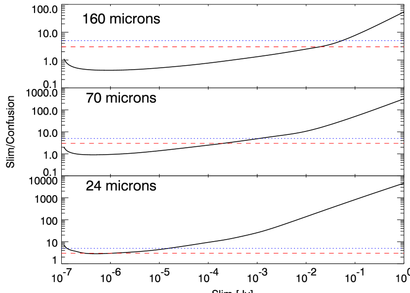
Figure 1: Signal to confusion noise ratio as a function of $S_{lim}$ at 24, 70 and 160 $\mu m$ (solid line). $S_{lim}/\sigma_{c}=3$ (dash) and $S_{lim}/\sigma_{c}=5$ (dot) are also plotted. At 24 $\mu m$, $S_{lim}/\sigma_{c}$ is always greater than 3; using the photometric criterion for deriving the confusion noise thus leads to a severe underestimation.

6.1 Confusion Noise: General Case

At a given frequency $\nu$ (hereafter the subscript $\nu$ will be omitted), let $f(\theta,\phi)$ be the two-dimensional beam profile (peak normalized to unity); let $S$ be the source flux density (hereafter flux) in Jy; let $dN/dS$ be the differential source counts in $Jy^{-1}sr^{-1}$.
The amplitude of the response $x$ due to a source of flux S at location ${\theta,\phi}$ within the beam is

$$x=Sf(\theta,\phi)$$ (2)

The mean number of responses, $R(x)$ with amplitudes between $x$ and $x+dx$, from sources present in the beam element $d\Omega$ at position $(\theta,\phi)$ (where $d\Omega=2\pi\theta d\theta d\phi$):

$$R(x)dx=\int_{\Omega}\frac{dN}{dS}dSd\Omega$$ (3)

The total variance $\sigma^{2}_{c}$ of a measurement within the beam due to extragalactic sources of fluxes less than $S_{lim}$ is given by:

$$\sigma_{c}^{2}=\int_{0}^{x_{lim}}x^{2}R(x)dx$$ (4)

where $x_{lim}=S_{lim}\times f(\theta,\phi)$ is the cutoff response at high flux. This can be rewritten as:

$$\sigma_{c}^{2}=\int f^{2}(\theta,\phi)d\theta d\phi\int_{0}^{S_{lim}}S^{2}\frac{dN}{dS}dS$$ (5)

We call $\sigma_{c}$ the confusion noise, and $S_{lim}$ the confusion limit. There are different ways of deriving $S_{lim}$, and they will be investigated in Sect. 6.3 and 6.4. Note that using Eq. 5 to determine the confusion limit is an approximation. A first refinement would be to use the limiting deflection $x_{lim}$ rather than $S_{lim}$, as explained by e.g. Condon (1974), and then introducing the effective beam. For MIPS, this changes the confusion level by less than 10%. Nevertheless, this refinement is not enough since it does not take into account other important parameters, related to the observational strategy and the analysis scheme, like the sky sampling, the pixelization (or PSF sampling), and the source extraction process, that also impact the confusion limit. Only complete realistic simulations would allow to predict accurately the confusion level; this next step will be addressed in a forthcoming paper using our simulations (Sect. 5). The method presented here aims at providing a theoretical prediction, which can be considered as a lower limit.

6.2 Beam Profiles

Before we obtain measurements of the telescope PSF (Point Spread Function) in flight, we need to use models of the beam profiles for the predictions of the confusion noise. A popular approximation is to use a Gaussian profile with the same FWHM than the expected PSF, although for SIRTF an Airy function should be more appropriate. The Gaussian profile is useful for analytical derivations of the confusion level as a function of the beam size Vaisanen et al. (2001). We want here to address the question of accuracy using the Gaussian approximation, the Airy approximation, or the modeled profile.

We compare the integral of the Gaussian profile (as written in Eq. 5) with the simulated profile obtained by STinyTim (Sect. 2.1): this leads to a small error in the first integral in Eq. 5 at the order of 2 to 10% depending on the MIPS wavelength; the difference is larger on the integral of the profile, about 30%. The Gaussian profile is thus a good approximation for computing analytically the confusion noise, but not for source extraction simulations.

Using an Airy profile gives better results for the profile integral, with a difference of less than 20%; the difference on the profile integrated according to Eq. 5 is worse, at the order of 10 to 35%. The Airy profile is thus better suited for source extraction simulations than for confusion noise estimates.

The use of the simulated STinyTim profiles (see Tab. 1) is at present our best approximation of the flight profiles. Indeed, Lagache & Dole (2001) have shown in the case of ISOPHOT that the theoretical profile is in good agreement with the actual profile.

6.3 The Photometric Criterion for Confusion Noise

The photometric criterion is defined by choosing the signal to noise ratio $q$ between the faintest source of flux $S_{lim}$, and the RMS noise $\sigma_{c}$ due to fluctuations from beam to beam (due to sources fainter than $S_{lim}$), as described in Eq. 6:

$$q=\frac{S_{lim}}{\sigma_{c\,phot}(S_{lim})}$$ (6)

$S_{lim}$, and thus $\sigma_{c}$, is found by solving Eq. 6 through an iterative procedure. $q$ is usually chosen with values between 3 to 5, depending on the objectives followed. Notice that $\sigma_{c\,phot}$ increases with $q$, as given in the upper part of Tab. 4. As a guideline, if one assumes a power law for the shape of the differential source counts ($\frac{dN}{dS}\propto S^{\alpha}$, with $\mid\alpha\,|<3$), then $\sigma_{c\,phot}$ varies with $q$ like $\sigma_{c\,phot}\propto q^{-\frac{3+\alpha}{1+\alpha}}$. This can be used in the Euclidean regime ($\mid\alpha\,|=2.5$). Note that $\alpha$ has the same meaning as $-\gamma$ in Condon (1974).

To illustrate the behavior of the implicit Eq. 6, Fig. 1 gives $S_{lim}/\sigma_{cphot}$ as a function of $S_{lim}$ given by Eq. 5, as well as the constant ratio $q=S_{lim}/\sigma_{cphot}$ for $q=$ 3 and 5. This plot illustrates that using $q=3$ at 24 $\mu m$ does not give a well defined solution, as the $S_{lim}=3\times\sigma_{c\,phot}$ line is almost tangent to the curve $\sigma_{c\,phot}(S_{lim})$; in this case, the signal to photometric confusion noise is always greater than three.

6.4 The Source Density Criterion for Confusion Noise

A second criterion for the confusion can be defined by setting the minimum completeness of the detection of sources above $S_{lim}$, which is driven by the fraction of sources lost in the detection process because the nearest neighbor with flux above $S_{lim}$ is too close to be separated. For a given source density $N$ (Poisson distribution) corresponding to sources with fluxes above $S_{lim}$, the probability P to have the nearest source of flux greater or equal to $S_{lim}$ located closer than the distance $\theta_{min}$ is:

$$P(<\theta_{min})=1-e^{-\pi N\theta_{min}^{2}}$$ (7)

Using $\theta_{FW}$, the Full Width at Half Maximum of the beam profile and $k$, we parameterize $\theta_{min}$ as:

$$\theta_{min}=k\times\theta_{FW}$$ (8)

Fixing a value of the probability $P$ gives a corresponding density of sources, $N_{SDC}$ (SDC stands for Source Density Criterion):

$$N_{SDC}=-\frac{log(1-P(<\theta_{min}))}{\pi k^{2}\theta_{FW}^{2}}$$ (9)

At a given wavelength, there is a one-to-one relationship between the source density and the flux, given by the source counts; thus $S_{SDC}$ is determined with $N_{SDC}$ with our source count model. We identify $S_{SDC}$ as $S_{lim}$, and can then compute the confusion noise using the source density criterion $\sigma_{SDC}$ using Eq. 5, as a function of P and k.

We define the source density criterion for deriving the confusion noise, by choosing a value of $P(<\theta_{min})$ and $k$, the latter can be determined e.g. by simulations. $S_{lim}$ is the limiting flux, such as there is a chosen probability $P(<\theta_{min})$ of having two sources of flux above $S_{lim}$ at a distance of less than $\theta_{min}=k\,\theta_{FW}$.

We made simulations of source extraction with DAOPHOT and checked that $k=0.8$ is an achievable value; this is also in agreement with the results from Rieke et al. (1995). We thus use $k=0.8$. We use $P=10$%, meaning that 10% of the sources are too close to another source to be extracted. The corresponding source density is, as explained in Tab. 1 of Lagache et al. (2002), $1/16.7\,\Omega$. The middle part of Tab. 4 gives $S_{lim\,sdc}$ using the Source Density Criterion, and the corresponding equivalent $q_{sdc}$ which is the ratio $S_{lim}/\sigma_{sdc}$.

One the one hand, the Photometric and Source Density criteria give almost identical results in the simple Euclidean case, if one takes $q=3$, $k=1$, and a maximum probability to miss a source too close to another one of 10%. In this classical case, confusion becomes important for a source density corresponding to one source per 30 independent instrumental beams. On the other hand, when the relevant LogN-LogS function departs strongly from Euclidean, the two criteria give very different results for these reasonable values of $q$, $k$, and $P$. Furthermore, for specific astrophysical problems, one might want to choose significantly different values of these parameters. In that case, the two criteria might not be equivalent. For instance at 70 $\mu m$, increasing P to 20%, 45% and 60% respectively (instead of the 10% we’re using), give a confusion limit identical to q=5, 4 and 3 respectively, even if in the last case 60% of the sources will be missed.

7 Confusion Limits for MIPS and Comparison with Other Works

7.1 Confusion Limits for MIPS

Comparing the photometric (Sect. 6.3) and the source density (Sect. 6.4) criteria for the confusion, we conclude that for MIPS, the source density criterion is always met before (i.e. at higher flux) the photometric criterion using $q\simeq 4$. At 160 $\mu m$, the two criteria become identical. Lagache et al. (2002) show that for all the IR/submm space telescopes of the coming decade, the break point between the two criteria is at around 200 $\mu m$.

SIRTF, together with its high sensitivity and its well sampled PSFs, will probe a regime in the source counts where the classical photometric criterion is no longer valid. The main reasons are 1) the steep shape of the source counts, and 2) the fact that a significant part of the CIB will be resolved into sources (Sect. 9.4). This leads to a high source density at faint detectable flux levels, that actually limits the ability to detect fainter sources. In this case, the limiting factor is not the fluctuations of the sources below the detection limit (photometric criterion) but the high source density above the detection limit (source density criterion).

For SIRTF, we thus use the source density criterion for deriving the confusion noise and limit.

For the previous generations of infrared telescopes (IRAS, ISO), it is interesting to compare the two criteria, and usually they converge to the same answer – a direct consequence of undersampling a large PSF that doesn’t allow to probe deeper the source counts. In this case, the photometric criterion is applicable and has been widely used.

The confusion noise and the confusion limit for MIPS are given in the lower part of Tab. 4.

Fig. 2 represents the integral source counts at 24, 70 and 160 $\mu m$ respectively. At these wavelengths, the confusion limits, given in Tab. 4, correspond to source densities of $6.9\times 10^{7}$, $7.8\times 10^{6}$, and $1.9\times 10^{6}$ per steradian at 24, 70 and 160 $\mu m$ respectively. This corresponds to 11.5, 12.8 and 12.0 beams per sources at 24, 70 and 160 $\mu m$ respectively. The derived values are slightly lower than the “generic” case discussed in Sect. 6.4 of 16.7 sources per beam, the difference coming from the use of a simulated beam profile rather than a Gaussian profile.

7.2 ISO at 170 $\mu m$

The data of the 4 Sq. Deg. FIRBACK survey Dole et al. (2001) performed with ISO at 170 $\mu m$ allowed to directly measure the sky confusion level. This provides a rare opportunity to test the model.

The confusion level was measured at 170 $\mu m$ at 1$\sigma_{c}=45$ mJy, and the 4$\sigma_{c}$ limit (180 mJy) corresponds to 52 beams per source Dole et al. (2001).

Using our model with the actual PSF Lagache & Dole (2001) and the photometric criterion (valid in this case), we obtain 1$\sigma_{c}=40$ mJy, and for $q=4$, $S_{lim}=158$ mJy; this flux limit corresponds to 40 beams per source.

The good agreement comforts the quality of the model for estimating the confusion level from modeled source counts.

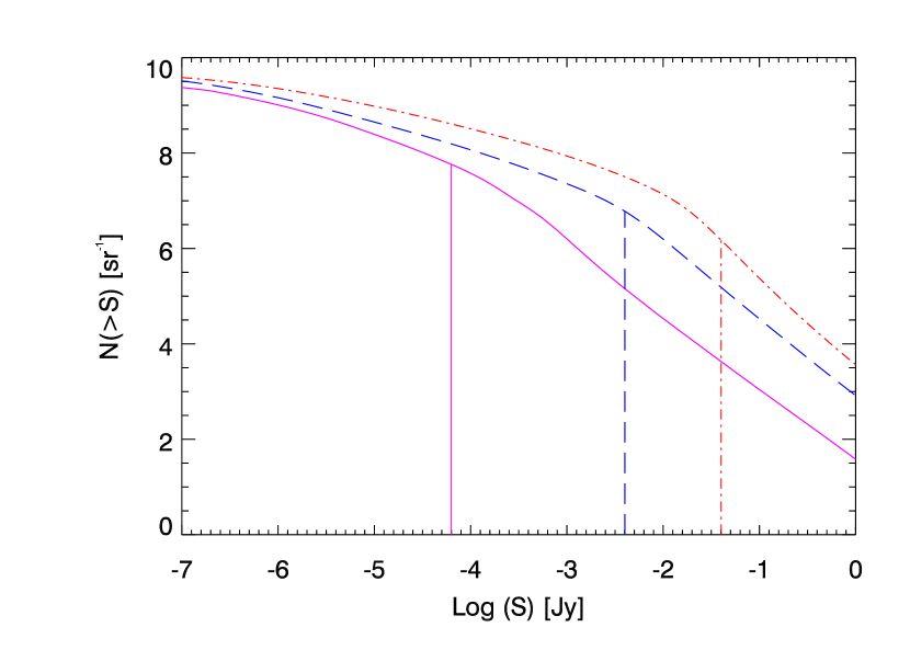
Figure 2: Integral Source Counts from our model at 24 (line), 70 (dash) and 160 $\mu m$ (dot-dash), and Confusion Limits $S_{lim}$ from Tab. 4.

Table 4: Confusion Limits with different Criteria, and Final Confusion Limits

	24 $\mu m$	70 $\mu m$	160 $\mu m$
$S_{lim}$ and $q$ using the Photometric Criteriona
$S_{lim}$, $q=3$	–	0.20 mJy	20 mJy
$S_{lim}$, $q=4$	7.1 $\mu$Jy	0.56 mJy	40 mJy
$S_{lim}$, $q=5$	15.8 $\mu$Jy	1.12 mJy	56 mJy
$S_{lim}$ and $q$ using the Source Density Criterionb
$S_{lim}$	50 $\mu$Jy	3.2 mJy	36 mJy
$q_{sdc}$	7.3	6.8	3.8
$S_{lim}$ and $q$ using the Best Estimatorc
$S_{lim}$	50 $\mu$Jy	3.2 mJy	36.0 mJy
$q$	7.3d	6.8d	3.8d,e

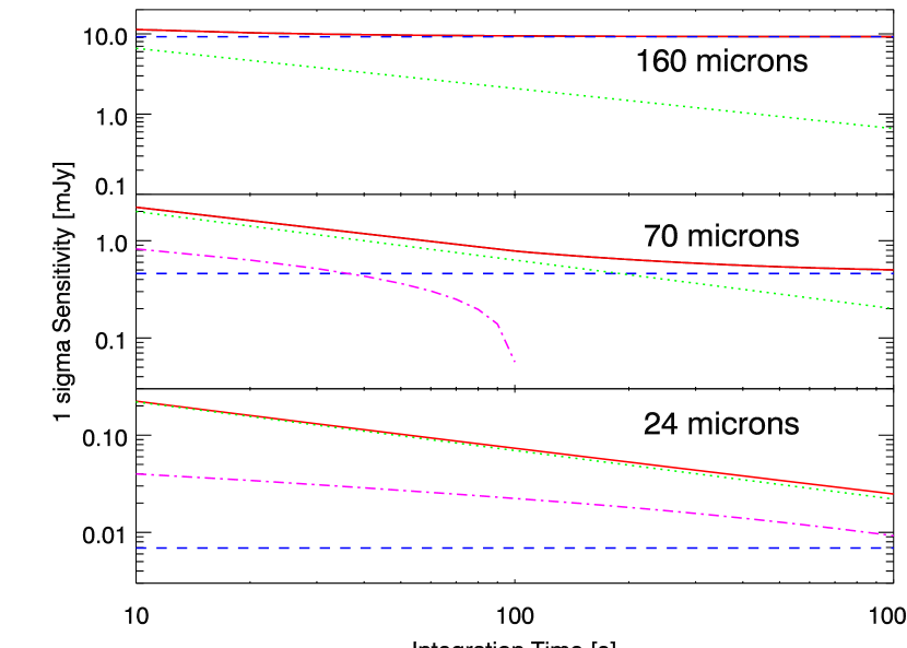
Figure 3: $1\sigma$ sensitivity of the scan maps as a function of integration time at 24, 70 and 160 $\mu m$. Solid Line: Total $1\sigma$ Sensitivity; Dash: Confusion level $\sigma_{c}$ ; Dot: photon noise; Dash-dot: additional confusion noise.

7.3 Comparison with Other Determinations

Xu et al. (2001) computed the confusion limit $S_{lim}$ with the photometric criterion using $q=3$ for MIPS and get 33 $\mu$Jy, 3.9 mJy and 57 mJy at 24, 70 and 160 $\mu m$ respectively. This corresponds respectively to 8, 17 and 31 beams per source. Our estimates are thus compatible at 70 $\mu m$, but slightly different at 24 and 160 $\mu m$. Their use of the photometric criterion at 24 $\mu m$ significantly underestimates the confusion level. At 160, their redshift distribution seems to overestimate (at the FIRBACK flux limits) the population peaking at z $\sim$ 1 Patris et al. (2002), which may suggest a difference in the $dN/dS$ distribution, that directly affects the predicted confusion levels.

Franceschini et al. (2002), based on the model of Franceschini et al. (2001), give preliminary $5\sigma_{c}$ confusion limits for MIPS at 24, 70 and 160 $\mu m$ and get 85 $\mu$Jy, 3.7 and 36 mJy respectively. This corresponds respectively to 19, 15 and 12 beams per source. The values for the far infrared are in good agreement with our predictions. However, a more refined comparison needs to be done when details of their computation will be published, especially in the mid infrared.

Other models exist Roche & Eales (1999); Tan et al. (1999); Devriendt & Guiderdoni (2000); Wang & Biermann (2000); Chary & Elbaz (2001); Pearson (2001); Rowan-Robinson (2001b); Takeuchi et al. (2001); Wang (2002), but do not specifically address the point of predicting the confusion limits for SIRTF. Malkan & Stecker (2001) and Rowan-Robinson (2001a) make predictions. The former use, as a photometric criterion, 1 source per beam. The latter uses 1 source per 40 beams, leading to $S_{lim}$ of 135 $\mu$Jy, 4.7 mJy and 59 mJy at 24, 70 and 160 $\mu m$ respectively.

7.4 The 8 $\mu m$ Case

Our model reaches its limit around 8 $\mu m$ because our SEDs are not designed for wavelengths shorter than $4\mu m$. However, it fits all observables at wavelengths longer than 7 $\mu$m. We can thus predict the confusion level. As for the 24 $\mu m$, the confusion level will be low, and will not limit the extragalactic surveys.

At 8 $\mu m$, the photometric criterion does not provide a meaningful confusion limit because the $S_{lim}/\sigma_{c}$ ratio is always greater than 10. We obtain, using the source density criterion, $S_{lim}=0.45\,\mu$Jy and $\sigma_{c}=0.05\,\mu$Jy, leading to $q=9.72$.

The values from Vaisanen et al. (2001) are $S_{lim}=3-4\,\mu$Jy, $\sigma_{c}=0.40-0.51\,\mu$Jy and $q=10.0$. Our estimation of the confusion level for this IRAC band is lower by a factor of $\sim 7$. This discrepancy comes in fact from the source counts themselves: we underpredict the source density by a factor 7 to 8 in the range at 0.1 to 1 $\mu$Jy, even if both models reproduce the ISO counts. This is expected from a model which accounts properly for the dust emission but does not model the stellar emission of high redshift galaxies. When using the counts from Vaisanen et al. (2001), we agree with their published values. Vaisanen et al. (2001), in their Sect. 5.3, discuss the sensitivity of the predicted confusion levels to the shape of the source counts, and the constraints of the modeled source counts by the data. Their conclusion is that, although the 7 $\mu m$ ISOCAM source counts above 50 $\mu$Jy agree within uncertainties, the models below 1 $\mu$Jy are not much constrained. As a result, the predictions for the confusion level down to the IRAC sensitivity can be as different as a factor of 10. We confirm this analysis.

8 Sensitivity in the MIPS Final Maps

In this section we compute the sensitivity of the MIPS surveys as a function of the integration time. The total noise $\sigma_{tot}$ is Lagache et al. (2002):

$$\sigma_{tot}=\sqrt{\sigma_{p}^{2}+\sigma_{c}^{2}+\sigma_{add}^{2}}$$ (10)

where $\sigma_{p}$ is the photon noise (Sect. 2.3), $\sigma_{c}$ is the confusion noise (Sect. 7 & Tab. 4), and $\sigma_{add}$ is the additional confusion noise. This additional confusion noise is only present when the photon noise exceeds the confusion noise: in this case, $\sigma_{add}$ accounts for the confusion due to bright sources above the confusion limit but below the photon noise. $\sigma_{add}$ is computed, when $5\sigma_{p}>S_{lim}$:

$$\sigma_{add}^{2}=\int f^{2}(\theta,\phi)d\theta d\phi\int_{S_{lim}}^{5\sigma_{p}}S^{2}\frac{dN}{dS}dS$$ (11)

Fig. 3 shows $\sigma_{tot}$ and the relative contributions of $\sigma_{p}$, $\sigma_{c}$ and $\sigma_{add}$ as a function of the integration time. It appears that the 160 $\mu m$ data are confusion limited even with short integrations. At 70 $\mu m$, the confusion should dominate the noise for exposures longer than 100s, and $\sigma_{add}$ is a small component in the first 50s and is negligible after. At 24 $\mu m$ we do not expect the data to be confusion limited, and $\sigma_{add}$ is between 5 and 3 times smaller than the photon noise.

Table 5: Sensitivities of the planned Cosmological Surveys: 1 $\sigma_{p}$ (photon noise only), 1 $\sigma_{tot}$, and final sensitivity (see text).

	24 $\mu m$	70 $\mu m$	160 $\mu m$
1 $\sigma_{p}$ Sensitivity (does not include sky confusion)a
Shallow 1$\sigma_{p}$	78 $\mu$Jy	0.71 mJy	6.6 mJy
Deep 1$\sigma_{p}$	20 $\mu$Jy	0.18 mJy	1.9 mJy
Ultra Deep 1$\sigma_{p}$	6 $\mu$Jy	0.06 mJy	–
Clusters 1$\sigma_{p}$	12 $\mu$Jy	0.32 mJy	2.3 mJy
SWIRE 1$\sigma_{p}$	78 $\mu$Jy	0.71 mJy	6.6 mJy
GOODS 1$\sigma_{p}$	4 $\mu$Jy	–	–
1 $\sigma_{tot}$ Final Sensitivity of the Surveysb
Shallow 1 $\sigma_{tot}$	82 $\mu$Jy	0.87 mJy	11.3 mJy
Deep 1 $\sigma_{tot}$	23 $\mu$Jy	0.49 mJy	9.4 mJy
Ultra Deep 1 $\sigma_{tot}$	9 $\mu$Jy	0.46 mJy	–
Clusters 1 $\sigma_{tot}$	15 $\mu$Jy	0.55 mJy	9.5 mJy
SWIRE 1 $\sigma_{tot}$	82 $\mu$Jy	0.87 mJy	11.3 mJy
GOODS 1 $\sigma_{tot}$	8 $\mu$Jy	–	–
Final sensitivities of the Surveysc
Shallow	392 $\mu$Jy	4.7 mJy	48 mJy
Deep	112 $\mu$Jy	3.2 mJy	36 mJy
Ultra Deep	59 $\mu$Jy	3.1 mJy	–
Clustersd	79 $\mu$Jy	3.5 mJy	37 mJy
SWIRE	392 $\mu$Jy	4.7 mJy	48 mJy
GOODS	54 $\mu$Jy	–	–

The middle part of Tab. 5 gives the $1\sigma_{tot}$ sensitivity for the surveys, and includes the confusion, the instrumental and the additional confusion noise components. Notice that these $1\sigma_{tot}$ values are given as a guideline, knowing that taking $5\sigma_{tot}$ for the survey sensitivities is an approximation, since $S_{lim}$ does not equal $5\sigma_{c}$ in the general case, as discussed in Sect. 7.1.

The bottom part of Tab. 5 gives the fluxes that will limit the surveys. They are computed by using the approximation given by the quadratic sum $\sqrt{5\sigma_{p}^{2}+S_{lim}^{2}}$, which provides a smooth transition between the regime dominated by photon/detector noise (24 $\mu m$) and the regime dominated by confusion noise (160 $\mu m$). These values are taken to be the baseline for the further discussions. The final sensitivity for the 65 Sq. Deg. the SWIRE Legacy survey will be the same as the GTO Shallow survey. The deep GTO surveys will be almost 4 times more sensitive (photon noise) that the shallow ones, on about 2.5 Sq. Deg.; in the far infrared, the confusion will nevertheless limit the final sensitivity. For the GOODS Legacy program, with 10h integration per sky pixel at 24 $\mu m$ on 0.04 Sq. Deg., we expect a final sensitivity of 54 $\mu$Jy at 24 $\mu m$.

It is beyond the scope of this paper to investigate the properties of the galaxy cluster targets of the SIRTF GTO program and to make predictions, but in these fields, the confusion limits will significantly be reduced due to the gravitational lensing by a foreground rich cluster, which increases both the brightness and mean separation of the background galaxies. This effect has already been exploited successfully in the mid-infrared (e.g. ISO, Altieri et al., (1999)) and in the submillimeter (e.g., SCUBA Lens Survey, Smail et al., (2002)). The SIRTF GTO program will apply the same strategy in the mid- and far-IR. The lensed area of the proposed GTO program is expected to cover 90 Sq. arcmin (E. Egami, Private Communication).

Other effects, not included in this analysis, might slightly degrade the final sensitivity of the maps, especially on Ge:Ga detectors at 70 and 160 $\mu m$; these effects, well characterized on the ground, can probably be corrected with an accuracy of a few percent using data redundancy and a carefully designed pipeline Gordon et al. (in prep). The effects are: stimulator flash latents (the amplitude is less than $3\%$ and the exponential decay time constant is in the range 5-20 s), transients, responsivity changes (tracked with the stimulator flashes every 2 minutes), and cosmic ray hits related noise. The final sensitivity will be measured in the first weeks of operation, during the In Orbit Checkout and Science Verification phases.

Table 6: Number of Expected Sources in the MIPS Surveys, and Fraction of the CIB that will be resolved into sources (assuming that all sources are unresolved). Characteristics of the Surveys is given in Tab. 2.

	24 $\mu m$	70 $\mu m$	160 $\mu m$
Number of Expected Sources
Shallow	$2.0\times 10^{4}$	$1.3\times 10^{4}$	$2.8\times 10^{3}$
Deep	$2.5\times 10^{4}$	$5.8\times 10^{3}$	$1.4\times 10^{3}$
Ultra Deep	$3.7\times 10^{2}$	$49$	–
SWIRE	$1.5\times 10^{5}$	$1.0\times 10^{5}$	$2.2\times 10^{4}$
GOODS	$8.4\times 10^{2}$	–	–
Fraction of Resolved CIB
Shallow	35%	46%	18%
Deep	58%	54%	23%
Ultra Deep	68%	54%	–
SWIRE	35%	46%	18%
GOODS	69%	–	–

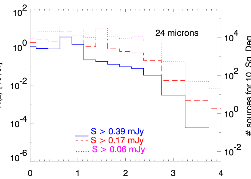
Figure 4: Redshift Distribution at 24 $\mu m$ with MIPS. Solid Line: Shallow Survey; Dash: Deep Survey; Dot: Ultra Deep Survey. The flux limits are listed in Tab. 5. Left axis gives the source density (number of sources for the particular bin sizes shown), right axis gives the number of sources in a 10. Sq. Deg. field.

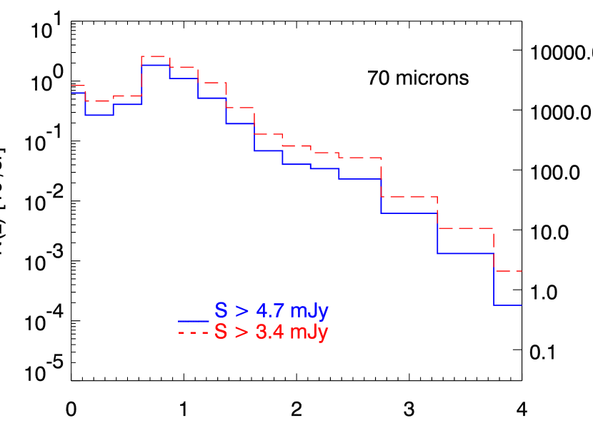
Figure 5: Redshift Distribution at 70 $\mu m$ with MIPS. Solid Line: Shallow Survey; Dash: Deep Survey; Dot: Ultra Deep Survey. The flux limits are listed in Tab. 5. Left axis gives the source density (number of sources for the particular bin sizes shown), right axis gives the number of sources in a 10. Sq. Deg. field.

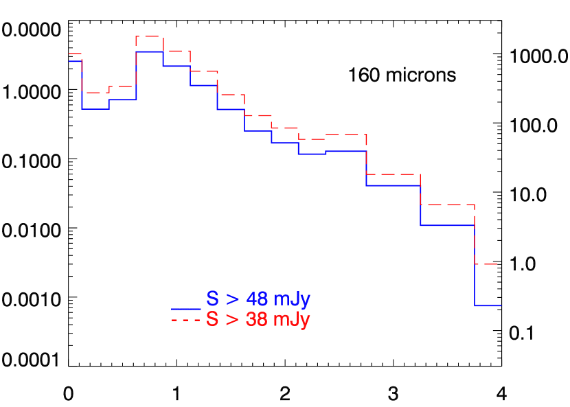
Figure 6: Redshift Distribution at 160 $\mu m$ with MIPS. Solid Line: Shallow Survey; Dash: Deep Survey. The flux limits are listed in Tab. 5. Left axis gives the source density (number of sources for the particular bin sizes shown), right axis gives the number of sources in a 10. Sq. Deg. field.

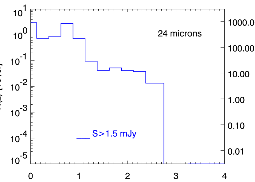
Figure 7: Redshift Distribution at 24 $\mu m$ with MIPS for sources brighter than 1.5 mJy and 0.75 mJy, allowing a spectroscopic follow-up with IRS. Left axis gives the source density (number of sources for the particular bin sizes shown), right axis gives the number of sources in a 10. Sq. Deg. field. In the proposed 9 Sq. Deg. shallow survey, we would expect 2100 and 7200 sources to the 1.5 and 0.75 mJy depth respectively.

Figure 8: Number of starburst galaxy per logarithmic luminosity bin ($\Delta\ln{L}/\ln{L}=0.1$) that can be detected at different redshifts (with a $\Delta$z/z=0.5). Top: 160 $\mu$m survey of 80 Sq. Deg. (surface covered by SWIRE and the GTO) limited by the confusion at 48 mJy. Middle: 70 $\mu$m survey of 80 Sq. Deg. limited by the confusion at 4.7 mJy. Bottom: 24 $\mu$m survey of 2.46 Sq. Deg. down to 112 $\mu$Jy (GTO Deep Survey). The horizontal dash line shows the 50 sources needed in a $\Delta$z/z=0.5 bin and $\Delta\ln{L}/\ln{L}=0.1$ bin for reconstructing the Luminosity Function (LF). From bottom left to upper right, redshift bins centered at z=0.01, 0.1, 0.5, 0.7, 1.0, 2.5.

9 Resolved Sources: Redshift Distributions, Luminosity Function, Resolution of the CIB

9.1 Source Density and Redshift Distributions

Many resolved sources are anticipated in the MIPS surveys: for instance, we expect at 160 $\mu m$ a number of sources more than an order of magnitude higher than those detected by ISO, due to both a fainter detection limit and a larger sky coverage. Tab. 6 gives the number of sources for the GTO and Legacy surveys.

The redshift distributions of the surveys are plotted in Fig. 4 for 24 $\mu m$, Fig. 5 for 70 $\mu m$, and Fig. 6 for 160 $\mu m$. At 24 $\mu m$, the deepest fields will allow us to probe the dust emission of sources up to redshift of 2.7. At higher redshifts, the 7.7 $\mu m$ PAH feature causes a fall in the K-correction and thus a decrease in the observed flux close to the sensitivity limit. This is similar to the drop observed with ISOCAM at 15 $\mu m$ for sources lying at redshift 1.4. (This does not exclude to detect the stellar emission at larger redshifts; this is outside the scope of this paper).

At 70 $\mu m$, the redshift distribution peaks at 0.7, with a tail extending up to redshift 2.5. At 160 $\mu m$, the redshift distribution is similar to that at 70 $\mu m$. In the far infrared, MIPS surveys will probe extensively the largely unexplored $1<z<2.5$ regime.

9.2 Spectra with IRS

Spectra of some high redshift sources will be taken with IRS on board SIRTF (as part of the IRS GTO program). With a sensitivity limit of 1.5 mJy at 24 $\mu m$ and maybe 0.75 mJy (Weedman, Private Communication), a few dozen sources at redshift greater than 2 will be observed. Fig. 7 shows the predicted redshift distribution at 24 $\mu m$ for the Shallow Survey of the sources that might be followed-up in spectroscopy by IRS.

9.3 Luminosity Function Evolution

In addition to the photometric redshifts of a large number of sources, and spectroscopic redshift following identifications, building the luminosity function of the sources as a function of redshift will be one of the key results of the SIRTF surveys. We show in Fig. 8 the source density per logarithmic luminosity bin and per redshift bin expected in the MIPS surveys.

The source density of starburst galaxies is given per logarithmic luminosity bin (of $\Delta\ln{L}/\ln{L}=0.1$) and for redshift bins (of width $\Delta$z/z=0.5) ranging from z=0.01 to z=2.5. The survey sensitivity cuts the distributions at low luminosities. The size of the surveys limits the ability to derive the LF at high luminosities. The limit of 50 sources per z and L bins is also shown. This limit ensures an statistical accuracy of 14% on the LF for each luminosity and redshift bin; averaging over five bins in luminosity (thus getting $\Delta\ln{L}/\ln{L}=0.5$), allows to reach an accuracy of 6%.

At 160 $\mu m$ (top of Fig. 8), with a 48 mJy limiting flux and a coverage of 80 Sq. Deg., corresponding to the surface covered by all the legacy and GTO extragalactic programs, the MIPS data should allow to reconstruct the LF of some ULIRGs ($10^{12}L_{\odot}<L<3\times 10^{12}L_{\odot}$) in the $0.5<z<0.7$ range, of the $3\times 10^{12}L_{\odot}<L<10^{13}L_{\odot}$ galaxies in the $0.5<z\lesssim 1$ range, and of the HyLIGs Morel et al. (2001) ($L>3\times 10^{13}L_{\odot}$) in the $1\lesssim z\lesssim 2.5$.

At 70 $\mu m$ (middle of Fig. 8), with a 4.7 mJy limiting flux and a coverage of 80 Sq. Deg., the sensitivity in the wide and shallow surveys allows to probe in addition the $3\times 10^{11}<L<10^{12}L_{\odot}$ sources at z=0.5, and the full range $10^{12}<L<10^{13}L_{\odot}$ for sources at $0.7<z<1$.

At 24 $\mu m$, the situation is very similar to that at 70 $\mu m$ for these shallow surveys (limiting flux of 390 $\mu$Jy), except a slightly better sensitivity to galaxies with $L\sim 10^{11}L_{\odot}$ around z=0.5. Concerning deeper and narrower surveys at 24 $\mu m$ (limiting flux of 112 $\mu$Jy), like the GTO deep surveys, the sensitivity to lower luminosities galaxies at higher redshifts is better (bottom of Fig. 8). In the redshift range 0.5 to 2.5, the gain in sensitivity compared to 70 $\mu m$ allow to probe lower luminosities galaxies, by a factor of $\sim 5$.

9.4 Resolving the CIB

To compute the fraction of the CIB that will be resolved into sources, one has to consider the apparent size of the galaxies. Rowan-Robinson & Fabian (1974) give the formalism to deal with resolved and extended sources. To simplify the problem, one might check if all the sources are point sources. For MIPS, the underlying assumption about the physical size of the objects is that it is smaller than 40 kpc, corresponding to less than the FWHM at 24 $\mu m$ at $z>1$. Indeed, most of the galaxies observed in the HDF-N with NICMOS exhibit structures smaller than 25 kpc ($\simeq 3$ arcsec) in the redshift range $z=1$ to $2$ Papovich et al. (2002). The objects are thus smaller than the MIPS beam sizes and won’t be resolved. This might not be the case for IRAC. The closer resolved objects give a negligible contribution to the background anyway.

The fraction of the CIB resolved into discrete sources is given in Tab. 6. MIPS will resolve at most 69%, 54% and 24% of the CIB at 24, 70 and 160 $\mu m$ respectively. This is an improvement by a factor of at least 3 of the CIB resolution in the FIR over previous surveys (e.g. at 170 $\mu m$, Dole et al. (2001)). At 24 $\mu m$, most of the CIB will be resolved, as ISOCAM did at 15 $\mu m$ Elbaz et al. (2002), but with a much wider and deeper redshift coverage.

9.5 Conclusion: Multiwavelength Infrared Surveys

In the far infrared range, the most promising surveys appear to be the large and shallow ones, because 1) the large number of detected sources is a key to have a statistically significant sample, and 2) the confusion level and the sensitivity is enough to probe sources in the redshift range from 0.7 to 2.5. Together with a significant resolution of the CIB at 70 and 160 $\mu m$ (46 and 18% respectively), the surveys will tremendously improve our knowledge of the sources that ISO could not detect. In the mid infrared range, where the confusion is negligible, the need for deeper surveys is striking. The Deep and Ultra Deep surveys will resolve most of the CIB at 24 $\mu m$, allowing not only to study populations from z=0 to z=1.4 (like ISO did), but also the population that lie at z between 1.5 to 2.7, with unprecedented accuracy Papovich & Bell (2002). All these multi-wavelength surveys (GTO & Legacy programs) will thus probe for the first time a population of infrared galaxies at higher redshift, allowing to characterize the evolution, derive the luminosity function evolution, constrain the nature of the sources, as well as deriving the unbiased global star formation rate up to z $\sim$ 2.5.

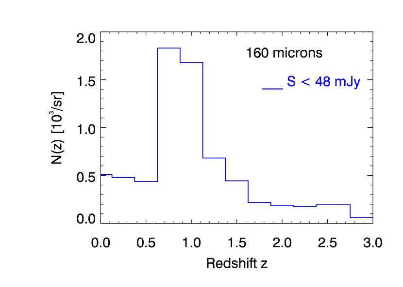
Figure 9: Redshift Distribution of the sources below 48 mJy creating the fluctuations, at 160 $\mu m$ with MIPS. The number of sources is shown for the particular bin sizes.

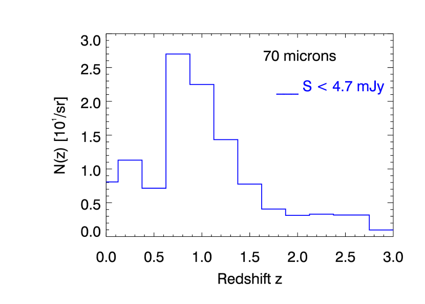
Figure 10: Redshift Distribution of the sources below 4.7 mJy creating the fluctuations, at 70 $\mu m$ with MIPS. The number of sources is shown for the particular bin sizes.

10 Unresolved Sources: Fluctuations of the Cosmic Infrared Background

10.1 Fluctuation Level and Redshift Distributions

Sources below the detection limit of a survey create fluctuations. If the detection limit does not allow to resolve the sources dominating the CIB intensity, characterizing these fluctuations gives very interesting informations on the spatial correlations of these unresolved sources of cosmological significance. The far infrared range is “favored” for measuring the fluctuations, because data are available with very high signal to detector noise ratios, but limited by the confusion; on the other hand, the confusion limits the possibility to detect faint resolved sources and leaves the information about faint sources hidden in the fluctuations. The study of the CIB fluctuations is a rapidly evolving field. After the pioneering work of Herbstmeier et al. (1998) with ISOPHOT, Lagache & Puget (2000) discovered them at 170 $\mu m$ in the FIRBACK data, followed by other works at 170 and 90 $\mu m$ Matsuhara et al. (2000); Kiss et al. (2001); Puget & Lagache (2000), and at 60 and 100 $\mu m$ by Miville-Deschênes et al. (2002) in the IRAS data.

Our model reproduces the measured fluctuation levels within a factor 1.5 between 60 and 170 $\mu m$ Lagache et al. (2002). For MIPS, we predict that the level of the fluctuations is 6930 Jy${}^{2}/sr$ at 160 $\mu m$ for $S_{160}<48$ mJy, and is 113 Jy${}^{2}/sr$ at 70 $\mu m$ for $S_{70}<4.7$ mJy.

Our model gives access to the redshift distribution of the sources dominating the observable fluctuations of the unresolved background. At 170 $\mu m$ (Fig. 12 from Lagache et al. (2002)), the redshift distribution of the contributions to the fluctuations peaks at z=0.8, with a tail up to z $\sim$ 2.5, and there is a non negligible contribution from local sources. This peak of this distribution is similar to the one of the $15\mu m$ ISOCAM redshift distribution of resolved sources Elbaz et al. (2002), which are understood to represent a significant fraction of the CIB. These sources observed at two different wavelengths should tell us the same story about galaxy evolution. The key point of studying the fluctuations in the far infrared is the availability of large area surveys to exhibit the source clustering properties; this is not yet possible with mid infrared data that need to be taken with deeper (and thus less area coverage) exposures to probe the same sources. Furthermore, a non negligible contribution comes from higher redshifts. Extracting this component will be a challenge requiring the use of all SIRTF bands.

At 160 $\mu m$ (Fig. 9), for the same reasons, the distributions of the sources dominating the fluctuations peaks at z=0.8, with a broad peak from z=0.7 to z=1.1. The tail extends up to z $\sim$ 2.5, and the contribution of local sources is less prominent than at 170 $\mu m$ with the ISOPHOT sensitivity. At 70 $\mu m$ (Fig. 10), the distribution is similar to that at 160 $\mu m$, but with a factor of three less source density, since the background is half resolved into sources.

10.2 Power Spectrum Analysis: Fluctuations and Source Clustering

The Poisson component of the fluctuations of the CIB has been detected in the FIR by Lagache & Puget (2000) in the FIRBACK data, at spatial frequencies (or wavenumbers) $0.25<k<0.6$ arcmin^-1. A preliminary study on larger fields seems to show that the source clustering is present in the data as well Puget & Lagache (2000), and are currently under investigation Sorel et al., in prep . However, to accurately constrain the source clustering, larger fields than FIRBACK are needed. Since SIRTF will cover larger sky areas, the clustering should be detected and measured in a power spectrum analysis similar to the one done by Lagache & Puget (2000) and Miville-Deschênes et al. (2002).

We make an estimation of the spatial frequency range where the CIB fluctuations will be detected in the large and shallow surveys at 160 $\mu$m, using our model; it does not include source clustering, we just assume a Poisson distribution of the sources. The detectability of the source clustering is addressed below.

We use the same technique as Lagache & Puget (2000) and Puget & Lagache (2000); following their formalism, the power spectrum measured on the map $P_{map}$, in the space of the detector, can be written as follows:

$$P_{map}=P_{noise}+(P_{cirrus}+P_{sources})\times W_{k}$$ (12)

where $P_{noise}$, $P_{cirrus}$, $P_{sources}$ are the power spectra of the photon/detector noise, the foreground cirrus, and the extragalactic sources we are interested in respectively, and $W_{k}$ is the power spectrum of the PSF. In this analysis, we want to exhibit $P_{sources}$ and, for convenience, $P_{cirrus}$.

Fig. 11 shows a prediction for the various components present at 160 $\mu m$ in a survey like the GTO Shallow or SWIRE. $P_{sources}$, the Poisson component for the fluctuations due to extragalactic sources fainter than 48 mJy is shown as an horizontal line, at the value of 6930 Jy${}^{2}/sr$ predicted by the model (see Sect.10.1). $P_{cirrus}$ is shown as a dash line, and follows a $k^{-3}$ power law Gautier et al. (1992); Miville-Deschênes et al. (2002). The normalization at $10^{6}$ Jy${}^{2}/sr$ at $k=10^{-2}$ arcmin^-1 is typical of the faint cirrus present in the cosmological fields of column density $N_{HI}=10^{20}$ cm^-2. Finally, $P_{noise}/W_{k}$ is plotted as a dot line. The noise is a white noise of $1\sigma$ of 7 mJy, typical for shallow surveys at 160 $\mu m$ (Tab. 5).

To have an estimation of the spatial frequency range where the Poisson fluctuations from the extragalactic component will be detected, one has to consider the two limiting components: galactic cirrus at low spatial frequencies, and photon noise plus PSF shape at large spatial frequencies. It appears that the CIB Poisson fluctuations, or the fluctuations created by faint extragalactic sources only, should be well detected in the wavenumber range $0.07<k<1.3$ arcmin^-1.

Taking into account the source clustering, we assume that it is dominated by starburst galaxies with the form predicted by Perrotta et al. (2001). This clustered component is plotted in Fig. 11 as a dot-dash line, and has been computed for 170 $\mu m$. This component should be detected in the wavenumber range from 0.04 to 0.2 arcmin^-1. The cirrus limits the detection at smaller wavenumbers, and is the main limitation for the source clustering detection. The Poissonian component of extragalactic sources limits the detection at larger wavenumbers.

The large shallow surveys in the FIR are thus the most promising for studying the fluctuations and estimating the source clustering ($0.04<k<0.2$ arcmin^-1).

Figure 11: Theoretical power spectrum of a 5 Sq. Deg. field at 160 $\mu m$, illustrating the spatial frequency range where the CIB fluctuations will be detected (see text Sect. 10.2). Solid line: level of CIB Poisson fluctuations created by sources below 48 mJy predicted by our model: 6930 Jy²/sr. Dash: Foreground Cirrus, $P_{cirrus}$, with the $k^{-3}$ behaviour and normalized at $10^{6}$ Jy²/sr at $k=0.01$ arcmin^-1, representing a column density of $N_{HI}=10^{20}$ cm^-2. Dot: White noise ($1\sigma$ of 7 mJy) divided by the PSF, $P_{noise}/W_{k}$. Dash-Dot: model source clustering of starburst galaxies of Perrotta et al. (2001) in the case of 170 $\mu m$. The wavenumber range of cosmological interest is thus from 0.07 to 1.3 arcmin^-1, where the CIB Poisson fluctuations are expected to be detected; assuming the source clustering has the form predicted by Perrotta et al. (2001), it will be detected in the wavenumber range from 0.04 to 0.2 arcmin^-1.

11 Conclusion

In this work, we review the sources of noise expected in the cosmological surveys to be conducted by MIPS: photon/detector noise, cirrus noise, and confusion noise due to extragalactic sources. Using the Lagache, Dole, & Puget (2002) model, as well as the latest knowledge of the MIPS pre-flight characteristics (in particular the photon/detector noise properties and the beam shapes), we predict the confusion levels, after a detailed discussion on the criteria. In particular, we show that in general the criterion depends on the shape of the source counts and the solid angle of the beam (directly related to the telescope and detector pixel size). SIRTF is about to probe a new regime in the source counts, where a significant fraction of the CIB is resolved and the counts begin to flatten. We thus discuss the classical rules of determining the confusion level (essentially valid for IRAS or ISO), and we show that it is wise to compare the photometric and source density criteria for predicting the confusion level. We found $S_{lim}$ to be 50 $\mu$Jy, 3.2 mJy and 36 mJy at 24, 70 and 160 $\mu m$ respectively, consistent with ISO data or other works.

We compute the final sensitivity of the MIPS surveys, the GTO (guaranteed time) and two Legacy programs (SWIRE and GOODS), predict the number of sources, and give the redshift distributions of the detected sources at 24, 70 and 160 $\mu m$. The deepest surveys should detect the dust emission of sources up to z=2.7 at 24 $\mu m$ (the redshifted 7.7 PAH feature causes a drop of detectability at higher redshifts), and up to z=2.5 at 70 and 160 $\mu m$. This corresponds to a resolution of the CIB into discrete sources of 69, 54 and 24% at 24, 70 and 160 $\mu m$ respectively. We estimate that in the shallow surveys, the sources will be detected in a sufficient number in redshift bins to reconstruct the luminosity function and its evolution with redshift with a 14% (or better) accuracy, as follows: most of the $L>10^{12}L_{\odot}$ in the $0.5\lesssim z\lesssim 1$ in the FIR range and most of the $L>10^{11}L_{\odot}$ in the $0.5\lesssim z\lesssim 1$ in the MIR range, and all the $L\gtrsim\times 10^{13}L_{\odot}$ sources for $z\simeq 2.5$ in the MIR and FIR range. We also show that at 24 $\mu m$, deeper and narrower surveys will considerably increase the sensitivity to lower luminosity galaxies.

We also explore some characteristics of the unresolved sources at long wavelength, among which the redshift distribution of the contribution to the background fluctuations at 70 and 160 $\mu m$. It peaks at $z\sim 0.8$, consistent with our present understanding of the main contribution to the CIB. We estimate the wavenumber range where the large FIR surveys will be able to measure the fluctuations of the Poisson component in a power spectrum analysis is $0.07<k<1.3$ arcmin^-1. With some assumption about the source clustering, we show that it could be detected in the wavenumber range $0.04<k<0.2$ arcmin^-1.

We emphasize the complementary role of large and shallow surveys in the far infrared and smaller but deeper surveys in the mid infrared. The MIR surveys allow to probe directly faint sources, and FIR surveys allow to access the statistical properties of the faint population, mainly through CIB fluctuation analysis. With the various sky area coverage and depth, the MIPS surveys (together with IRAC data helping to estimate the photometric redshifts) will greatly improve our understanding of galaxy evolution by providing data with unprecedented accuracy in the mid and far infrared range.

References

- Altieri et al., (1999) Altieri B. and Metcalfe L. and Kneib J. P.et al. 1999, A&A, 343, L65
- (2) Blaizot, J. et al, in preparation.
- Boulanger et al. (2000) Boulanger, F, Abergel, A, Cesarsky, D, Bernard, J. P, Miville-Deschênes, M. A, Verstraete, L, & Reach, W. T. Small dust particles as seen by iso. In R. J. Laureijs, K. L & Kessler, M. F, editors, ISO Beyond Point Sources: Studies of Extended Infrared Emission, page 91, ISO Data Centre, Villafranca del Castillo, Madrid, Spain, 2000.
- Boulanger (2000) Boulanger, F. Studies of diffuse infrared emission. In R. J. Laureijs, K. L & Kessler, M. F, editors, ISO Beyond Point Sources: Studies of Extended Infrared Emission, page 3, ISO Data Centre, Villafranca del Castillo, Madrid, Spai, 2000.
- Chary & Elbaz (2001) Chary, R & Elbaz, D. 2001, ApJ, 556:562.
- Condon (1974) Condon, J. J. 1974, ApJ, 188:279.
- Devriendt & Guiderdoni (2000) Devriendt, J. E. G & Guiderdoni, B. 2000, A&A, 363:851.
- Dole et al. (2000) Dole, H, Gispert, R, Lagache, G, Puget, J. L, Aussel, H, Bouchet, F. R, Ciliegi, P, Clements, D. L, Cesarsky, C. J, Désert, F. X, Elbaz, D, Franceschini, A, Guiderdoni, B, Harwit, M, Laureijs, R, Lemke, D, Moorwood, A. F, Oliver, S, Reach, W. T, Rowan-Robinson, M, & Stickel, M. Firback source counts and cosmological implications. In Lemke, Stickel, W. e, editor, ISO view of a Dusty Universe, Ringberg, Nov 1999, astro-ph/0002283. Springer Lecture Notes, 2000.
- Dole et al. (2001) Dole, H, Gispert, R, Lagache, G, Puget, J. L, Bouchet, F. R, Cesarsky, C, Ciliegi, P, Clements, D. L, Dennefeld, M, Désert, F. X, Elbaz, D, Franceschini, A, Guiderdoni, B, Harwit, M, Lemke, D, Moorwood, A. F. M, Oliver, S, Reach, W. T, Rowan-Robinson, M, & Stickel, M. 2001, A&A, 372:364.
- Elbaz et al. (2002) Elbaz, D, Cesarsky, C. J, Chanial, P, Aussel, H, Franceschini, A, Fadda, D, & Chary, R. R. 2002, A&A, 384:848.
- Engelbracht et al. (2000) Engelbracht, C. W, Young, E. T, Rieke, G. H, lis, G. R, Beeman, J. W, & Haller, E. E. 2000, Experimental Astronomy, 10:403.
- Fazio et al. (1998) Fazio, G. G, Hora, J. L, Willner, S. P, Stauffer, J. R, Ashby, M. L, Wang, Z, Tollestrup, E. V, Pipher, J. L, Forrest, W. J, McCreight, C. R, Moseley, S. H, Hoffmann, W. F, Eisenhardt, P, & Wright, E. L. Infrared array camera (irac) for the space infrared telescope facility (sirtf). In Fowler, A. M, editor, Infrared Astronomical Instrumentation, page 1024, 1998.
- Franceschini et al. (1989) Franceschini, A, Toffolatti, L, Danese, L, & De Zotti, G. 1989, ApJ, 344:35.
- Franceschini et al. (1991) Franceschini, A, Toffolatti, L, Mazzei, P, Danese, L, & De Zotti, G. 1991, A&As, 89:285.
- Franceschini et al. (2001) Franceschini, A, Aussel, H, Cesarsky, C. J, Elbaz, D, & Fadda, D. 2001, A&A, 378:1.