Planets in habitable zones:

The recently discovered planetary system in the binary $\gamma$ $Cep$ was studied concerning its dynamical evolution. We confirm that the orbital parameters found by the observers are in a stable configuration. The primary aim of this study was to find stable planetary orbits in a habitable region in this system, which consists of a double star (a=21.36 AU) and a relatively close (a=2.15 AU) massive ($1.7$ $m_{jup}$ $\sin i$) planet. We did straightforward numerical integrations of the equations of motion in different dynamical models and determined the stability regions for a fictitious massless planet in the interval of the semimajor axis $0.5$ AU $<a<$ $1.85$ AU around the more massive primary. To confirm the results we used the Fast Lyapunov Indicators (FLI) in separate computations, which are a common tool for determining the chaoticity of an orbit. Both results are in good agreement and unveiled a small island of stable motions close to 1 AU up to an inclination of about $15^{o}$ (which corresponds to the 3:1 mean motion resonance between the two planets). Additionally we computed the orbits of earthlike planets (up to 90 earthmasses) in the small stable island and found out, that there exists a small window of stable orbits on the inner edge of the habitable zone in $\gamma$ $Cep$ even for massive planets.

1 Introduction

Extra solar planets exist also in double stars and, due to the fact that double and multiple star systems are more numerous than single stars, we expect many more discoveries in such systems in future. All of the five systems (table 1) with planetary companions are of the so-called S-type, where the planet orbits one primary. This type of motion was studied theoretically since more than 20 years (see e.g. Dvorak 1984 and 1986, Rabl & Dvorak 1988, Holman & Wiegert 1999, Pilat-Lohinger 2000a and 2000b, Pilat-Lohinger & Dvorak 2002). Stability studies have been undertaken for the other type of motion in binaries, the P-type, where the planet orbits both components of a binary (see e.g. Goudas 1963, Dvorak et al. 1989, Holman & Wiegert 1999, Broucke 2001, Pilat-Lohinger et al. 2002), but up to now we do not have evidence that they exist. From the cosmogonic point of view the S-types may have formed similar to a planet around a single star.

Table 1: Exoplanets in binaries

Star	Planet	$M\sin i$	a	e	period
		[$M_{J}$]	[AU]		[days]
Gliese 86	Gl86 b	4	0.11	0.046	15.78
(K1 V)
55 Cancri	55Cnc b	0.85	0.115	0.02	14.653
(G8 V)	55Cnc c	0.21	0.241	0.339	44.275
	55Cnc d	4.95	5.9	0.16	5360
16 Cyg B	16CygB b	1.5	1.72	0.67	804
(G2.5 V)
$\tau$ Bootis	$\tau$Boo b	4.09	0.05	0.	3.312
(F7 V)
$\gamma$ Cephei	$\gamma$Cep b	1.76	2.15	0.209	903
(K1 IV)

The recently discovered Jupiter size planet in HD 222404 ($\gamma$ $Cep$) (see Cochran et al, 2002) has a slightly eccentric orbit in a mean distance of $a=2.15$ AU around the K1 IV star (table 2). Our study shows the dynamical stability of this planetary orbit with the published orbital parameters. The main subject of our investigations is the existence of possible planets in the habitable region in a wider sense between $0.5$ AU $<a<1.85$ AU from the point of view of orbital dynamics.

Table 2: The $\gamma$ $Cep$ planetary system

	Star A	Star B	Planet
Temperature [K]	4900	3500	—
Radius [Solar Radii]	4.7	0.5	—
Mass [Solar masses]	1.6	0.4	0.00168
Period [years]		70	2.47
Semi-major Axis [AU]		21.36	2.15
Eccentricity		0.44	0.209

2 Numerical setup and dynamical model

The equations of motion were integrated with two different methods:

1. We used the Lie-integrator (see e.g. Hanslmeier and Dvorak 1984, Lichtenegger 1984) specially adapted for these problems. It uses an automatic step size and can quite precisely integrate also high eccentric orbits. The time interval of computation for the Lie-integration was set to 1 million years (which corresponds to approx. $1.5\times 10^{4}$ periods of the primaries). The stability definition for the orbits was the following: An orbit is stable up to the moment when a “possible crossing of the orbits” occurs, which means that the massive planet’s periastron and the fictitious planet’s apoastron allow close encounters.

2. The Bulirsch-Stoer integrator was used in connection with the computation of the Fast Lyapunov Indicators (FLIs) (see Froeschlé et al. 1997); this is a well known tool to distinguish between chaotic and regular orbits. The computations of the FLIs were carried out for $10^{4}$ binary periods. To determine the stable motion we defined a critical value for the FLIs (i.e. $10^{9}$), up to which all orbits were found to be regular.

The following dynamical models were investigated:

model A: The simplest dynamical model, where one can explore the stability of a planet in a binary, is the elliptic restricted three body problem; the planet’s mass is neglected– thus the binary describes an unperturbed Keplerian motion. This model was used for all studies cited in the introduction above.

model B: In the “restricted four-body problem” (binary + massive planet + massless fictitious planets) we checked the orbits in the region inside the orbit of the planet (0.5 AU to 1.85 AU)

model C: The most realistic model for this system is a full 4-body problem where the inner – fictitious – planet has also a mass, which we varied in the following way: $m_{earth}\leq m\leq 90$ $m_{earth}$.

In the framework of these three dynamical models we integrated the orbits of tenthousands of fictitious massless planets (and hundreds of massive planets) for a different grid of semimajor axes and we varied also the orbital inclination of the additional planet (the initial orbit was always circular).

3 The stability of the planet in $\gamma$ Cep

Using the parameters of the binary given in table 2 we found for a massless regarded planet a large zone of stability (fig. 1). For different eccentricities of the binary and also of the planet ($0<e<0.5$) we computed a diagramm of possible stable orbits for the mass ratio $\mu=m_{B}/(m_{A}+m_{B})=0.2$ . The calculations for this study were done in the dynamical model A, (the elliptic restricted three body problem) which does not take into account a possible inclination of the planet’s orbit. For the present configuration (the eccentricities of the binary $e=0.4$ and the planet $e=0.2$) the planet is in a very stable zone and could be stable up to almost twice its observed semimajor axes $a<4$ AU. When we use theoretical results of the stability of P-types (see e.g. Pilat-Lohinger et al. 2002, and references therein) we believe that even an inclined orbital plane of the planet’s motion would not fundamentally change this diagramm.

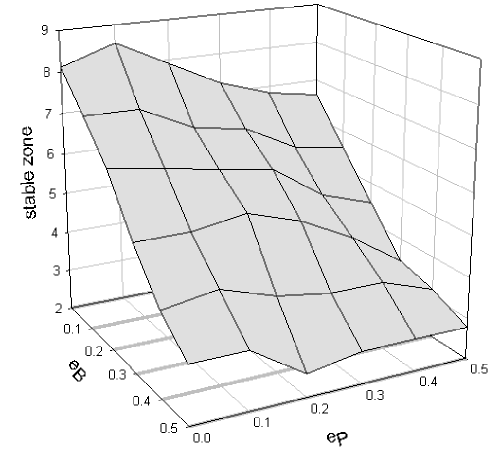
Figure 1: The limits in AU of the stable zone for (z-axis) for the mass ratio $\mu=0.2$ of $\gamma$ $Cep$, where the initial eccentricities of the planet (x-axis) and of the binary (y-axis) vary from 0 to 0.5

4 Planets in habitable zones

With a grid of $\Delta a=0.05$ between 0.5 AU and 1.85 AU we did computations of the orbits of fictitious massless planets in model B and also took into account possible inclinations of the plane of motion of the planet in this region ($\Delta i=5^{o}$ for $0^{o}<i<50^{o}$). Fig. 2 shows the escape regions according to their escape times determined with the Lie-integration. The dark regions are the ones were the planet escapes after a very short time and reaches an eccentricity which allows close encounters between the “real” planet and the fictitious one, the white regions show the stable orbits (within the time of integration). We can see the increase of the regions of stable orbits with larger inclinations, which is well understood from the geometry of the different orbits which unables encounters for inclined orbits. The most interesting feature is the stable region around 1 AU for the planar orbits, which extends up to $i=10^{o}$, then disappears and reappears for larger inclinations ($i>30^{o}$). The larger unstable zone between $40^{o}$ and $50^{o}$ is probably due to the acting Kozai resonance (Kozai, 1962).

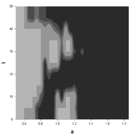
Figure 2: Stability regions for $\gamma$ $Cep$; semimajor axis in AU (x-axis) versus inclination. Only the light grey regions indicate stable orbits, the different darker grey tones show the escape times in decreasing order; black marks a fast escape within 10 periods of the binary

To check the rôle of the eccentricity of the known planet on the size of the stability regions, we made two more computations in model B in the planar problem: for $e=0.1$ we discovered an increase of the stable region up to $a=1.4$ AU. For $e=0.3$ the stable region extends only up to 0.65 AU without any stable window in the unstable zone! Such an eccentric orbit does not allow a planet orbiting in a habitable region in $\gamma$ $Cep$.

We repeated the study using the FLIs, but now we integrated for a slightly shorter time because this chaos indicator is quite effective even for short time integrations. Because the method is also faster, we used a finer grid for the semimajor axis ($\Delta a=0.01$) and also for the inclination ($\Delta i=1^{o}.7$). The results of the FLIs shown in fig. 3 correspond quite well to fig. 2 although more details are visible: the stable region around 1 AU (3:1 resonance) is much smaller, but it also extends up to an inclination of approximately $15^{o}$. This island of stability lies in a large region of unstable motion, which becomes smaller with larger inclinations of the planets’ orbit. The tiny islands of different grey indicate different values of the FLI.

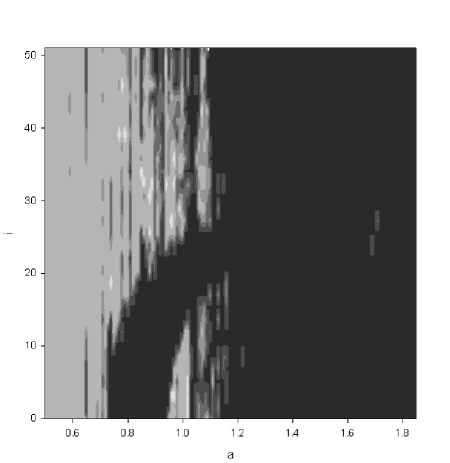
Figure 3: Stability diagramm for $\gamma$ $Cep$ derived with the FLIs; semimajor axis in AU (x-axis) versus inclination. The different shades corresponds to different values of the FLI, which splits up the phase space into different types of motion: from light grey (stable) to black (chaotic). The latter corresponds to the unstable zone in fig. 2.

Additionally we checked with the Lie-integration the region around 1 AU (for $i=0$) in the planar problem with separate computations for a finer grid ($\Delta a=0.02$). We confirmed the results of the FLIs (see fig. 3) which show the complicated structure in this region close to the 3:1 mean motion resonance, where also high order resonances and secondary resonances are present.

5 Massive planets in the habitable zone

The next problem to study was how a terrestrial planet may influence the orbit of the discovered planet. We started the test computation in the “stable window” which we discovered close to 1 AU with masses of the fictitious planet $m_{earth}<m<15$ $m_{earth}$ and with a grid of $\Delta a=0.02$ AU but did not take into account a possible inclination of the fictive planets’ orbit. In fig. 4 we show the results and indicate escaping orbits (dark), unstable orbits (grey) and stable orbits (white). It is remarkable that only for a = 1 AU all orbits for the different masses of the fictitious planet are stable. The comparison of the stability for a ”massless” planet with massive planets shows, that there are differences, but the stability window is still present although the structure changes. Test calculation for larger masses of the additional planet close to a = 1 AU showed, that there are still stable orbits up to m = 90 earthmasses. Another interesting fact is, that we found “jumping orbits”; this means, that the semimajor axis jumps on a very small scale irregularly between two different values (corresponding to very close high order resonances inside the 3:1 mean motion resonance). This phenomenon was recently found for another extrasolar planetary system namely for HD 12661 (see Kiseleva-Eggleton et al. 2002) and is very probable due to a jumping between high order resonances as it was found by Milani et al. (1989).

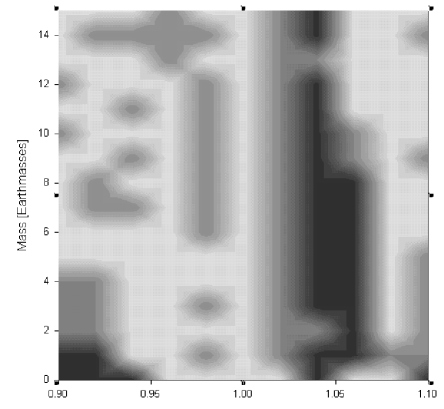
Figure 4: Stability diagramm for $\gamma$ $Cep$ initial distance (x-axis) versus the mass of a fictitious planet in Earthmasses (y-axis)

Figure 5: A jumping orbit for a fictitious planet ($m=2m_{earth}$) in $\gamma$ $Cep$ for 1 million years

6 Conclusions

In this study we confirm the dynamical stability of the recently discovered planet in the binary $\gamma$ $Cep$ over at least some $10^{8}$ years, which let us assume that the orbital parameters found by the observers are in a stable configuration up to cosmogonically time scales. Therefore the primary aim of our investigations was to find stable planetary orbits in a habitable region in this system. Due to the results of extensive numerical experiments, for which we used direct integrations and also the FLIs, we discovered, that there could exist planets in the stability regions depending on the inclination of the orbit of the fictitious planet inside the orbit of the known planet. We unveiled the existence of a small island of stable motions close to 1 AU up to an inclination of about $15^{o}$ (3:1 mean motion resonance between the two planets). Final calculations with massive earthlike planets (up to 90 Earthmasses) in the small stable island confirm, that even for massive planets there exists a small window of stable orbits on the inner edge of the habitable zone in $\gamma$ $Cep$.

- (1) Broucke, R.A. 2001 CMDA, 81, 321.
- (2) Cochran W.D., Hatzes A.P., Endl M., Paulson D.B., Walker G.A.H., Campbell B., Yang S., 2002, AAS #34,#42.02
- (3) Dvorak R., 1984, CMDA, 34, 369
- (4) Dvorak R., 1986, A&A 167, 379
- (5) Dvorak R., Froeschlé Ch. and Froeschlé C., 1989, A&A, 226, 335
- (6) Froeschlé C., Lega E. and Gonczi R., 1997, CMDA, 67, 41
- (7) Goudas, C.L. 1963 Icarus, 2, 1
- (8) Hanslmeier A. and Dvorak R., 1984, A&A, 132, 203
- (9) Hadjidemetriou, J, 2002, CMDA, 83, 141
- (10) Holman M.J., Wiegert P.A., 1999, AJ, 117, 621
- (11) Kasting, J.F., Whitmire, D.P. and Reynolds, R.T., 1993, Icarus, 101, 108
- (12) Kiseleva-Eggleton, L., Bois, E., Rambaux, N. and Dvorak, R., 2002, ApJ , 578, L145
- (13) Kozai, Y., 1962, AJ , 67, 591
- (14) Lichtenegger H., 1984, CMDA, 34, 357
- (15) Milani, A., Carpino, M., Hahn, G. and Nobili, A.M., 1989, Icarus, 78, 212
- (16) Pilat-Lohinger E., 2000a, Proceedings of the Alexander von Humboldt Colloquium on Celestial Mechanics ed. Dvorak R. & Henrard J., Kluwer Academic Publisher, 329
- (17) Pilat-Lohinger E., 2000b, Proceedings of the Austrian Hungarian Workshop on Trojans and related Topics, ed. Freistetter F., Dvorak R. & Erdi B., Eötvös University Press, 77
- (18) Pilat-Lohinger E. and Dvorak R., CMDA, 82, 143-153, 2002.
- (19) Pilat-Lohinger E., Funk B. and Dvorak R., A&A, 2002, in press
- (20) Rabl G. and Dvorak R., A&A, 191, 385-391, 1988