The He-shell flash in action: T Ursae Minoris revisited

We present an updated and improved description of the light curve behaviour of T Ursae Minoris, which is a Mira star with the strongest period change (the present rate is an amazing $-3.8\pm$0.4 days/year corresponding to a relative decrease of about 1% per cycle). Ninety years of visual data were collected from all available databases and the resulting, almost uninterrupted light curve was analysed with the O$-$C diagram, Fourier analysis and various time-frequency methods. The Choi-Williams and Zhao-Atlas-Marks distributions gave the clearest image of frequency and light curve shape variations. A decrease of the intensity average of the light curve was also found, which is in accordance with a period-luminosity relation for Mira stars. We predict the star will finish its period decrease in the meaningfully near future (c.c. 5 to 30 years) and strongly suggest to closely follow the star’s variations (photometric, as well as spectroscopic) during this period.

1 Introduction

During the last several years, there has been an increasing number of Mira stars discovered to show long-term continuous period changes (see some recent examples in Sterken et al. 1999, Hawkins et al. 2001 and a comprehensive reanalysis of R Hydrae, an archetype of such Mira stars, by Zijlstra et al. 2002). The widely adopted view of their period change is based on the He-shell flash model, outlined by Wood & Zarro (1981). According to this model, energy producing instabilities appear when a helium-burning shell, developed in the early Asymptotic Giant Branch (AGB) phase, starts to exhaust its helium content. Then the shell switches to hydrogen burning, punctuated by regular helium flashes, called also as thermal pulses (Vassiliadis & Wood 1993). During these flashes the stellar luminosity changes quite rapidly and the period of pulsation follows the luminosity variations.

Rapid period decrease in T Ursae Minoris (= HD 118556, V${}_{\rm max}\approx 9\aas@@fstack{m}0$, V${}_{\rm min}\approx 14\aas@@fstack{m}0$) was discovered by Gál & Szatmáry (1995), who analysed $\sim$45 years-long visual data distributed in two distinct parts between 1932 and 1993. Mattei & Foster (1995) analysed almost 90 years of AAVSO data collected between 1905 and 1994 and concluded that the period decreasing rate of T UMi (2.75 days/year as determined by them) is twice as fast as in two other similar Mira stars (R Aql and R Hya). Most recently, Šmelcer (2002) presented almost three years of CCD photometry of T UMi, resulting in four accurate times of maximum.

The main aim of our paper is to update our knowledge on T UMi. The eight years passed since the last two detailed analyses witnessed a considerable development in time-frequency methods, which allow more sophisticated description of light curve behaviour. On the other hand, these eight years yielded more than 10 new cycles of the light curve prolonging quite significantly the time-base of the period decreasing phase. The paper is organised as follows. Observations are described in Sect. 2, a new and more sophisticated light curve analysis is presented in Sect. 3. Results are discussed in Sect. 4.

2 Observations

Four sources of visual data were used in our study. The bulk of the data was taken from the publicly available databases of the Association Française des Observateurs d’Etoiles Variables (AFOEV) and the Variable Star Observers’s League in Japan (VSOLJ). (Besides the visual data, the AFOEV subset contains a few CCD-V measurements, too.) Since these data end in early 2002, the latest part of the light curve is covered via the VSNET computer service. The merged dataset showed a quite large gap between JD 2431000 and 2437000. Therefore, we have extracted data collected by the American Association of Variable Star Observers (AAVSO) with help of the Dexter Java applet available at the Astrophysical Data System (these data were published by Mattei & Foster (1995) as light curves, which can be converted into ASCII data with that Java applet). Basic data of individual sets are summarized in Table 1.

Table 1: A summary of the analysed datasets (MJD=JD$-$2400000).

Source	MJD(start)	MJD(end)	No. of points
AFOEV	22703	52457	4073
AFOEV(CCD)	51071	52321	271
VSOLJ	36691	52273	891
VSNET	49925	52551	501
AAVSOa	20043	49530	3213

^a Mattei & Foster (1995)

We found the different data to agree very well (similarly to the case of R Cygni in Kiss & Szatmáry 2002) and that is why we simply merged the independent observations to form the final dataset. It is almost uninterrupted between 1913 and 2002 and consists of 8949 individual magnitude estimates (negative (“fainter than…”) observations were excluded). We have calculated 10-day means and this binned light curve was submitted to our analysis. It is shown in Fig. 1, where the close agreement of simultaneous CCD-V and visual observations supports the usability of the latter data (some tests and comparisons of photoelectric and visual observations can be found in Kiss et al. 1999 and Lebzelter & Kiss 2001).

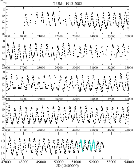
Figure 1: The whole dataset of T UMi (10-day means). Light gray points in the bottom panel refer to CCD-V measurements collected by the AFOEV.

3 Light curve analysis

3.1 The $O-C$ diagram

To construct the classical O$-$C diagram, we determined all times of maximum from the binned light curve. This was done partly by fitting low-order (3–5) polynomials to selected parts of the light curve, partly by simple ‘eye-ball’ estimates of the epochs of maximum from computer generated plots. The latter was chosen when the scatter of the curve and/or loose sampling did not permit reliable fitting. We could determine 106 observed epochs (with estimated errors of $\pm$5 and $\pm$10 days), i.e. only very few cycles were lost between 1913 and 2002. Eight additional times of maximum was provided by J. Percy (1994, personal communication), which were observed between 1907 and 1913. Therefore, the full set consists of 114 observed maxima with a time-base of 95 years. To allow an easy comparison with Fig. 4 in Gál & Szatmáry (1995), we plot the resulting O$-$C diagram with the same ephemeris ($JD_{\rm max}=2416971+313.42\cdot E$) in Fig. 2.

Obviously the star continued the period decrease at an amazing rate. A close-up to the last part of the O$-$C diagram revealed its very parabolic nature indicating constant rate of period change (similar conclusion was drawn by Šmelcer 2002). By fitting a parabola to the last 7500 days, we determined the second-order coefficient as $(-1.82\pm 0.18)\cdot 10^{-5}$ days/days. Using the expression for this coefficient in terms of period and period changing rate ($\frac{1}{2}\frac{1}{P}\frac{dP}{dt}$, Breger & Pamyatnykh 1998), we obtained a relative rate of $(1/P)dP/dt=(-3.6\pm 0.36)\cdot 10^{-5}$ days/days. Here $P$ stands for the period in the ephemeris used to construct the O$-$C diagram, hence the period derivative $dP/dt$ equals to $-4.2\pm 0.4$ days/year.

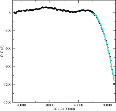
Figure 2: The O$-$C diagram of T UMi. The solid line is the parabolic fit of the last 7500 days.

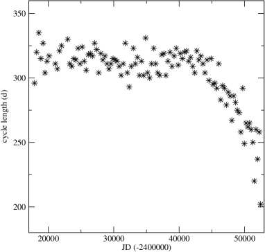
Figure 3: The cycle length as a function of time.

The rate of period decrease was also determined from the individual cycle lengths. They are plotted as a function of time in Fig. 3. There is a well-expressed break at JD 2444000 and since then the period has decreased fairly linearly, although some curvature cannot be excluded either. By fitting a linear regression to the last 7500 days, we arrived to a similar result: $dP/dt=3.4\pm 0.5$ days/year. This is about the same than that of Šmelcer (2002) who gave 3.1 days/year. In summary, we adopt the simple mean of the two values which is $dP/dt=3.8\pm 0.4$ days/year. Presently it corresponds to about 1 percent relative decrease per cycle! To our knowledge, there is only one star with similarly fast gradual period change among all types of pulsating stars (sudden period changes due to mode switching phenomenon are not considered here): BH Crucis, which is another Mira star but with period increase (Zijlstra & Bedding 2002). Its period has increased since 1975 from 420 to 530 days, i.e. with an approximate rate of about 4 days/year. Whatever the reason is, these stars are obviously very peculiar members of their class (see Percy & Au 1999 for a search for evolutionary period changes in 391 Mira stars).

3.2 Fourier analysis and time-frequency distributions

Fourier and time-frequency analyses make use of the full light curve, not only special points, thus their application usually reveals a lot more information on the light variation.

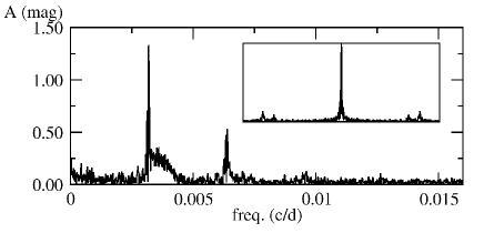
Figure 4: The frequency spectrum of T UMi with the window function in the small insert. The frequency scale is the same for both graphs.

First, we calculated the frequency spectrum of T UMi with Period98 (Sperl 1998). It is plotted in Fig. 4, where the window function is also shown in the small insert. The shape of the spectrum around the dominant peak is very characteristic for a signal with continuously changing frequency. The second and third harmonics (due to the asymetric light curve shape) are easily visible and there is a slight indication for the fourth harmonic, too. Thanks to the almost uninterrupted light curve, the window function is free of strong alias structure, only the weak yearly alias and a stronger $1/P$ alias are present (the latter one is caused by a few unobserved minima in the early decades of data).

However, as has been recently demonstrated by numerous studies (e.g. Szatmáry et al. 1996, Foster 1996, Kolláth & Buchler 1996, Bedding et al. 1998, Kiss et al. 2000, Zijlstra et al. 2002), time-frequency analysis utilizing wavelets and other distributions (Cohen 1995) reveals many delicate details undetectable with simple methods.

Figure 5: Three time-frequency distributions. Top panel: wavelet map; middle panel: Choi-Williams distribution (CWD); bottom panel: Zhao-Atlas-Marks distribution (ZAMD).

We calculated several distributions with many different parameter sets with the software package TIFRAN (TIme FRequency ANalysis) developed by Z. Kolláth and Z. Csubry at Konkoly Observatory, Budapest (Kolláth & Csubry 2002). Besides the wavelet map, we present the Choi-Williams (Choi & Williams 1989) and Zhao-Atlas-Marks (Zhao et al. 1990) time-frequency distributions for the whole dataset of T UMi in three panels of Fig. 5. For an easy comparison we also plotted the light curve at the top of the figure and three copies of the Fourier spectrum on the right hand side of the distributions. In order to enhance the visibility of harmonic components, we divided the time-frequency plane in three sections defined by their frequency limits. We chose 0–0.0048 d^-1, 0.0048–0.0096 d^-1 and 0.0096–0.015 d^-1. This selection provided that the fundamental frequency ($f_{0}$), and its second ($2f_{0}$) and third ($3f_{0}$) harmonics fall into different sections. Then we multiplied the amplitude values in these sections by one, two and three, with the larger frequency the larger multiplicator. Detailed experiments were performed with different kernel-parameters $\alpha$ (Buchler and Kolláth 2001), which defines the tradeoff between time resolution and frequency resolution. In the presented cases for the wavelet transform, CWD and ZAMD we used $\alpha$ values of 2.0, 2.0 and 0.2, respectively.

We could draw a few interesting conclusions based on Fig. 5. Both the CWD and ZAMD give much clearer images of the time-dependent frequency content than the wavelet map. Even the fourth harmonic is visible, although with some ambiguity. The light curve shape (defined by the relative strength of the harmonics) changed a lot even in the first part of the data, in which the period remained constant. When the period decrease started (around JD 2444000 or 1979), the harmonics followed the fundamental frequency for $\sim$5000 days but around JD 2449000 they suddenly disappeared – the star became “tuned out”. Consequently, the light curve shape turned to be more sinusoidal. Between 1913 and 1979 we did not find any significant frequency change, only the amplitude of the fundamental and first harmonic seems to show some alternating changes. In order to decide whether they are real changes or only results of the data distribution, we performed a similar test calculation as in Szatmáry et al. (1996). It consisted of creating a wavelet map of the original dataset (‘star’) and another map from a synthesized light curve (‘fit’) calculated with the two dominant frequency components in the Fourier spectrum. The fit-map shows the amplitude variations caused by the gaps and data distribution. A comparison of the star-map with the fit-map (in sense of star minus fit) reveals real amplitude variations.

We show the results in Fig. 6. Here A_i (i=0,1) stands for the star$-$fit difference for the peak amplitudes in the corresponding frequency ranges at any given time. The decrease of the first harmonic after the start of the period decline is quite obvious. There are several occasions when A₀ and A₁ showed alternation but that was not a strict rule. If the star was pulsating in fundamental mode, then the reason for this complex behaviour might be some resonance between the fundamental and first overtone modes, for which a ratio near 2.0 is expected in red giants models (e.g. Ostlie & Cox 1986).

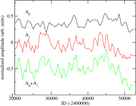
Figure 6: Amplitude variations of the fundamental (A₀) and first harmonic frequencies (A₁).

4 Discussion

We have investigated several aspects and implications of the presented light curve behaviour. An intriguing question is whether the overall luminosity drop expected from the assumption of a period-luminosity (P-L) relation can be detected. This question was addressed by Zijlstra et al. (2002) for R Hydrae, whose period decreased from 495 days to 380 days between 1700 and 1950. These authors examined different assumptions, including luminosity decrease from a P-L relation (Feast 1996), evolution at constant $L$ and even evolution with slightly increasing $L$. From the visual light curve it was concluded that no luminosity change can be proven as the average visual magnitude has not changed since 1910. However, they noted the decreased visual amplitude explained by the non-linearity of pulsation (cf. Kiss et al. 2000 discussing the period-amplitude relation for Y Persei). A similar amplitude decrease was described for another He-shell flash Mira, R Centauri (Hawkins et al. 2001).

However, we feel it necessary to point out that for a large amplitude Mira star one has to be careful when concluding the luminosity constancy from the constant average magnitude. This is because of the logarithmic nature of the magnitude scale. As an illustration, let us consider two Mira stars with $m_{\rm 1,max}=7$ mag, $m_{\rm 1,min}=13$ mag, $m_{\rm 2,max}=8$ mag and $m_{\rm 2,min}=12$ mag. The average magnitude is 10 mag in both cases. However, the physically relevant parameter is the intensity being $i\sim 10^{-0.4m}$. After calculating average intensities, one can convert them to meaningful average magnitudes, in our cases to 7$\aas@@fstack{m}$75 and 8$\aas@@fstack{m}$73. The difference is almost one magnitude. This is a fairly trivial consideration but it has to be kept in mind when averaging large amplitude Mira light curves.

As expected, both R Hya and R Cen showed such amplitude decrease that resulted in fainter maxima and brighter minima (Figs. 1 in Hawkins et al. 2001 and Zijlstra et al. 2002). We found a similar behaviour for T UMi, too, which has already been predicted by Whitelock (1999). To take into account the necessity of intensity averaging, we have converted the binned light curve to intensities and calculated mean intensities per cycles (Fig. 7). The scatter in Fig. 7 is, of course, quite large, due to typical cycle-to-cycle changes of the maximum brightness. However, there is an indication at the end of data for a slight decrease of the intensity. A simple linear fit of the last 7500 days (JD 2445000–2452500) was used to infer $\Delta\langle m\rangle=-0\aas@@fstack{m}47\pm 0\aas@@fstack{m}4$. This value was compared with calculated absolute magnitude changes (see next paragraph). The general appearance of the intensity average curve as a function of time reminded us the shape of the O$-$C diagram and that is why we added the O$-$C points (before JD 2445000) in Fig. 7. The parallel trends suggest that there is a positive correlation between the full intensity and corresponding cycle length.

As a rough approximation, we assumed that averaging along the full cycle smooths out the effects of varying bolometric correction and the mean magnitude difference found from the observations corresponds directly to $\Delta M_{\rm bol}$. Adopting a period change from 315 days to 215 days, the P-L relation derived from LMC Mira stars (Feast 1996)

$$M_{\rm bol}=-3.00\log P+\alpha$$

gives $\Delta M_{\rm bol}=-0\aas@@fstack{m}49$. The close agreement is probably pure coincidence, though remarkable.

Another comparison was made with theoretically expected luminosity change as discussed in Wood & Zarro (1981) when deducing their Eq. (10). From that relation it follows that the luminosity change depends only on the period change and two ambiguosly determined constants ($b$ and $\beta$ in their notation). For $\beta=16.67$ and $b=1.5$ or $2$, we calculated $\Delta M_{\rm bol}=-0\aas@@fstack{m}45$ and $-0\aas@@fstack{m}34$. The agreement is again demonstrative. Therefore, we conclude that the tenuous intensity decrease is consistent (at least partly) with the assumption of P-L relation being applicable in this case. Another effect with similar outcome is the amplitude reduction due to the non-linearity of pulsation. The most likely scenario is that both processes occur in T UMi.

Fig. 3 in Wood & Zarro (1981) led Gál & Szatmáry (1995) to conclude that T UMi is just after the onset of a He-shell flash and it is likely to have core mass similar to R Aql and R Hya. Presently available data shift the core mass to a slightly larger value (between 0.69 and 0.78 $M_{\odot}$), because the most recent $dL/dt$ suggest a steeper function than that for R Hya in Fig. 3 of Wood & Zarro (1981). Adopting those calculations, we estimated some basic parameters of the star. The logarithm of the luminosity for the larger core mass is about 4.2$\pm$0.1 (i.e. $L/L_{\odot}=15800^{+4000}_{-3300}$). That means $M_{\rm bol}=-5\aas@@fstack{m}8\pm 0\aas@@fstack{m}3$ corresponding to a spectral type of M4 II with $M_{\rm V}=-3\aas@@fstack{m}1\pm 0.3$ (Straižys & Kuriliene 1981). This results in a distance of 3.6$\pm$0.5 kpc (interstellar reddening neglected). The definition of luminosity and the assumption of a typical red giant temperature $T_{\rm eff}=3000\pm 200$ K yields $R/R_{\odot}=450\pm 80$. This large radius suggests first overtone pulsation for T UMi (van Belle et al. 2002). On the other hand, period-gravity relation of radially pulsating stars (Fernie 1995) and its extension toward red giant pulsators, mainly semiregular variables (Szatmáry & Kiss 2002) suggest for fundamental and first overtone pulsation $\log\leavevmode\nobreak\ g=-0.22$ and $-0.52$, respectively. The corresponding masses are 4.6 $M_{\odot}$ and 2.3 M_⊙, the former being too large for a Mira star. Tabulated model calculations by Fox & Wood (1982) for similar physical parameters and first overtone periods near 310 days give second overtone periods between 210 and 240 days, close to the presently observable value. Another possibility is that the continuous period change is due to a mode switching phenomenon acting similarly than the pop. II models in type-1 instability region calculated by Bono et al. (1995). Although those models addressed transient phenomena in RR Lyr and BL Her stars, type-1 instability (mode switching from the fundamental to the first overtone mode with continuously changing period – see Fig. 2 in Bono et al. 1995) is roughly similar to the observed behaviour of T UMi.

Either mode change or He-shell flash is acting in T UMi, present large period changing rate suggests that the decrease will stop in the meaningfully near future, between 5 to 30 years from now (i.e. to keep the period in a physically reasonable range). Furthermore, if the He-shell flash model is true and the star is indeed just after the onset of a flash, a similarly rapid period increase can be predicted right after reaching the period minimum. Therefore, it is of paramount importance to follow the star’s variations with as much instrumentation as possible. The average cycle length now is between 200 and 220 days and the rapid decrease implies that the end of the decline is quickly approaching (Zijlstra et al. 2002 found for R Hya that its period showed a c.c. 10% decrease in two decades before ending the period changing phase). In this phase we suggest to try to measure directly the luminosity change (if we accept its existence) via accurate spectrophotometry or high-resolution spectral synthesis. Visual data are crucial for prompt detection of period stabilization or even period increase. The latter would be the final argument confirming the concept of the He-shell flash. However, if the period will turn to a constant value and remains there for a considerable time then the whole theory should be revised. In that case T UMi shall shed new light on a peculiar mode switching phenomenon not well understood.

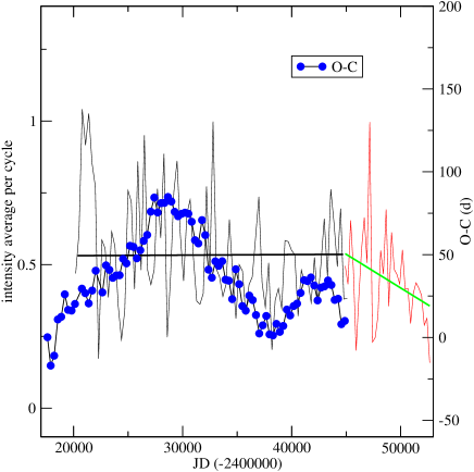
Figure 7: The intensity average per cycle against time and the O$-$C variation before the period decrease.

- (1) Bedding, T. R., Zijlstra, A. A., Jones, A., & Foster, G. 1998, MNRAS, 301, 1073
- (2) Bono, G., Castellani, V., & Stellingwerf, R. F. 1995, ApJ, 445, L145
- (3) Breger, M., & Pamyatnykh, A. A. 1998, A&A, 332, 958
- (4) Buchler, J. R., & Kolláth, Z. 2001, In: Stellar pulsation - nonlinear studies, Eds.: M. Takeuti & D. D. Sasselov, ASSL, Vol. 257, Dordrecht: Kluwer Academic Publishers, p. 185 (astro-ph/0003341)
- (5) Choi, H. I., & Williams, W. J. 1989, IEEE Trans. Acoust., Speech, Signal Proc., 37, 862
- (6) Cohen, L. 1995, Time-Frequency Analysis, (Prentice-Hall, Englewood Cliffs)
- (7) Feast, M. W. 1996, MNRAS, 278, 11
- (8) Fernie, J. D. 1995, AJ, 110, 2361
- (9) Foster, G. 1996, AJ, 112, 1709
- (10) Fox, M. W., & Wood, P. R. 1982, ApJ, 259, 198
- (11) Gál, J., & Szatmáry, K. 1995, A&A, 297, 461
- (12) Hawkins, G., Mattei, J. A., & Foster, G. 2001, PASP, 113, 501
- (13) Kiss, L. L., & Szatmáry, K. 2002, A&A, 390, 585
- (14) Kiss, L. L., Szatmáry, K., Cadmus, R.R. Jr., & Mattei, J. A. 1999, A&A, 346, 542
- (15) Kiss, L. L., Szatmáry, K., Szabó, Gy., & Mattei, J. A. 2000, A&AS, 145, 283
- (16) Kolláth, Z., & Buchler, J. R. 1996, Proc. Nonlinear Signal and Image Analysis, Eds. J.R.Buchler and H.E.Kandrup, Annals of the New York Academy of Sciences, 808, 116.
- (17) Kolláth, Z., & Csubry, Z. 2002, TIFRAN software package, http://www.konkoly.hu/staff/kollath/tifran
- (18) Lebzelter, T., & Kiss, L. L. 2001, A&A, 380, 388
- (19) Mattei, J.A., & Foster, G. 1995, JAAVSO, 23, 106
- (20) Ostlie, D. A., & Cox, A. N. 1986, ApJ, 259, 198
- (21) Percy, J. R. 1994, personal communication
- (22) Percy, J. R., & Au, W. W.-Y. 1999, PASP, 111, 98
- (23) Šmelcer, L. 2002, IBVS, No. 5323
- (24) Sperl, M. 1998, Comm. Astr. Seis. 111
- (25) Sterken, C., Broens, E., & Koen, C. 1999, A&A, 342, 167
- (26) Straižys, V., & Kuriliene, G. 1981, ApSS, 80, 353
- (27) Szatmáry, K., & Kiss, L. L. 2002, ASP Conf. Series, 259, 566
- (28) Szatmáry, K., Gál, J., & Kiss, L. L. 1996, A&A, 308, 791
- (29) van Belle, G. T., Thompson, R. R., & Creech-Eakman, M. J. 2002, AJ, 124, 1706
- (30) Vassiliadis, E., & Wood, P. R. 1993, ApJ, 413, 641
- (31) Whitelock, P. A. 1999, New Astr. Rev., 43, 437
- (32) Wood, P. R., & Zarro, D. M. 1981, ApJ, 247, 247
- (33) Zhao, Y., Atlas, L. E. & Marks, R. J. 1990, IEEE Trans. Acoust., Speech, Signal Proc., 38, 1084
- (34) Zijlstra, A. A., Bedding, T. R., & Mattei, J. A. 2002, MNRAS, 334, 498
- (35) Zijlstra, A. A., & Bedding, T. R. 2002, JAAVSO, in press