Adiabatic and Isocurvature Perturbations for Multifield Generalized Einstein Models

Abstract

Low energy effective field theories motivated by string theory will likely contain several scalar moduli fields which will be relevant to early Universe cosmology. Some of these fields are expected to couple with non-standard kinetic terms to gravity. In this paper, we study the splitting into adiabatic and isocurvature perturbations for a model with two scalar fields, one of which has a non-standard kinetic term in the Einstein-frame action. Such actions can arise, e.g., in the Pre-Big-Bang and Ekpyrotic scenarios. The presence of a non-standard kinetic term induces a new coupling between adiabatic and isocurvature perturbations which is non-vanishing when the potential for the matter fields is nonzero. This coupling is un-suppressed in the long wavelength limit and thus can lead to an important transfer of power from the entropy to the adiabatic mode on super-Hubble scales. We apply the formalism to the case of a previously found exact solution with an exponential potential and study the resulting mixing of adiabatic and isocurvature fluctuations in this example. We also discuss the possible relevance of the extra coupling in the perturbation equations for the process of generating an adiabatic component of the fluctuations spectrum from isocurvature perturbations without considering a later decay of the isocurvature component.

]

I Introduction

There has been a lot of recent interest in cosmological models motivated by string theory, in particular in models in which the dynamics differs from that of standard scalar field-driven inflationary models. Examples of such models include the “Pre-Big-Bang (PBB)” scenario [1, 2, 3, 4], the Ekpyrotic model [5], and “Mirage Cosmology” [6, 7, 8].

The simplest realizations of the PBB and the Ekpyrotic scenarios as four space-time dimensional effective field theories involve (in the Einstein frame) Einstein gravity coupled minimally to a single scalar field with canonical kinetic term. This scalar field can be viewed as the conformally rescaled dilaton in the case of PBB cosmology or the position modulus of a bulk brane in Ekpyrotic cosmology. These realizations, however, fail to produce a scale-invariant ($n=1$) spectrum of cosmological fluctuations, producing instead an $n=4$ blue spectrum in the case of PBB cosmology [9], and an $n=3$ spectrum in the case of Ekpyrotic cosmology [10, 11, 12, 13, 14] (although the latter conclusion is still not agreed on, the works of [15, 16] claiming to obtain an $n=1$ spectrum).

String-motivated early Universe scenarios, in particular the PBB and Ekpyrotic cosmologies, start from basic physics which, in addition to the degrees of freedom mentioned above, contain scalar fields with non-standard kinetic tersms, for example the axion [17] in the case of both PBB and Ekpyrotic cosmologies, which may play an important role in the early Universe. In fact, in the context of Ekpyrotic cosmology it may not be consistent to neglect these fields [18, 19].

More generally, string theory contains many scalar moduli fields which can be expected to be important in early Universe cosmology. Independent of which frame one uses for computations, some of the moduli fields will have non-standard kinetic terms in the action. Hence, it is important for future applications to string cosmology to provide a framework for studying the joint metric and matter fluctuations in such models.

The presence of more than one scalar matter field leads to the existence of entropy modes in the spectrum of cosmological fluctuations which are important on large scales (length scales greater than the Hubble radius). It has been suggested that such entropy modes might lead to an acceptable (i.e. nearly scale-invariant) spectrum of fluctuations in PBB and Ekpyrotic cosmologies. In the case of PBB cosmology, this was worked out several years ago [17], resulting in the possibility of a scale-invariant spectrum of fluctuations which is of primordial isocurvature nature, and it has recently been pointed out [20] that it is possible to convert this spectrum into a scale-invariant adiabatic spectrum if the axion is short-lived (making use of the “curvaton” [21, 22, 23, 24] mechanism). In the case of Ekpyrotic cosmology, the possibility of obtaining a scale-invariant spectrum of fluctuations making use of a second scalar field was recently explored in [25, 26] (see [11] for an earlier paper drawing attention to this possibility).

To be able to predict the scaling of cosmological fluctuations in models with more than one scalar matter field, it is important to understand the coupling between the adiabatic and the entropy modes. It has been known for a long time (see e.g. [27] for a study of axion fluctuations in inflationary cosmology) that an initial entropy fluctuation immediately begins to source the growing adiabatic mode, even on scales larger than the Hubble radius. In the case of two minimally coupled scalar fields, a convenient new formalism to study both adiabatic and entropy fluctuations was recently developed by Gordon et al. [28]. In this paper, we generalize this formalism to the case of relevance in many models of string cosmology in which one of the scalar fields (e.g. the axion) has a non-canonical kinetic term, in the sense that its kinetic term in the total Lagrangian depends on the value of the first scalar field (e.g. the dilaton).

We consider the following action:

$$S=\int d^{4}x\sqrt{-g}\left[\frac{R}{16\pi G}-\frac{1}{2}(\partial\varphi)^{2}-\frac{e^{2b(\varphi)}}{2}(\partial\chi)^{2}-V(\varphi,\chi)\right]$$ (1)

where $8\pi G=M_{\rm pl}^{-2}$. Such an action is motivated by various generalized Einstein theories [29, 30] and occurs in the case of PBB cosmology with $\chi$ as an axion field. It is also of interest in Ekpyrotic cosmology, since it is a two field simplification of the 4D effective action of low-energy heterotic M-theory [37]. However, the action (1) contains a potential, which is crucial in our analysys of these string motivated cosmologies. Infact, in appendix A, we show that the most general free 4D effective action derived from M-theory with a moving brane, cannot lead to a scale invariant perturbation neither in the adiabatic nor in the isocurvature sector.

We find that (in the case of non-vanishing potential) the presence of a non-canonical kinetic term for $\chi$ leads to an extra term in the equations of motion which couple adiabatic and isocurvature fluctuation modes on wavelengths larger than the Hubble radius. This coupling term does not vanish even when the ratio of the kinetic energies of the two matter fields is constant ($\theta$ constant in the notation introduced in Section 2). The nonvanishing of the coupling can lead to a more rapid growth of the curvature fluctuation generated by an isocurvature perturbation.

The outline of the paper is as follows. In Section II we present the formalism of the average field $\sigma$ and the orthogonal field $s$ for the background of action (1). Section III collects all the relevant formulae for adiabatic and isocurvature perturbations. These two sections generalize the work of Gordon et al. [28] for minimally coupled scalar fields with standard kinetic terms . In Sections IV and V we discuss cosmological perturbations around an exact solution previously found in [31], and Section VI summarizes our main conclusions. In Appendix A, we discuss the cosmological perturbations for a free 4D effective action deriving from heterotic M-theory with a moving five brane. In Appendix B, we discuss the stability of the background solution found in [31].

II Background

The equations of motion for the fields $\varphi$ and $\chi$ which follow from the action (1) are:

$$\ddot{\varphi}+3H\dot{\varphi}+V_{\varphi}=b_{\varphi}e^{2b}\dot{\chi}^{2}\,,$$ (2)

$$\ddot{\chi}+(3H+2b_{\varphi}\dot{\varphi})\dot{\chi}+e^{-2b}\,V_{\chi}=0\,,$$ (3)

where we denote the derivative with respect to a field by the corresponding subscript. The Einstein equations are:

$$H^{2}=\frac{1}{3M_{\rm pl}^{2}}\left[\frac{1}{2}\dot{\varphi}^{2}+\frac{e^{2b}}{2}\dot{\chi}^{2}+V\right]\,,$$ (4)

and

$$\dot{H}=-\frac{1}{2M_{\rm pl}^{2}}\left[\dot{\varphi}^{2}+e^{2b}\dot{\chi}^{2}\right]\,.$$ (5)

We now use the formalism of average and orthogonal field, extending the formalism developed by Gordon et al. [28] to the case with non-canonical kinetic terms. The definition of the time derivative of the average field $\sigma$ is:

$$d\sigma=\cos\theta\,d\varphi+\sin\theta\,e^{b}\,d\chi$$ (6)

where

$$\cos\theta = \frac{\dot{\varphi}}{\sqrt{\dot{\varphi}^{2}+e^{2b}\dot{\chi}^{2}}}$$ (7)

$$\sin\theta = \frac{e^{b}\dot{\chi}}{\sqrt{\dot{\varphi}^{2}+e^{2b}\dot{\chi}^{2}}}\,.$$ (8)

These equations generalize Eqs. (37-38) of Ref. [31]. It is evident that

$$\dot{\sigma}=\sqrt{\dot{\varphi}^{2}+e^{2b}\dot{\chi}^{2}}$$ (9)

and that the average field $\sigma$ satisfies

$$\ddot{\sigma}+3H\dot{\sigma}+V_{\sigma}=0$$ (10)

where

$$V_{\sigma}=\cos\theta\,V_{\varphi}+e^{-b}\sin\theta\,V_{\chi}\,.$$ (11)

III Perturbations

We now write the equation for the field perturbations. We will expand to first order the equations of motion for $\varphi$ and for $\chi$:

$$-g^{\mu\nu}\nabla_{\mu}(\partial_{\nu}\varphi)+V_{\varphi}+b_{\varphi}e^{2b}g^{\mu\nu}\partial_{\mu}\chi\partial_{\nu}\chi = 0$$ (12)

$$-e^{-2b}g^{\mu\nu}\nabla_{\mu}(e^{2b}\partial_{\nu}\chi)+e^{-2b}V_{\chi} = 0$$ (13)

In the longitudinal gauge (see e.g. Ref. [32] for a detailed review of the theory of cosmological perturbations) and in the case of vanishing anisotropic stress (as is the case for the matter Lagrangians considered in this paper) the metric perturbations can be written as follows:

$$ds^{2}=-(1+2\Phi)dt^{2}+a^{2}(1-2\Phi)d{\bf x}^{2}\,,$$ (14)

where $\Phi$ is a function of space and time representing the metric fluctuations.

In this gauge, the fluctuation equation for the matter field $\varphi$ becomes:

$$\ddot{\delta}\varphi + 3H\dot{\delta}\varphi+\left[\frac{k^{2}}{a^{2}}+V_{\varphi\varphi}-(b_{\varphi\varphi}+2b_{\varphi}^{2})\dot{\chi}^{2}e^{2b}\right]\delta\varphi$$ (16)

$$\,\,+V_{\phi\chi}\delta\chi-2b_{\varphi}e^{2b}\dot{\chi}\dot{\delta}\chi$$

$$= \dot{\varphi}(4\dot{\Phi}+3H\Phi)+(2\ddot{\varphi}+3H\dot{\varphi})\Phi-2b_{\varphi}e^{2b}\dot{\chi}^{2}\Phi$$ (17)

$$= 4\dot{\varphi}\dot{\Phi}-2V_{\varphi}\Phi\,,$$ (18)

where in the second line we have used the equation of motion for the background (2). Similarly, the equation of motion for the fluctuation in the $\chi$ field can be written as:

$$\ddot{\delta}\chi + (3H+2b_{\varphi}\dot{\varphi})\dot{\delta}\chi+\left[\frac{k^{2}}{a^{2}}+e^{-2b}V_{\chi\chi}\right]\delta\chi+2b_{\varphi}\dot{\chi}\,\dot{\delta}\varphi$$ (20)

$$\,\,+e^{-2b}\left[V_{\chi\varphi}-2b_{\varphi}V_{\chi}+2b_{\varphi\varphi}\dot{\varphi}\dot{\chi}\right]\delta\varphi$$

$$= \dot{\chi}(4\dot{\Phi}+3H\Phi)+(2\ddot{\chi}+3H\dot{\chi})\Phi+4b_{\varphi}\dot{\varphi}\dot{\chi}\Phi$$ (21)

$$= 4\dot{\chi}\dot{\Phi}-2e^{-2b}V_{\chi}\Phi\,.$$ (22)

Note that these two last two equations agree with those in [33].

The energy and the momentum constraint equations are, respectively:

$$3H(\dot{\Phi}+H\Phi)+\dot{H}\Phi+\frac{k^{2}}{a^{2}}\Phi=$$ (23)

$$- \frac{1}{2M_{\rm pl}^{2}}\left[\dot{\varphi}\dot{\delta}\varphi+e^{2b}\dot{\chi}\dot{\delta}\chi+b_{\varphi}e^{2b}\dot{\chi}^{2}\delta\varphi+V_{\varphi}\delta\varphi+V_{\chi}\delta\chi\right]$$ (24)

$$\dot{\Phi}+H\Phi=\frac{1}{2M_{\rm pl}^{2}}\left(\dot{\varphi}\delta\varphi+e^{2b}\dot{\chi}\delta\chi\right)=\frac{1}{2M_{\rm pl}^{2}}\dot{\sigma}\delta\sigma\,,$$ (25)

and the redundant equation of motion for $\Phi$ is:

$$\ddot{\Phi}+4H\dot{\Phi}+(\dot{H}+3H^{2})\Phi=$$ (26)

$$\frac{1}{2M_{\rm pl}^{2}}\left[\dot{\varphi}\dot{\delta}\varphi+e^{2b}\dot{\chi}\dot{\delta}\chi+b_{\varphi}e^{2b}\dot{\chi}^{2}\delta\varphi-V_{\varphi}\delta\varphi-V_{\chi}\delta\chi\right]\,.$$ (27)

Crucial for the following is the separation of the fluctuations into the adiabatic and isocurvature modes. The adiabatic fluctuation is associated with the “average” field defined in Eq. (6). The entropy field $s$ is given by [28, 25]:

$$ds=\frac{e^{b}}{\dot{\sigma}}[\,\dot{\varphi}\,d\chi-\dot{\chi}\,d\varphi\,]=e^{b}\cos\theta\,d\chi-\sin\theta\,d\varphi$$ (28)

(with the $ds$ not to be confused with the metric).

The curvature perturbation in comoving gauge is [32, 34]

$$\zeta = \Phi-\frac{H}{\dot{H}}\left(\dot{\Phi}+H\Phi\right)$$ (29)

$$= \Phi+H\left(\frac{\dot{\varphi}\delta\varphi+e^{2b}\dot{\chi}\delta\chi}{\dot{\varphi}^{2}+e^{2b}\dot{\chi}^{2}}\right)\,,$$ (30)

and its evolution equation is (as follows from Eq. (26))

$$\dot{\zeta} = \frac{k^{2}}{a^{2}}\frac{H}{\dot{H}}\Phi+S$$ (31)

$$\equiv \frac{k^{2}}{a^{2}}\frac{H}{\dot{H}}\Phi-H\left[\frac{1}{2}\frac{d}{dt}\left(\frac{e^{2b}\dot{\chi}^{2}-\dot{\varphi}^{2}}{e^{2b}\dot{\chi}^{2}+\dot{\varphi}^{2}}\right)+\dot{C}\right]\left(\frac{\delta\varphi}{\dot{\varphi}}-\frac{\delta\chi}{\dot{\chi}}\right)$$ (32)

$$= \frac{k^{2}}{a^{2}}\frac{H}{\dot{H}}\Phi-2H\frac{V_{\varphi}\dot{\varphi}\dot{\chi}^{2}e^{2b}-V_{\chi}\dot{\chi}\dot{\varphi}^{2}}{(e^{2b}\dot{\chi}^{2}+\dot{\varphi}^{2})^{2}}\left(\frac{\delta\varphi}{\dot{\varphi}}-\frac{\delta\chi}{\dot{\chi}}\right)\,,$$ (33)

where

$$\dot{C}=2b_{\varphi}\frac{\dot{\varphi}\,\dot{\chi}^{2}e^{2b}}{e^{2b}\dot{\chi}^{2}+\dot{\varphi}^{2}}=2b_{\varphi}\dot{\varphi}\sin^{2}\theta\,.$$ (35)

We note that Eq. (LABEL:correct) corrects Eq. (4.8) of [33]. Indeed, in the free field case (vanishing potential), the coefficient multiplying $\delta\varphi/\dot{\varphi}-\delta\chi/\dot{\chi}$ should vanish, and this does not occur in Eq. (4.8) of [33].

We can also express the variation of $\zeta$ in Eq. (LABEL:correct) in terms of $\delta s$:

$$S=2\frac{H}{\dot{\sigma}}\dot{\theta}\delta s+2b_{\varphi}H\sin\theta\delta s=-2\frac{H}{\dot{\sigma}^{2}}V_{s}\delta s\,,$$ (36)

and we have used the relations [25]:

$$\dot{\theta}=\dot{\sigma}\left[-\frac{V_{s}}{\dot{\sigma}^{2}}-b_{\varphi}\sin\theta\right]\,,$$ (37)

$$V_{\sigma}=V_{\varphi}\cos\theta+e^{-b}\,V_{\chi}\sin\theta\,,$$ (38)

and

$$V_{s}=-V_{\varphi}\sin\theta+e^{-b}\,V_{\chi}\cos\theta\,.$$ (39)

One of the main results of our work is that the coupling of adiabatic and isocurvature perturbations does not vanish on super-Hubble scales even when $\dot{\theta}=0$. This is in contrast to the case of scalar fields with ordinary coupling to gravity treated in Ref. [31], for which curvature and isocurvature perturbations are decoupled when $\dot{\theta}=0$. In particular, in the case of an exponential potential for $\varphi$ treated in [11], our result implies that curvature and isocurvature are coupled even if $\theta$ is constant. Another way of reading this result is that adiabatic and isocurvature perturbations are coupled by $V_{s}$: for scalar fields with canonical kinetic terms, $V_{s}$ is just given by $\dot{\theta}$, while when $b_{\varphi}\neq 0$, $V_{s}$ contains extra terms, as we can see from Eq. (37).

We now introduce the Mukhanov variable [35] $Q_{\sigma}$ related to $\delta\sigma$ by:

$$Q_{\sigma}=\delta\sigma+\frac{\dot{\sigma}}{H}\Phi=\frac{\dot{\sigma}}{H}\zeta\,.$$ (40)

The quantity $Q_{\sigma}$ is gauge-invariant and is used to quantize cosmological perturbations [35, 32]. It depends both on the adiabatic component of the matter fluctuations, i.e. $\delta\sigma$, and on the metric fluctuations $\Phi$. We can rewrite the equation of motion for the adiabatic perturbation mode as:

$$\ddot{Q}_{\sigma} + 3H\dot{Q}_{\sigma}+$$ (42)

$$\left[\frac{k^{2}}{a^{2}}+V_{\sigma\sigma}-\dot{\theta}^{2}-\frac{1}{M_{\rm pl}^{2}a^{3}}\left(\frac{a^{3}\dot{\sigma}^{2}}{H}\right)^{.}+b_{\varphi}u(t)\right]Q_{\sigma}$$

$$= 2(\dot{\theta}\delta s)^{.}-2\left(\frac{V_{\sigma}}{\dot{\sigma}}+\frac{\dot{H}}{H}\right)\dot{\theta}\delta s$$ (43)

$$+ \left[2b_{\varphi}h(t)+b_{\varphi\varphi}\dot{\sigma}^{2}\sin 2\theta\right]\delta s\,,$$ (44)

where

$$V_{\sigma\sigma}=V_{\phi\phi}(\cos\theta)^{2}+V_{\phi\chi}e^{-b}\sin 2\theta+V_{\chi\chi}(\sin\theta)^{2}e^{-2b}\,,$$ (45)

$$u(t)=-\dot{\theta}\dot{\sigma}\sin\theta-e^{-b}\,V_{\chi}\sin\theta\cos\theta\,,$$ (46)

and

$$h(t)=\dot{\sigma}(\sin\theta\delta s)^{.}-\sin\theta\left[\frac{\dot{H}}{H}\dot{\sigma}+2V_{\sigma}\right]\delta s-3H\dot{\sigma}\sin\theta\delta s\,.$$ (47)

This equation reduces for $(b_{\varphi}=0)$ to Eq.(55) in [28] in the case of two coupled scalar fields which both have canonical kinetic terms.

We now differentiate Eq. (LABEL:correct) with respect to time in order to get a second order differential equation for $\zeta$:

$$\ddot{\zeta} + (3H-2\frac{\dot{H}}{H}+\frac{\ddot{H}}{\dot{H}})\dot{\zeta}+\frac{k^{2}}{a^{2}}\zeta$$ (48)

$$= \dot{S}+S(3H-2\frac{\dot{H}}{H}+\frac{\ddot{H}}{\dot{H}})$$ (49)

$$= \frac{H}{\dot{\sigma}}\left[(\dot{\theta}\delta s)^{.}-2\left(\frac{V_{\sigma}}{\dot{\sigma}}+\frac{\dot{H}}{H}\right)\dot{\theta}\delta s\right.$$ (50)

$$+ \left.2b_{\varphi}h(t)+b_{\varphi\varphi}\dot{\sigma}^{2}\sin 2\theta\delta s\right]\,.$$ (51)

We note that for a power-law contraction $a(t)\sim(-t)^{p}$, the homogeneous part of the equation for $\zeta$ becomes:

$$\ddot{\zeta}+3H\dot{\zeta}+\frac{k^{2}}{a^{2}}\zeta=0\,.$$ (52)

This is the equation for a standard massless minimally coupled scalar field, i.e. the same equation which gravitational waves satisfy. As we have already shown in [11, 31], only a dust contraction ($p=2/3$) can generate a scale invariant spectrum for the curvature perturbation. Therefore, even allowing for the presence of a generalized free axion, we have a scale invariant spectrum for curvature perturbation only for the same type of contraction already studied in the single field case, when the evolution of the scale factor is the same as dust.

In order to obtain the equation for the entropy field $\delta s$, we need to differentiate Eq. (28) twice with respect to time and make use of Eqs. (18,22) as well as [25]

$$\epsilon_{m}=-\frac{k^{2}}{4\pi Ga^{2}}\Phi=\dot{\sigma}\dot{\delta}\sigma-\dot{\sigma}^{2}\Phi-\ddot{\sigma}\delta\sigma+2V_{s}\delta s\,.$$ (53)

At the end we get:

$$\ddot{\delta s} + 3H\dot{\delta s}+\left[\frac{k^{2}}{a^{2}}+V_{ss}+3\dot{\theta}^{2}-b_{\varphi\varphi}\dot{\sigma}^{2}+b_{\varphi}^{2}g(t)+b_{\varphi}f(t)\right]\delta s$$ (54)

$$= -\frac{k^{2}}{a^{2}}\frac{\Phi}{2\pi G}\frac{V_{s}}{\dot{\sigma}^{2}}\,.$$ (55)

In the above, we have used the notation

$$g(t) = -\dot{\sigma}^{2}(1+3\sin^{2}\theta)$$ (56)

$$f(t) = V_{\varphi}(1+\sin^{2}\theta)-4V_{s}\sin\theta\,,$$ (57)

where we have made use of the relations (28,6,37-39) and the definition

$$V_{ss}=V_{\phi\phi}(\sin\theta)^{2}-V_{\phi\chi}e^{-b}\sin 2\theta+V_{\chi\chi}(\cos\theta)^{2}e^{-2b}.$$ (58)

We note that in the case of two coupled scalar fields which both have canonical kinetic terms, $(b_{\varphi}=0)$, Eq. (55) reduces to Eq.(52) in [28], but differs from Eq. (3.38) in [25].

By using Eq. (LABEL:correct) to substitute the term $k^{2}\Phi$, we can rewrite Eq. (55) as:

$$\ddot{\delta s}+3H\dot{\delta s} + \left[\frac{k^{2}}{a^{2}}+V_{ss}+3\dot{\theta}^{2}+b_{\varphi}^{2}g(t)+\right.$$ (59)

$$+ \left.b_{\varphi}f(t)-b_{\varphi\varphi}\dot{\sigma}^{2}-4\frac{V_{s}^{2}}{\dot{\sigma}^{2}}\right]\delta s=2\frac{V_{s}}{H}\dot{\zeta}\,.$$ (60)

Eqs. (48) and (60) represent the main result of this work. They describe the coupling between the adiabatic and the entropy fluctuation modes. Eq. (48) determines how the entropy fluctuation sources the adiabatic mode, the Eq. (60) in turn gives the growth of the entropy mode sourced by the adiabatic fluctuation component.

IV An Exact Inflationary Solution

As an application of the formalism developed in the previous section, an application which is of interest in its own right, we now consider a new inflationary solution based on the action (1) with

$$b(\varphi)=\frac{\alpha}{2M_{\rm pl}}\varphi$$ (61)

and with an exponential potential

$$V=V_{0}\,e^{-\beta\varphi/M_{\rm pl}}\,.$$ (62)

With this potential, the action (1) is a model of soft inflation [36] with a constant potential for the inflaton $\chi$, i.e. $V(\chi)=V_{0}$.

The solution we are presenting is the expanding branch of the contracting solution found in [31]. We look for a solution for which the scale factor increases as a power of time, whereas the inflaton depends logarithmically on time:

$$a(t) \sim t^{\,p}\,,\quad t>0$$ (63)

$$a(\eta)\, = \,(-\frac{1}{M_{\rm pl}(p-1)\eta})^{\frac{p}{p-1}}\,,\quad\eta<0$$ (64)

$$\varphi(\eta)\, = \,A\log(-M_{\rm pl}(p-1)\eta)\,,$$ (65)

where we have written the time dependence of the scale factor both in cosmic time $t$ and in conformal time $\eta$.

The solution for $\chi$ can be obtained by directly integrating Eq. (3) with $V=V(\varphi)$. The resulting dependence on $\eta$ is of power-law type:

$$\chi^{\prime}=C\,\frac{e^{-\alpha\varphi/M_{\rm pl}}}{a^{2}}=\frac{C}{(-M_{\rm pl}(p-1)\eta)^{\alpha A/M_{\rm pl}-2p/(p-1)}}\,,$$ (66)

where $C$ is an integration constant and the prime denotes the derivative with respect to the conformal time. The ansatz (65) and the above functional form (66) for $\chi$ solve all of the equations of motion provided certain relations between the constant coefficients are satisfied. By imposing that all the terms have the same time dependence we get the following constraints:

$$\beta\frac{A}{M_{\rm pl}}+\frac{2p}{p-1} = 2$$ (67)

$$\alpha\frac{A}{M_{\rm pl}}-\frac{4p}{p-1} = 2\,,$$ (68)

which leads to

$$\alpha=\beta(1-3p)\,.$$ (69)

We also have

$$\left(\frac{A}{M_{\rm pl}}\right)^{2}+\left(\frac{C}{M^{2}_{\rm pl}(p-1)}\right)^{2} = \frac{2p}{(p-1)^{2}}\,,$$ (70)

$$\frac{V_{0}}{M^{4}_{\rm pl}} = p(3p-1)\,.$$ (71)

This solution has the property of having $\theta=\theta_{0}={\rm const.}$ More precisely

$$\cos\theta=\frac{A(p-1)}{\sqrt{2p}M_{\rm pl}}\quad \sin\theta=\frac{C}{\sqrt{2p}M_{\rm pl}^{2}}$$ (72)

$$\tan\theta = \frac{C}{A(p-1)M_{\rm pl}}\,.$$ (73)

The solution leads to inflation if $p>1$. In Appendix B we show that the expanding solution is an attractor when $p>1/3$ and $\beta^{2}>\beta_{0}^{2}$, where $\beta_{0}$ is defined in Eq. (114).

If both fields had standard kinetic terms, then curvature and isocurvature perturbations would be decoupled since $\dot{\theta}=0$ [28]. Instead, for $\alpha\neq 0$, the isocurvature component feeds the curvature perturbation as described by Eq. (48), even in the long-wavelength limit ($k$ small). In addition, for $\alpha\neq 0$ curvature perturbations act as a source for isocurvature perturbations, as we see from Eq. (60), but it is evident from Eq. (55) that this coupling is negligible for $k$ small. Therefore, at least for small $k$, we can assume that isocurvature perturbations evolve freely.

The homogeneous part of the solution of Eq. (48) for the curvature perturbation $\zeta$ is:

$$\zeta_{k}=\frac{1}{2aM_{\rm pl}}\sqrt{-\frac{\pi p\eta}{2}}H_{|\nu_{\zeta}|}^{(2)}(-k\eta)\,,$$ (74)

where $H_{\nu}^{(2)}$ denotes the Hankel function of index $\nu$, and the spectral index $\nu_{\zeta}$ is given by:

$$\nu_{\zeta}=\frac{1}{2}\frac{3p-1}{p-1}=\frac{3}{2}+\frac{1}{p-1}\,.$$ (75)

For large cosmic time (very small negative conformal time), the Hankel function scales as $(-k\eta)^{-\nu_{\zeta}}$. Hence, for $p>1$, the spectral index (75) corresponds to a slightly blue tilt away from a scale invariant spectrum, the tilt decreasing as $p$ increases.

The left hand side of the equation for $\delta s$ (55) in conformal time can be rewritten as:

$$(a\delta s_{k})^{\prime\prime} + \left[k^{2}+a^{2}\left(V_{ss}+\frac{\alpha^{2}}{4M_{\rm pl}^{2}}g(\eta)+\frac{\alpha}{2M_{\rm pl}}f(\eta)\right)\right.$$ (77)

$$-\left.\frac{a^{\prime\prime}}{a}\right](a\delta s_{k})=0\,,$$

where

$$a^{2}V_{ss}=a^{2}(\sin\theta)^{2}\,V_{\varphi\varphi}=2(3p-1)\frac{(\tan\theta)^{2}}{(p-1)^{2}\eta^{2}}\,,$$ (78)

$$a^{2}g(\eta)=-2p\frac{M_{\rm pl}^{2}}{\eta^{2}(p-1)^{2}}(1+3\sin^{2}\theta)\,,$$ (79)

$$a^{2}f(\eta)=p\frac{\alpha M_{\rm pl}}{\eta^{2}(p-1)^{2}}(1+5\sin^{2}\theta)\,,$$ (80)

$$\frac{a^{\prime\prime}}{a}=p\frac{2p-1}{(p-1)^{2}\eta^{2}}\,.$$ (81)

The solution for $\delta s$ is:

$$a\delta s_{k}=\left(-\frac{\pi\eta}{4}\right)^{1/2}H_{|\nu_{s}|}(-k\eta)$$ (82)

where $\nu_{s}$ can be obtained from:

$$\nu_{s}^{2} = \frac{1}{4}+p\frac{(2p-1)+6(\tan\theta)^{2}(1-3p)}{(p-1)^{2}}$$ (83)

$$= \nu_{\zeta}^{2}+6p(\tan\theta)^{2}\frac{1-3p}{(p-1)^{2}}\,.$$ (84)

By comparing the index (75) of the primordial adiabatic fluctuations in this model (computed without the presence of an entropy source) with the index (84) of the entropy fluctuation mode, we see that in a model with potential (62) the isocurvature perturbation spectrum (for $p>1/3$) has a larger blue tilt than the adiabatic perturbation spectrum. Therefore, for such power-law inflation models driven by a scalar matter field $\varphi$, the presence of a free field $\chi$ does not change the basic picture of the dominance of adiabatic perturbations on large wavelengths, and can also not change the index of the fluctuation power spectrum.

In the first two figures, the index $\nu_{s}$ is displayed as a function of $p$ and $\tan\theta$ in the case of the expanding Universe solution considered in this section.

FIG. 1.: The spectral index $\nu_{s}$ for isocurvature perturbations in the expanding model of Section IV is presented as a function of $p$ and $\tan\theta$ (denoted by $x$ in the figure) for two different ranges of the variables.

V The Contracting Solution

We now discuss perturbations in the contracting branch of the same two field model given by the potential (62). In Appendix B we show that the contracting solution is not stable for any value of the parameters $p$ and $\tan\theta$. However, the model deserves attention since it allows an analytic study of adiabatic and isocurvature perturbations. It also yields new ways of obtaining a scale-invariant spectrum of fluctuations.

The contracting phase of this model could describe a modified PBB scenario in which the dilaton has an exponential potential and the field $\chi$ denotes a generalized axion. Alternatively, $\chi$ could be the five-brane position in an effective 4-D theory of the Ekpyrotic scenario, with the four-form set to zero [37].

Thus, here we consider a contracting background (which would have the potential of solving the horizon problem):

$$a(t) \sim (-t)^{\,p}\,\,\,,t\,<\,0\,\,\,,0\,<\,p\,<\,1$$ (85)

$$a(\eta)\, = \,(-M_{\rm pl}(1-p)\eta)^{\frac{p}{1-p}}\,\,\,,\eta<0\,,$$ (86)

and the functional form of $\varphi(\eta)$ is the same as in the expanding branch.

The formulae for the spectral indices $\nu_{\zeta}$ and $\nu_{s}$ of adiabatic and isocurvature perturbations are the same as in the expanding case, but restricted to the range $0<p<1$. For this range of $p$, isocurvature perturbations will play an important role, as opposed to what happens in the case $p\gg 1$. Indeed, $|\nu_{s}|=3/2$ occurs for the following set of values of $\tan\theta$

$$(\tan\theta)^{2}=\frac{2-3p}{6p(1-3p)}\,.$$ (87)

Let us discuss the two limits in which the field $\chi$ is either subdominant or not. When $\chi$ is subdominant, $\tan\theta\sim 0$, and $V_{ss}$ is unimportant, as we can see from Eq. (78). In this case, only the curvature term $a^{\prime\prime}/a$ can amplify isocurvature perturbations, and therefore their spectrum is scale invariant only for $p=2/3$ (since the equations are the same as in the case of adiabatic perturbations in the single field model [11, 31]). When the background $\chi$ energy is not negligible, a scale invariant spectrum of isocurvature perturbations is possible for $0<p<1/3$ and $2/3<p<1$ (in order to have $(\tan\theta)^{2}>0$ in Eq. (87)). When $\chi$ is dominant, i.e. $\tan\theta\gg 1$, there are two values of $p$ which yield a scale invariant spectrum of isocurvature fluctuations. The values are obtained by setting the spectral index $\nu_{s}$ of (84) to $\pm 3/2$. By combining (75) and (84) it immediately follows that one of the two solutions for $p$ is very close to $p=0$ (but slightly positive, of the order $(6\tan^{2}\theta)^{-1}$, the second solution has $p$ very close to $p=1/3$ (but slightly smaller). Note that these solutions yield new mechanisms of obtaining a scale-invariant spectrum of fluctuations in a bouncing cosmology.

We now estimate the transfer of isocurvature perturbations to adiabatic component. As has been recently understood, extra care should used, since the usual decaying mode in the expanding case can become the growing mode in the contracting case. Also, different quantities such as $\Phi$ and $\zeta$, grow at different rates, as can be seen from the long-wavelength solutions of $\zeta$ and $\Phi$ without source terms (see e.g. [31]):

$$\zeta_{k}\, = \,D\,+\,S\int{{{dt}\frac{H^{2}}{a^{3}\dot{\sigma}^{2}}}}\,,$$ (88)

$$\Phi_{k}\, = \,l\,D\,+\,m\,\frac{S}{k^{2}}\frac{H}{a}\,\,,$$ (89)

where $D$ and $S$ are functions of $k$ and $l$ and $m$ are numerical coefficients which depend on the equation of state of the background.

Therefore, it is useful to check whether the growth of $\zeta$ is dominated by the growth of the adiabatic mode which is driven by the contraction of the universe, or by the contribution of isocurvature perturbations. For this purpose, we estimate the two terms on the right hand side of Eq. (LABEL:correct):

$$\dot{\zeta}_{k}=k^{2}p\beta\frac{S}{a^{3}}+\alpha\sin\theta\frac{H}{M_{\rm pl}}\delta s_{k}\,,$$ (90)

where we have considered only the relevant case of a growing mode for $\Phi$ and of constant $\theta$. From this we can see that, for $p<1/3$, the variation in time of the adiabatic component is dominated in the long time limit by the entropy contribution, even if we assume that $\delta s$ is constant. Most likely also $\delta s$ grows in time. The typical transfer time is given by the Hubble parameter. From Eq. (55), it follows that the right-hand side is comparable at most to $\frac{S}{a^{3}}$.

Now, suppose we consider the case when the isocurvature perturbations have a scale invariant spectrum, given by one of the possible values of $\tan\theta$ of Eq. (87). The solution for $\delta s$ at long-wavelengths ($-k\eta\rightarrow 0$) is then given by:

$$\delta s_{k}\sim-i\frac{1-p}{\sqrt{2}k^{3/2}t}\,.$$ (91)

The curvature component induced by a scale invariant entropy component will then grow in time in the same way, as can be seen from Eq. (LABEL:correct):

$$|\zeta_{k\,{\rm induced}}| \sim (1-p)\alpha\sin\theta\frac{H}{M_{\rm pl}}\frac{1}{\sqrt{2}k^{3/2}}$$ (92)

$$\sim \alpha\sin\theta p\frac{|\delta s_{k}|}{M_{\rm pl}}\,.$$ (93)

This should be compared with the result for a scale invariant $\zeta$ in the single field case simulating a dust collapse ($p=2/3$) [31]. In that case, for long wavelengths:

$$|\zeta_{k}|\sim\frac{H}{M_{\rm pl}}\frac{1}{18\sqrt{6}k^{3/2}}\,.$$ (94)

FIG. 2.: The spectral index $\nu_{s}$ for isocurvature perturbations in the contracting case is presented in function of $p$ and $\tan\theta$ (denoted by $x$) for two different range of the variables.

VI Discussion and Conclusions

We have studied the interaction between adiabatic and entropy perturbations for a two field Lagrangian in which one field has a nontrivial kinetic term, a prototypical effective scalar field model motivated by string theory. We have thus extended the work by Gordon et al. [28] to a class of generalized Einstein theories likely to be relevant in various approaches to string cosmology, be it an inflationary scenario in which various moduli fields are dynamically important, or an alternative scenario such as the PBB or Ekpyrotic paradigms.

We have discovered that the nontrivial kinetic term induces a new coupling between adiabatic and entropy perturbations when a non-zero potential term is present (see Eq. (LABEL:correct)). This extra coupling is not suppressed on super-Hubble scales, nor does it vanish in the case of a scaling solution in which both fields participate in driving the geometry (in contrast to what occurs for ordinary kinetic terms for a scalar field [38]). The reason why a transfer of power from the isocurvature mode to the adiabatic mode can occur even for a scaling solution is because the two component are coupled ($b_{\varphi}\neq 0$), as also happens in reheating [39], even at nonlinear level [40].

We have constructed specific models which yield a scale-invariant spectrum of primordial isocurvature fluctuations (see Section V) in a bouncing Universe scenario. Via the coupling between entropy and adiabatic modes discussed in Section III, a scale-invariant spectrum of adiabatic fluctuations in the post-bounce phase is induced. However, these models are not stable, and the specific values of the background fields required to obtain these solutions do not appear natural. Thus, the question of using the transfer mechanism discussed in this paper to construct improved cosmological models is still open.

Models of the type studied here could be relevant in a framework where large-scale primordial adiabatic fluctuations are negligible and one therefore would like the late time adiabatic perturbations to be seeded by the isocurvature component, see e.g. [41] for an early discussion in the context of inflationary cosmology, or more recent discussions in the context of the curvaton models [21, 23, 24]. In the conventional inflationary models, when both scalar fields have canonical kinetic terms, the curvature perturbation only starts to grow at late times if the field carrying the isocurvature mode has no nontrivial potential (as is the case for axion fluctuations above the QCD scale), and the isocurvature component is converted fully to the adiabatic mode when the curvaton decays . In contrast, in our models, the curvature fluctuation begins to grow early due to the extra coupling between the entropy and the adiabatic mode . In this paper, we have studied examples in which the growth of $\zeta$ occurs while the perturbations are generated. Moreover, when a scaling solution such as the one found in [31] exists, the conversion can be studied approximatively analytically.

The Lagrangian considered in Eq. (1) is motivated by low energy effective actions from string theory, often after making use of a conformal trasformation. Such Lagrangians have also been invoked to drive inflation; a partial list of such models is given in [29, 30]. The splitting of adiabatic and isocurvature perturbation introduced in this paper if therefore useful in this context. The expanding branch of the exact solution studied in [31] is relevant in the context of soft inflation models [36] and we have demonstrated that it is an attractor (see also [42]).

In the context of string cosmology, the action in (1) can be obtained once one has compactified from ten to four dimensions and made the transition to the Einstein frame. In this context, the field $\chi$ could be the pseudo-scalar axion ($\alpha=2$ in units of $M_{pl}=1$) and $\varphi$ the shifted dilaton. Alternatively, $\chi$ could be the modulus of the rank-three internal antisymmetric tensor field and $\varphi$ the modulus of the internal space ($\alpha=-2/\sqrt{3}$ in units of $M_{pl}=1$) [3].

In the context of the Ekpyrotic scenario [5], the case studied here is a simplification of the full 4D effective Lagrangian [25, 37]. The field $\varphi$ could be the dilaton or the volume modulus and $\chi$ the five-brane position [25, 37]. The introduction of a potential seems fundamental since the free 4D effective action obtained from M-theory with a moving brane [37] does not contain a scale invariant perturbation, as we have shown in Appendix A. An alternative to the introduction of a potential for the Ekpyrotic scenario is considering a non vanishing four form and constructing a scale invariant perturbation as in PBB, i.e. through an axion [17].

In Appendix B we have demonstrated that the novel scaling solution found in [31] is a global attractor for $p>1/3$ and $\beta>\beta_{0}$. The solution leading to inflation is therefore stable. In contrast, the contracting scaling solution is never stable [42, 43]. This means that the scaling single field contracting solution used in the Ekpyrotic scenario or a modified PBB scenario (and demonstrated to be stable in [43]) is not robust to the introduction of a second field with a nontrivial kinetic term (it does not matter if this second field corresponds to an axion or something else).

We wish to end with a brief discussion of the prospect of using the coupling between entropy and adiabatic fluctuation modes discussed in this paper in order to obtain a scale-invariant spectrum of adiabatic fluctuations in PBB and Ekpyrotic type models in which the primordial adiabatic spectrum is not scale-invariant. The idea is to use the coupling discussed in this paper in order to transfer an initial isocurvature mode to the adiabatic component during the phase of cosmological contraction (when viewed from the Einstein frame). The induced spectrum for $\zeta$ will be scale-invariant for the appropriate value of the spectral index $\nu_{s}$ (see (84)). After matching across the bounce to a conventional expanding Friedmann cosmology (with no source of entropy fluctuations) using the method of [11], the spectrum of the constant mode of $\zeta$ in the expanding phase will be scale-invariant, unless the presence of the field $\chi$ modifies the matching conditions in an unexpected way (the study of matching conditions in such a two-field model is currently under way). Thus, if the transfer of an initial isocurvature fluctuation into a curvature fluctuation takes place in the contracting phase, one does not need to introduce ad hoc new physics in the expanding phase (as has to be done in the curvaton models) to turn on the entropy source.

Acknowledgments

F. F. is grateful to David Wands for useful correspondence and discussions on the phase space analysis and to Andre Lukas for useful discussions. This work was supported in part (at Brown) by the U.S. Department of Energy under Contract DE-FG02-91ER40688, TASK A,

VII Appendix A: Perspective on Ekpyrotic Models without Moduli Potentials

In this Appendix we demonstrate that without a potential for some of the moduli fields, it is not possible to obtain a scale-invariant spectrum of fluctuations in effective field theories containing the moduli fields which are expected to arise in the original Ekpyrotic model (in which the separation between the boundary branes is fixed and a bulk brane is propagating) [37]. In this model, isocurvature mode arise naturally since three scalar fields are present in the low-energy four-dimensional effective action.

Following Copeland, Gray and Lukas [37], the kinetic part of the action is:

$$S_{eff} = \int d^{4}x\sqrt{-g}\left[-\frac{1}{4}\partial_{\mu}\phi\partial^{\mu}\phi-\frac{3}{4}\partial_{\mu}\beta\partial^{\mu}\beta\right.$$ (96)

$$\left.-\frac{c}{2}e^{\frac{\beta-\phi}{M_{\rm pl}}}\partial_{\mu}z\partial^{\mu}z\right]\,$$

where $\phi$ is the dilaton, $\beta$ is the volume modulus and $z$ the brane modulus [37].

It is interesting to consider the resulting cosmological perturbations arising from the above theory when no potential is present. Since there is no potential, adiabatic and isocurvature perturbations (in this case there are two isocurvature modes) are decoupled. Instead of proceding by brute force by considering perturbations for the theory (96), we follow the method of [37].

As observed in [37], the action (96) is manifestly invariant under a global SL(2,$R$) transformation, as can be seen by defining:

$$X=\sqrt{\frac{3}{8}}\beta-\sqrt{\frac{3}{8}}\phi\,,$$ (97)

$$Y=\frac{3}{\sqrt{8}}\beta+\frac{1}{\sqrt{8}}\phi\,.$$ (98)

In terms of these fields the action (96) takes the form:

$$S_{eff} = \int d^{4}x\sqrt{-g}\left[-\frac{1}{2}\partial_{\mu}X\partial^{\mu}X-\frac{1}{2}\partial_{\mu}Y\partial^{\mu}Y\right.$$ (100)

$$\left.-\frac{1}{2}e^{2\sqrt{\frac{2}{3}}\frac{X}{M_{\rm pl}}}\partial_{\mu}z\partial^{\mu}z\right]\,.$$

where we have absorbed $c$ in the redefinition of $z$. In this way, $Y$ decouples and $X$ and $z$ parametrize the SL(2,$R$)/U(1) coset. This symmetry group has been already extensively used in the context of PBB cosmology [17]. In fact, the action is the same as the one considered in [3]. Here, the pseudo-scalar axion field $\sigma$ of the rank-three antisymmetric strength field tensor is replaced by the bulk brane position $z$.

In order to calculate the isocurvature perturbations induced by the bulk brane, we follow the analysis used in PBB cosmology [17, 3]. We know that both background and perturbation solutions with $z^{\prime}\neq 0$ are generated by acting with a symmetry group transformation on the background and perturbation solutions with $z^{\prime}=0$. It is thus sufficient to solve the case with $z^{\prime}=0$ in order to derive the spectral index of the perturbations.

For $z^{\prime}=0$ the bulk brane perturbations satisfy the following equation:

$$\ddot{\delta z}+\left(3H+2\sqrt{\frac{2}{3}}\frac{\dot{X}}{M_{\rm pl}}\right)\dot{\delta z}+\frac{k^{2}}{a^{2}}\delta z=0$$ (101)

The solution for the scale factor is $a(t)\sim t^{1/3}$, and the fields depend logarithmically on time (we are omitting integration constants):

$$X = \,M_{\rm pl}r\log(-M_{\rm pl}\eta)$$ (102)

$$Y = \,M_{\rm pl}s\log(-M_{\rm pl}\eta)$$ (103)

where the coefficients $r$ and $s$ are subject to the constraint

$$r^{2}+s^{2}=3/2$$ (104)

The solutions for the bulk brane fluctuations are:

$$\delta z=e^{-\frac{2}{3}\frac{X}{M_{\rm pl}}}H_{|\nu_{z}|}(-k\eta)$$ (105)

where

$$\nu_{z}=\sqrt{\frac{2}{3}}r\,.$$ (106)

Because of the constraint (104), the spectral index $\nu_{z}$ can be at most $1$ (when $y$ is constant), and therefore, in the context of this 4D general effective action for low-energy heterotic M theory, it is not possible to obtain a scale-invariant spectrum of fluctuations without adding a superpotential or considering a nonzero four form.

VIII Appendix B: Stability Analysis

Here we study the stability of the scaling solution found in [31] and discussed in Section 4 and 5. In the context of exponential potentials for scalar fields, other scaling solutions exist: for the system perfect fluid-scalar field a scaling solution exists [44] and has been shown to be a global attractor [45]. A scaling solution exists even if the scalar field is explicitly coupled with a perfect fluid [46]. A scaling solution with multiple fields and generic exponential potentials is relevant in the context of assisted inflation [47] and contraction [26]. The accelerating expanding branch is stable [38] as in the single field case [48]. Recently it has been shown that also the single field contracting solution with a negative exponential is stable [43].

We now introduce

$$x=\frac{\dot{\phi}}{\sqrt{6}HM_{\rm pl}}\quad y=\frac{\sqrt{|V|}}{\sqrt{3}HM_{\rm pl}}\quad w=\frac{e^{b}\dot{\chi}}{\sqrt{6}HM_{\rm pl}}$$ (107)

and the system of equation of motion of the scalar fields can be written as:

$$x^{\prime} = -3x\pm\beta\sqrt{\frac{3}{2}}y^{2}+\alpha\sqrt{\frac{3}{2}}w^{2}+3x(x^{2}+w^{2})$$ (108)

$$y^{\prime} = y\left(-\beta\sqrt{\frac{3}{2}}x+3(x^{2}+w^{2})\right)$$ (109)

$$w^{\prime} = w\left(-3-\sqrt{\frac{3}{2}}\alpha x+3(x^{2}+w^{2})\right)$$ (110)

where a prime denotes a derivative with respect to the logarithm of the scale factor. The Hubble law constrains the three variables to stay on a circle/hyperboloid

$$x^{2}\pm y^{2}+w^{2}=1\,,$$ (111)

depending on the sign of the potential. We have considered the absolute value of $V$ in the definition of $y$ in Eq. (107) and the plus/minus signs in Eqs. (108,111) takes into account the possibility of having positive or negative potentials, as in [43]. We note that $y=0$ and $w=0$ are invariant planes of the dynamics.

Following Ref. [43], we restrict our study of the existence and stability of critical points to the region $y\geq 0$, i.e. expanding cosmologies ($H>0$). However, the trajectories are symmetric with respect to time reversal $H\rightarrow-H$, corresponding to $x\rightarrow x$, $y\rightarrow-y$ and $w\rightarrow w$. The system is also symmetric under $\beta\rightarrow-\beta$, $\alpha\rightarrow-\alpha$ and $x\rightarrow-x$, and thus we restrict our attention to the case with $\beta>0$.

The system admits several fixed points: a) for $w=0$ the system has the fixed points of the single field problem [43]. b) For $y=0$ the system reduces to a generalized axion-massless scalar field problem and there are no fixed points, except $x=0$, $y=0$ (indeed, the scaling solution found in [31] does not exist for zero potential). We also note that the free axion-dilaton solution [49] is not a scaling solution. c) In the general case, the fixed point

$$x=\frac{\sqrt{6}}{\beta-\alpha}\quad y=\pm\sqrt{\frac{\alpha}{\alpha-\beta}}\quad w=\pm\sqrt{\frac{1}{\beta-\alpha}\left(\beta-\frac{6}{\beta-\alpha}\right)}$$ (112)

exists and corresponds to the solution presented in Sections 4 and 5 and in Ref. [31]. In the following, we use Eq. (69) to substitute $\alpha$ with $\beta$ and $p$.

By linearizing the system (108) around the fixed point, (112) we find two eigenvalues :

$$\lambda_{1,2}=\frac{1-3p\pm\sqrt{1-30p+81p^{2}+12\beta^{2}p^{2}-36\beta^{2}p^{3}}}{2p}\,.$$ (113)

The two eigenvalues are complex conjugates when $p>1/3$ and $\beta^{2}>\beta_{0}^{2}$ or when $p<1/3$ and $\beta^{2}<\beta_{0}^{2}$, where $\beta_{0}$ is given by:

$$\beta_{0}^{2}\equiv\frac{81p^{2}-30p+1}{12p^{2}(3p-1)}=\frac{27p-1}{12p^{2}}\,.$$ (114)

We also have the constraint $\beta^{2}>2/p$. We show the curves for $\beta_{0}^{2}(p)$ and $2/p$ in Fig. (3). For $p>1/3$ and $\beta^{2}>\beta^{2}_{0}$ the real part of the two eigenvalues is negative: in this case the solution found in [31] is an attractor in the expanding case, including the inflationary case ($p>1$). For $p>1/3$ and $\beta^{2}<\beta^{2}_{0}$ the two eigenvalues are real, but have opposite signs, and therefore the fixed point is a saddle point. For $p<1/3$, $\beta_{0}^{2}<2/p$ and therefore the two eigenvales are real, with opposite signs. Also in this last case the fixed point is a saddle point.

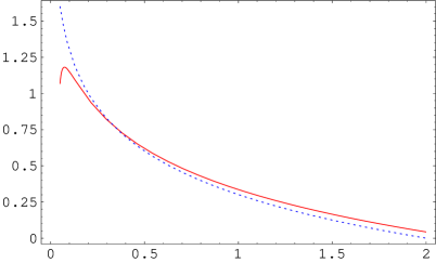
FIG. 3.: The functions $\beta_{0}^{2}(p)$ (continuous line) and $2/p$ (dashed line). The two functions intersect in $p=1/3$, and $\beta_{0}^{2}>2/p$ for $p>1/3$.

Because of the symmetry under time reversal, early time solutions in an expanding universe are the same as late time ones in a contracting universe [43]. Therefore, the solution in the contracting case is never stable: this means that the introduction of a generalized free axion destroys the stability of the single field contracting scaling solution with negative potential ($p<1/3$) studied in [43].

REFERENCES

- [1] G. Veneziano, Phys. Lett. B 265, 287 (1991).
- [2] M. Gasperini and G. Veneziano, Astropart. Phys. 1, 317 (1993) [arXiv:hep-th/9211021].
- [3] J. E. Lidsey, D. Wands and E. J. Copeland, Phys. Rept. 337, 343 (2000) [arXiv:hep-th/9909061].
- [4] M. Gasperini and G. Veneziano, arXiv:hep-th/0207130.
- [5] J. Khoury, B. A. Ovrut, P. J. Steinhardt and N. Turok, Phys. Rev. D 64, 123522 (2001) [arXiv:hep-th/0103239].
- [6] P. Kraus, JHEP 9912, 011 (1999) [arXiv:hep-th/9910149].
- [7] A. Kehagias and E. Kiritsis, JHEP 9911, 022 (1999) [arXiv:hep-th/9910174].
- [8] S. H. Alexander, JHEP 0011, 017 (2000) [arXiv:hep-th/9912037].
- [9] R. Brustein, M. Gasperini, M. Giovannini, V. F. Mukhanov and G. Veneziano, Phys. Rev. D 51, 6744 (1995) [arXiv:hep-th/9501066].
- [10] D. H. Lyth, Phys. Lett. B 524, 1 (2002) [arXiv:hep-ph/0106153].
- [11] R. Brandenberger and F. Finelli, JHEP 0111, 056 (2001) [arXiv:hep-th/0109004].
- [12] J. c. Hwang, Phys. Rev. D 65, 063514 (2002) [arXiv:astro-ph/0109045].
- [13] S. Tsujikawa, Phys. Lett. B 526, 179 (2002) [arXiv:gr-qc/0110124].
- [14] S. Tsujikawa, R. Brandenberger and F. Finelli, arXiv:hep-th/0207228.
- [15] J. Khoury, B. A. Ovrut, P. J. Steinhardt and N. Turok, Phys. Rev. D 66, 046005 (2002) [arXiv:hep-th/0109050].
- [16] R. Durrer and F. Vernizzi, arXiv:hep-ph/0203275.
- [17] E. J. Copeland, R. Easther and D. Wands, Phys. Rev. D 56, 874 (1997) [arXiv:hep-th/9701082].
- [18] S. Rasanen, Nucl. Phys. B 626, 183 (2002) [arXiv:hep-th/0111279].
- [19] R. Kallosh, L. Kofman and A. D. Linde, Phys. Rev. D 64, 123523 (2001) [arXiv:hep-th/0104073].
- [20] V. Bozza, M. Gasperini, M. Giovannini and G. Veneziano, Phys. Lett. B 543, 14 (2002) [arXiv:hep-ph/0206131].
- [21] D. H. Lyth and D. Wands, Phys. Lett. B 524, 5 (2002) [arXiv:hep-ph/0110002].
- [22] S. Mollerach, Phys. Rev. D 42, 313 (1990).
- [23] K. Enqvist and M. S. Sloth, Nucl. Phys. B 626, 395 (2002) [arXiv:hep-ph/0109214].
- [24] T. Moroi and T. Takahashi, Phys. Lett. B 522, 215 (2001) [arXiv:hep-ph/0110096].
- [25] A. Notari and A. Riotto, Nucl. Phys. B 644, 371 (2002).
- [26] F. Finelli, Phys. Lett. B 545, 1 (2002).
- [27] M. Axenides, R. H. Brandenberger and M. S. Turner, Phys. Lett. B 126, 178 (1983).
- [28] C. Gordon, D. Wands, B. A. Bassett and R. Maartens, Phys. Rev. D 63, 023506 (2001) [arXiv:astro-ph/0009131].
- [29] A. L. Berkin and K. I. Maeda, Phys. Rev. D 44, 1691 (1991).
- [30] A. A. Starobinsky, S. Tsujikawa and J. Yokoyama, Nucl. Phys. B 610, 383 (2001) [arXiv:astro-ph/0107555].
- [31] F. Finelli and R. Brandenberger, Phys. Rev. D 65, 103522 (2002) [arXiv:hep-th/0112249].
- [32] V. F. Mukhanov, H. A. Feldman and R. H. Brandenberger, Phys. Rept. 215, 203 (1992).
- [33] J. Garcia-Bellido and D. Wands, Phys. Rev. D 52, 6739 (1995) [arXiv:gr-qc/9506050].
- [34] D. H. Lyth, Phys. Rev. D 31, 1792 (1985).
- [35] V. F. Mukhanov, Sov. Phys. JETP 67, 1297 (1988) [Zh. Eksp. Teor. Fiz. 94N7, 1 (1988)].
- [36] A. L. Berkin, K. Maeda, and J. Yokoyama, Phys. Rev. Lett. 65, 141 (1990).
- [37] E. J. Copeland, J. Gray and A. Lukas, Phys. Rev. D 64, 126003 (2001) [arXiv:hep-th/0106285].
- [38] K. A. Malik and D. Wands, Phys. Rev. D 59, 123501 (1999) [arXiv:astro-ph/9812204].
- [39] F. Finelli and R. Brandenberger, Phys. Rev. D 62, 083502 (2000) [arXiv:hep-ph/0003172].
- [40] M. Parry and R. Easther, Phys. Rev. D 59, 061301 (1999) [arXiv:hep-ph/9809574]; M. Parry and R. Easther, Phys. Rev. D 62, 103503 (2000) [arXiv:hep-ph/9910441]; F. Finelli and S. Khlebnikov, Phys. Lett. B 504, 309 (2001) [arXiv:hep-ph/0009093]; F. Finelli and S. Khlebnikov, Phys. Rev. D 65, 043505 (2002) [arXiv:hep-ph/0107143].
- [41] A. D. Linde and V. Mukhanov, Phys. Rev. D 56, 535 (1997) [arXiv:astro-ph/9610219].
- [42] G. N. Felder, A. Frolov, L. Kofman and A. Linde, Phys. Rev. D 66, 023507 (2002) [arXiv:hep-th/0202017].
- [43] I. P. Heard and D. Wands, arXiv:gr-qc/0206085.
- [44] C. Wetterich, Nucl. Phys. B 302, 668 (1988).
- [45] D. Wands, E. J. Copeland, and A. R. Liddle, Ann. (N.Y.) Acad. Sci. 688, 647 (1993).
- [46] C. Wetterich, Astron. Astrophys. 301, 321 (1995); L. Amendola, Phys. Rev. D 62, 043511 (2000).
- [47] A. R. Liddle, A. Mazumdar, F. E. Schunck, Phys. Rev. D 58, 061301 (1998).
- [48] J. J. Halliwell, Phys. Lett. B 185, 341 (1987).
- [49] E. J. Copeland, J. E. Lidsey, D. Wands, Nucl. Phys. B 506, 407 (1997)