Fireball Models for Flares in AE Aquarii
Abstract
We examine the flaring behaviour of the cataclysmic variable AE Aqr in the context of the ‘magnetic propeller’ model for this system. The flares are thought to arise from collisions between high density regions in the material expelled from the system after interaction with the rapidly rotating magnetosphere of the white dwarf. We calculate the first quantitative models for the flaring and calculate the time-dependent emergent optical spectra from the resulting hot, expanding ball of gas. We compare the results under different assumptions to observations and derive values for the mass, lengthscale and temperature of the material involved in the flare. We see that the fits suggest that the secondary star in this system has Population II composition.
keywords:
accretion, radiative transfer, stars: flares, stars: individual: AE Aqr, novae, cataclysmic variables1 Introduction
AE Aqr is an unusual cataclysmic variable star exhibiting bizarre phenomena that can now be interpreted in the context of a magnetic propeller that throws gas out of the binary system [Wynn, King & Horne 1997]. The magnetic propeller efficiently extracts energy and angular momentum from the white dwarf and transports it via magnetic fields to gas stream material which it ejects from the binary system. Detailed understanding of the magnetic propeller effects may therefore help us to unlock some of the secrets of magnetic viscosity in accretion flows.
In the AE Aqr binary system, a slightly evolved K star [Welsh, Horne & Gomer 1995] that overflows its Roche lobe is locked in a 9.88 hour orbit with a rapidly spinning magnetized white dwarf. Coherent oscillations in optical [Patterson 1979], ultraviolet [Eracleous et al. 1994], and X-ray [Patterson et al. 1980] lightcurves reveal the white dwarf’s 33s spin period. The oscillation has two unequal peaks per spin cycle, consistent with broad hotspots on opposite sides of the white dwarf above and below the equator [Eracleous et al. 1994]. These oscillations are strongest in the ultraviolet, where their spectra show a blue continuum with broad Ly absorption consistent with a white dwarf () atmosphere with [Eracleous et al. 1994]. The simplest interpretation is accretion heating near the poles of a magnetic dipole field tipped almost perpendicular to the rotation axis.
An 11-year study of the optical oscillation period [de Jager 1994] shows that the white dwarf is spinning down at an alarming rate. Something extracts rotational energy from the white dwarf at a rate ie. some 60 times the luminosity of the system. We now believe that to be a magnetic propeller. This model was first proposed by ?) and ?) and expanded upon in ?) with comparison of observed and modelled tomograms. Further work on the flaring region was reported in ?) and ?).
The gas stream emerging from the companion star through the L1 nozzle encounters a rapidly spinning magnetosphere. The rapid spin makes the effective ram pressure so high that only a low-density fringe of material becomes threaded onto field lines. Most of the stream material remains diamagnetic, and is dragged toward co-rotation with the magnetosphere. As this occurs outside the co-rotation radius, this magnetic drag propels material forward, boosting its velocity up to and beyond escape velocity. The material emerges from the magnetosphere and sails out of the binary system. This process efficiently extracts energy and angular momentum from the white dwarf, transferring it via the long-range magnetic field to the stream material, which is expelled from the system. The ejected outflow consists of a broad equatorial fan of material launched over a range of azimuths on the side away from the K star.
The material stripped from the gas stream and threaded by the field lines has a different fate, one which we believe gives rise to the radio and X-ray emission. This material co-rotates with the magnetosphere while accelerating along field lines either toward or away from the white dwarf under the influences of gravity and centrifugal forces. The small fraction of the total mass transfer that leaks below the co-rotation radius at accretes down field lines producing the surface hotspots responsible for the 33s oscillations. Particles outside co-rotation remain trapped long enough to accelerate up to relativistic energies through magnetic pumping, eventually reaching a sufficient energy density to break away from the magnetosphere [Kuijpers et al. 1997]. The resulting ejection of balls of relativistic magnetized plasma is thought to give rise to the flaring radio emission [Bastian, Dulk & Chanmugam 1988a, Bastian, Dulk & Chanmugam 1988b].
This paper addresses the optical and ultraviolet variability seen in AE Aqr. In many studies the lightcurves exhibit dramatic flares, with 1-10 minute rise and fall times [Patterson 1979, van Paradijs, Kraakman & van Amerongen 1989, Bruch 1991, Welsh, Horne & Oke 1993]. The flares seem to come in clusters or avalanches of many super-imposed individual flares separated by quiet intervals of gradually declining line and continuum emission [Eracleous & Horne 1996, Patterson 1979]. These quiet and flaring states typically last a few hours. Power spectra computed from the lightcurves have a power-law form, with larger amplitudes on longer timescales. ?) found that the index in was -1. That is, that the amplitude of the flare or flicker varies inversely as the frequency of its occurence. ?) examined several datasets and found values for in the range –. Such power-law spectra are often associated with physical processes involving self-organized criticality, for example earthquakes, snow or sandpile avalanches [Bak 1996]. Similar red noise power spectra are seen in active galaxies, X-ray binaries, and other cataclysmic variables, and is therefore regarded as characteristic of accreting sources in general. However, flickering in other cataclysmic variables typically has an amplitude of 5-20% [Bruch 1992], contrasting with factors of several in AE Aqr. If the mechanism is the same, then it must be weaker or dramatically diluted in other systems.
The optical and ultraviolet spectra of the AE Aqr flares are not understood at present except in the most general terms. The lines and continua rise and fall together, with little change in the equivalent widths or ratios of the emission lines [Eracleous & Horne 1996]. This suggests that the flares represent changes in the amount of material involved more than changes in physical conditions. The Balmer emission lines decay somewhat more slowly than the optical continuum – perhaps revealing a recombination time delay [Welsh, Horne & Gomer 1998]. Ultraviolet spectra from HST reveal a wide range of lines representing a diverse mix of ionization states and densities. ?) conclude:
“Based on the critical densities of the observed semiforbidden lines we suggest that in a large fraction of the line-emitting gas the density is in the range –. It is likely that denser regions also exist.”
thus setting a lower limit on the density range in the flaring region. Such spectra suggest shocks. The CIV emission is unusually weak, suggesting non-solar abundances. For example, carbon depletion may occur if CNO-processed material is being transferred from the secondary star, which is an evolved star being whittled down by Roche lobe overflow. So far no quantitative fits to the spectra have been achieved either by shock or photo-ionization models. IUE observations by ?) derive an emission measure () from Ly of . UBVRI colour photometry of flares by ?) give colour indices close to those for a blackbody in the –K range with an emitting area .
What mechanism triggers these dramatic optical and ultraviolet flares? Clues come from multi-wavelength co-variability and orbital kinematics. Simultaneous VLA and optical observations show that the radio flux variations occur on similar timescales but are not correlated with the optical and ultraviolet flares, which therefore require a different mechanism [Abada-Simon et al. 1995]. It was proposed that the flares represent modulations of the accretion rate onto the white dwarf, so that they should be correlated with X-ray variability. Some correlation was found, but the correlation is not high. However, HST observations discard this model, because the ultraviolet oscillation amplitude is unmoved by transitions between the quiet and flaring states [Eracleous & Horne 1996]. This disconnects the origins of the oscillations and flares, and the oscillations arise from accretion onto the white dwarf, so the flares must arise elsewhere.
Further clues come from emission line kinematics. The emission line profiles may be roughly described as broad Gaussians with widths km s-1, though they often exhibit kinks and sometimes multiple peaks. Detailed study of the Balmer lines [Welsh, Horne & Gomer 1998] indicates that the new light appearing during a flare can have emission lines shifted from the line centroid and somewhat narrower, km s-1. Individual flares therefore occupy only a subset of the entire emission-line region.
The emission line centroid velocities vary sinusoidally with orbital phase, with semi-amplitudes km s-1 and maximum redshift near phase 0.8 [Welsh, Horne & Gomer 1998]. These unusual orbital kinematics are shared by both ultraviolet and optical emission lines. The implication is that the flares arise from gas moving with a km s-1 velocity vector that rotates with the binary and points away the observer at phase 0.8. This is hard to understand in the standard model of a cataclysmic variable star, though many cataclysmic variables show similar anomalous emission-line kinematics [Thorstensen et al. 1991]. Kepler velocities in an AE Aqr accretion disc would be km s-1 (though we believe no disc to be present.) The gas stream has a similar direction but its velocity is km s-1. A success of the magnetic propeller models is its ability to account for the anomalous emission-line kinematics. The correct velocity amplitude and direction occurs in the exit fan just outside the Roche lobe of the white dwarf. But the question remains of why the flares are ignited here, several hours after the gas slips silently through the magnetosphere.
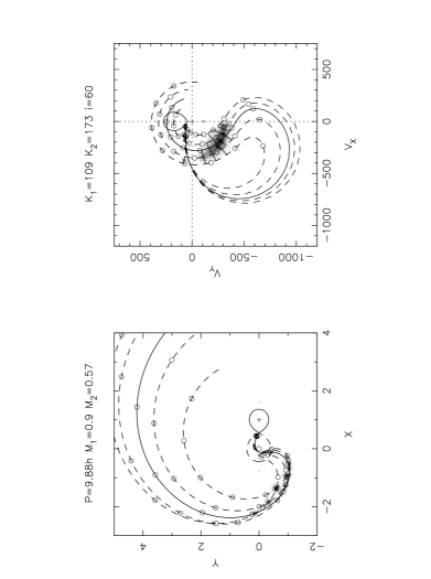
The key insight which solved this puzzle was the realization that the magnetic propeller acts as a blob sorter. More compact, denser, diamagnetic blobs are less affected by magnetic drag. They punch deeper into the magnetosphere and emerge at a larger azimuth with a smaller terminal velocity. These compact blobs can therefore be overtaken by ‘fluffier’ blobs ejected with a larger terminal velocity in the same direction, having left the companion star somewhat later but spent less time in the magnetosphere [Wynn, King & Horne 1997]. The result is a collision between two gas blobs, which can give rise to shocks and flares. Calculations of the trajectories of magnetically propelled diamagnetic blobs with different drag coefficients indicate that they cross in an arc-shaped region of the exit stream, in just the right place to account for the orbital kinematics of the emission lines [Welsh, Horne & Gomer 1998, Horne 1999]. Figure 1 shows how these trajectories map to a locus of points in the lower left quadrant of the Doppler map that is otherwise difficult to populate.
There remains the problem of developing a quantitative understanding of the unusual emission-line spectra of the blobs. We have two aims for this paper: the principle aim is to see if the observed peak optical flare spectrum can be reproduced by conditions appropriate to the aftermath of a collision between blobs. The secondary objective is to develop as far as possible an understanding of the mechanisms by which the observed spectra are formed and evolve. We have approached both goals in the spirit of attempting to find the simplest models that explain the observations.
In section 2 we outline the basic assumptions used in our models. We go on in section 3 to consider the radiative transfer problem and calculate analytic expressions for the behaviour of the optical flare spectra and lightcurves and outline some numerical considerations . In section 4 we present the results of numerical simulations of the flare behaviour, both lightcurves and spectra, and consider further the limits of applicability of our method. We discuss the interpretation of our results in section 5 in terms of the fireball model. Finally we summarise our results in section 6.
2 Fireball Models
2.1 Rough Estimates
We derive rough estimates for the physical parameters associated with the colliding blobs by using the typical rise time and an observed optical flux mJy with a closing velocity for the blobs. We estimate a mass transfer rate
| (1) |
using a distance of 100pc. This compares to a value from the standard evolutionary equation
| (2) |
[Frank, King & Raine 1992]. The mean density of the overflowing gas stream in a CV can be calculated from
| (3) |
where the stream cross-section
| (4) |
has been derived by several authors [Papaloizou & Bath 1975, Meyer & Meyer-Hofmeister 1983, Hameury, King & Lasota 1986, Ritter 1988, Kovetz, Prialnik & Shara 1988, Sarna 1990, Warner 1995]. With a secondary temperature [Skidmore et al. 2002], we have a mean density,
| (5) |
ie.
| (6) |
where is the mean molecular weight appropriate for a fully ionized gas with solar composition. This is consistent with the lower limits from HST uv observations discussed earlier. It must be remembered that this is the mean density in a smooth stream. A stream composed of discrete blobs of material would have range of densities about this value.
We estimate the total mass involved in the collision to be
| (7) |
The typical pre-collision lengthscale of the problem is given by
| (8) |
Following the collision we might expect a somewhat smaller lengthscale eg.. The above density then suggests an emission measure consistent with the above IUE measurements for an optically thick Ly line.
The initial post collision temperature following a strong shock
| (9) |
Finally we have the energy involved in the collision and maximum possible flare energy
| (10) |
A summary of typical values is provided in Table 1.
| Quantity | Value | |
|---|---|---|
| Observed Flux | mJy | |
| Closing Velocity | ||
| Flare Risetime | 300 | s |
| Mass Transfer Rate | ||
| Fireball Mass | kg | |
| Pre-Collision Lengthscale | m | |
| Initial Temperature | K | |
| Total Energy | J | |
| Typical Density | ||
| Number Density | ||
| Column Density | ||
2.2 Initial Conditions
We envision an expanding fireball emerging from the aftermath of a collision between two masses . In the centre of mass frame, these masses approach with initial velocities satisfying . The initial kinetic energy in the centre of mass frame is
| (11) |
where is the (frame-independent) relative velocity and is the mass ratio. Note that for a given and a range of energies is possible, ranging from zero for very extreme mass ratios up to a maximum of for equal masses.
As the collision progresses, some of the energy is converted to thermal energy through dissipation in shocks. The initial dissipative phase lasts a short time
| (12) |
The ratio of energy per mass sets the initial temperature and sound speed through
| (13) |
where a specific heat ratio is appropriate for fully ionized atomic gas. For km s-1, , so that the initial ball of hot gas is atomic and completely ionized.
Since , sound waves have time to cross the initial fireball during the collision time , and we therefore expect a roughly uniform temperature profile inside .
2.3 Expansion
With nothing to hold it back, the hot ball of gas expands at the initial sound speed, launching a fireball. We adopt a uniform, spherically symmetric, Hubble-like expansion , in which the Eulerian radial coordinate of a gas element is given in terms of its initial position and time by
| (14) |
This defines an expansion factor which we can use as a dimensionless time parameter. The ‘Hubble’ constant is set by the initial conditions .
Uniform free expansion is a suitable approximation because the flow becomes supersonic as it expands and cools. If we can determine parameters at some time ie. for the lengthscale (), temperature () and mass () we can derive the time evolution as follows. We adopt a Gaussian density profile
| (15) |
where
| (16) |
is the initial central density and
| (17) |
is a dimensionless radius coordinate, the radius scaled to the lengthscale .
Although this Gaussian density profile is only a guess, it is motivated by the Gaussian shapes of observed velocity profiles, and by the thought that the initial thermal velocity distribution in the hot gas will map into the density profile of the expanding fireball because the fast particles travel farther than slow ones.
2.4 Cooling
We consider three cooling schemes: adiabatic, isothermal and radiative. The adiabatic fireball cools purely as a result of its expansion and corresponds to a situation where the radiative and recombination cooling rates are negligible. In contrast, the isothermal model maintains a fixed temperature throughout its evolution. A truly isothermal fireball would require a finely balanced energy source to counteract the expansion cooling. However, it may an appropriate approximation to a situation where a photospheric region dominates the emission and presents a fixed effective temperature to the observer as a result of the stong dependence of opacity on temperature. The radiative models cool adiabatically throughout and as a result of radiation from a thin zone near the photosphere which we model by immediately dropping the temperature to at this surface.
2.4.1 Adiabatic Cooling
During adiabatic expansion, and . If we consider the evolution of a given gas element then, with , the temperature decreases with time as
| (18) |
We see that an initially uniform temperature distribution remains uniform and so, for this case, we can write, more simply,
| (19) |
With for a monatomic gas, , and so the sound speed . The sound crossing time . The fireball becomes almost immediately supersonic. We can derive the behaviour of the sonic point from the definition that it is the position where the expansion rate matches the sound speed. Thus,
| (20) |
Assuming a uniform temperature profile and , this gives
| (21) |
Hence, we can see that the sonic point remains fixed in space at . The initial density structure emerging through the sonic surface at radius is subsequently ‘frozen in’ by the rapid expansion.
2.4.2 Radiative Cooling Timescales
The time required for the fireball to radiate away its internal energy depends crucially on the temperature of the photosphere (assuming that the fireball is optically thick). For a uniform temperature distribution the timescale is very short:
| (22) | |||||
| (23) |
We would thus expect the region from which the radiation escapes to cool rapidly until the region becomes optically thin and the cooling efficiency drops.
If the photospheric temperature is significantly cooler than the optically thick region, the radiative timescale
| (25) |
can become comparable to the evolutionary timescale of the fireball.
2.4.3 Radiative Cooling Front
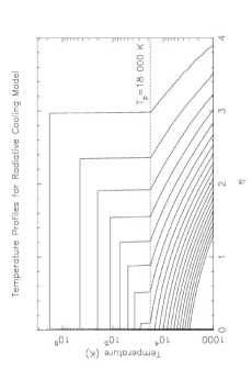
Following the exact behaviour of radiative cooling and heating is a complex process requiring us to follow the behaviour of the internal radiation field of the fireball through the optically thick to optically thin transition. Such detailed modelling is beyond the scope of the initial investigations presented here. We note that studies of cooling from optically thin plasmas [Lynden-Bell & Tout 2001, Dalgarno & McCray 1972] show that there is a significant reduction in efficiency due to hydrogen recombination and the consequent loss of free electrons below approximately K. Since the photosphere is the region where the optical depth for escaping radiation is unity, this suggests that the photosphere may adopt a roughly constant effective temperature . The relatively dense material in the fireball will be able to cool rapidly down to this temperature before the cooling rate stalls. We approximate a radiatively cooling fireball by maintaining a hot core region which cools adiabatically as it expands. Once gas elements cross the boundary to this region, we assume them to cool immediately to the effective temperature of the photosphere and thereafter adiabatically. We derive the radius of the photospheric surface below, using the blackbody luminosity and the thermal energy of the central region.
To find the photospheric radius in our radiative model we calculate the total thermal energy in a sphere of radius
| (26) | |||||
| (27) |
Hence, differentiating,
| (28) |
Radiative cooling at fixed effective temperature gives
| (29) |
and so, using
| (30) |
we have the differential equation for the core radius as a function of time
| (31) |
where
| (32) |
We solve equation (31) numerically and plot the behaviour for typical parameters in Fig. 2. We see how, in the Lagrangian coordinate , the boundary migrates inward continually. In Eulerian coordinates, plotted in Fig. 3, the boundary is initially advected outwards with the flow. When the inward migration exceeds the expansion rate, the photosphere turns around and begins to collapse. In both plots the initial conditions for have relatively little impact on the behaviour at late times. Models with initially are indistinguishable as they rapidly converge on the same curve. Lower initial values for also converge, albeit more slowly, on the same evolution.


We plot the temperature profiles at different times for the radiative model in Fig. 4. The profiles show how the material outside the core region cools very rapidly with distance away from the boundary. As a result, the shell of material with significant temperature outside the core is very thin. For computational convenience we set a minimum temperature for any of the gas at K.
2.5 Ionization Structure
In the LTE approximation, the density and temperature determine the ionization state of the gas at each point in space and time through the solution of a network of Saha equations. Atomic level populations are similarly determined through Boltzmann factors and partition functions. For purely adiabatic cooling, the temperature retains its initial uniform spatial profile, but decreases with time. The LTE ionization is therefore higher in the outer low-density regions which also move fastest. Thus in the LTE model high ionization emission lines are predicted to have broader velocity profiles.
Once we have determined the evolution of and with time, we can follow the evolution of the ionization structure and determine the boundaries between different ionization states of various species. We do so for hydrogen and helium for an adiabatic Population II model in Fig. 5 and for carbon in Fig. 6. We plot boundaries for the same species for an isothermal Population II model in Figs. 7 and 8. In both cases we use , and .


At a given time, the various ionic species form onion layers of increasing ionization on moving outwards from the fireball centre. The different temperature evolutions significantly alter the ionization evolution. The adiabatic temperature evolution causes the ionization states to alter rapidly throughout the structures when the fireball passes the appropriate critical temperatures. The isothermal evolutions show the gentler dependance of ionization on density. The spatial structure remains roughly constant and only evolves slowly as the density drops.
2.6 Ionization Freezing
For the initial models presented here we have assumed that the ionization structure produced at any point is given by LTE; an assumption we justify in Appendix A. In reality, of course, once the LTE boundary is crossed, the ionization will drop as the net recombination rate gradually ekes away at the ions and we make a transition towards coronal equilibrium. However, since we know the time-evolution of density and temperature for any region outside of the LTE limiting radius, we can derive the time and conditions when it crossed this LTE boundary. In principle then, we can follow the non-LTE evolution of the gas through this outer region and beyond the ion-electron equilibrium radius to the non-equilibrium ionization states present in the outer fringe.
In a purely LTE fireball we expect high ionization states to occur in the outer regions as a result of the lower density. With the more detailed prescription above, the higher ionization would result from the higher temperature of the fireball when the region in question crossed the LTE boundary. In practice, we expect that this correction may have little effect on the optical spectra because the emission is dominated by the higher density inner regions of the fireball. This effect may well become important, however, when we come to consider the ultraviolet spectra where high ionization lines are present; and which we hope to consider in a future paper. An alternative explanation for the ultraviolet behaviour may be that there is a hot, low density outer fringe to the fireballs. These conditions may occur in regions that have always been optically thin and inefficient at cooling radiatively. These lines may then arise from a transition region similar to that between the solar chromosphere and corona.
3 Radiative Transfer
The radiative transfer equation has a formal solution
| (33) |
where is the intensity of the emerging radiation, is the source function, and is the optical depth measured along the line of sight from the observer. This integral sums contributions to the radiation intensity, attenuating each by the factor because it has to pass through optical depth to reach the observer.
Since we have assumed LTE, the source function is the Planck function, and opacities both for lines and continuum are also known once the velocity, temperature, and density profiles and element abundances are specified. The integral can therefore be evaluated numerically, either in this form or more quickly by using Sobolev resonant surface approximations.
The above line integral gives the intensity for lines of sight with different impact parameters . We let measure distance from the fireball centre toward the observer, and the distance perpendicular to the line of sight. The fireball flux, obtained by summing intensities weighted by the solid angles of annuli on the sky, is then
| (34) |
where is the source distance.
3.1 Continuum Lightcurves and Spectra
In a forthcoming paper (Pearson, Horne & Skidmore, in prep.) we will consider generic analytic models for fireball behaviour applicable to a variety of systems. We use the general opacity given in equation (54). We quote here an approximation to the lightcurve behaviour being the sum of optically thick and optically thin contributions:
| (35) |
where
| (36) | |||||
| (37) | |||||
| (38) | |||||
| (39) | |||||
| (40) | |||||
| (43) |
Here is the time that the fireball first becomes optically thin through its centre and is the current optical depth through the fireball centre.
The peak flux occurs when
| (44) |
which occurs at a time
| (45) |
We note that equations (37) and (45) predict that the peak flux will occur at different times for different wavelengths. In principle we could use this as a test for the effective . However, in practice, both the assumptions in our treatment and the necessary accuracy of observations, might make it difficult to detect the difference between for an isothermal fireball and for adiabatic cooling. In contrast, the late time behaviour is predicted to have a more significant dependance on
| (46) |
Coverage of a full flare may well make the or difference discernable.
The total flux at several wavelengths and the optically thick contribution at Å are plotted in Figs. 9 and 10 for 2 sets of physical conditions, using Population I composition and a distance of . The corresponding spectral distributions for one of the parameter sets are plotted in Figs. 11 and 12. We would expect the early and late time behaviours to be accurately represented by this analysis, but the detailed behaviour when both free-free and bound-free opacity sources are important is less exact.


The lightcurves for the isothermal models show a rise to the peak value before turning over and undergoing a slower decline. The predicted fluxes are very similar to observed fireballs and morphologically the similarity to observations is remarkable. It is also clear that the peak flux is independent of our choice of fiducial size. We can see how the combination of the overall spectral slope and the large Balmer jump at early times leads to the Å curve exceeding that for Å. As ionization occurs due to the decreasing density, bound-free opacity becomes less important and the Balmer jump declines. The Å curve then drops below the Å and behaves similarly to the other curves in the family. The size of our Balmer jump, however, is still smaller than that observed suggesting that we may need to improve the treatment of opacity across this region.
The adiabatic lightcurves, however, show only a decline from a large initial flux. We would expect the evolution of the optically thick region here to be similar to that of the radiative core photosphere ie. it would be initially advected outward with the flow before eventually turning over and collapsing back to zero size. The emitted flux, however, does not follow this scheme as the fireball is extremely hot at early times and the evolution of temperature and the blackbody intensity dominates the lightcurve evolution. The spectra in this case only begin to show a Balmer jump late on in the evolution once the fireball has cooled enough for significant recombination to have taken place.
3.2 Fireball Tomography
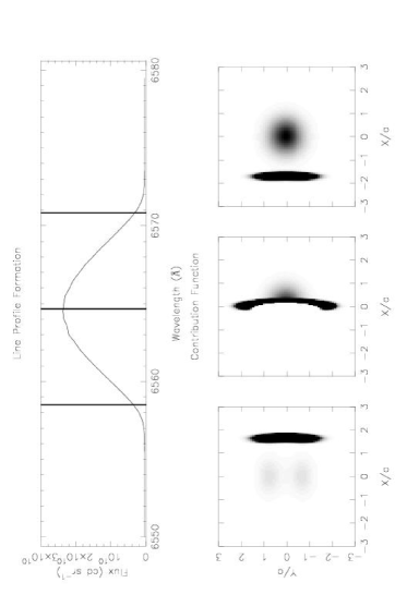
For our spherical expansion the component of velocity along the line of sight is proportional to the distance from the centre towards the observer, ie. . As a result, each velocity in the emission line profile originates from a unique surface perpendicular to the line of sight. This is illustrated in Fig. 13, which shows a side view of the fireball with the contribution to the flux at 3 different velocities in the H profile. On the blue side of line centre, the resonant surface, approximately perpendicular to the line of sight, is on the near side of the fireball. The fireball is optically thick through its centre but sufficiently transparent at larger impact parameters so that small continuum contributions to the flux are made from a peanut shaped region along the -axis about the origin.
The resonant surface at the line centre passes through the centre of the fireball. There is a continuum contribution from the rising density in front of the resonant plane around the origin and then a line contribution from the resonant position. The larger optical depth through the centre compared to larger impact parameters gives rise to the curved shape. The contribution from the back of the resonant region through the line centre is unable to escape to the observer through the overlying material giving rise to the distorted shape.
The flux on the red side of the line shows the two contributing regions more clearly. A continuum contribution with the density peak and then another peak at the resonant position.
Such fireball tomography may allow us, in future, to probe the structure of a fireball using high-resolution spectra. For example, in Fig. 13, the Gaussian velocity profile arises from the assumed Gaussian density profile in equation (15). A different density profile would change the shape of the line profile.
3.3 Numerical Considerations
Our numerical integrations of equation (33) were carried out at appropriate wavelength intervals to resolve the emission line profiles and with spatial steps to reflect the variations in the density and ionization structures. For conservative parameters and , the thermal line width is . Opacity information was therefore generated and stored at wavelength and spatial intervals of and respectively. When generating the full spectra, intensities were calculated every , giving a velocity resolution of at . The integration was carried out with spatial steps that were calculated to be either or whichever was shorter.
In general the opacity at any position in the fireball consisted of both continuum and line contributions. Continuum opacities were generally calculated using the methods of ?) with the exception of H- bound-free [Geltman 1962] and free-free [Stilley & Callaway 1970], He- [McDowell, Williamson & Myerscough 1966] and HeI bound-free [Huang 1948]. Line opacities used oscillator strengths and energy level information downloaded from the NIST atomic database111 http://physics.nist.gov/cgi-bin/AtData/main_asd.
We aim, in the longer term, to speed-up our code by using a Sobolev method, ie. use the fact that velocity is a monotonically increasing function of position, to find the resonant point in the fireball at each wavelength for a given line. We might also achieve time savings by identifying regions where no lines make significant contributions to the flux. These methods would enable us to use coarser grids or precalculated tables when appropriate. This would simplify the integration scheme and possibly allow us to fit both the emission lines and continuum simultaneously with an amoeba code.
4 Comparison with Observations
4.1 Observed Flare in AE Aqr
To test our fireball model, we aimed to reproduce the observations reported in ?) of high time-resolution optical spectra of an AE Aqr flare taken with the Keck telescope. The lightcurve formed from these data is plotted in Fig. 14. Although the dataset only lasts around 13 minutes it shows the end of one flare and beginning of another. The major features of the flaring observed in the system are apparent in the lightcurve.

We extracted the spectrum of the second flare by subtracting the quiescent spectrum (Q) from the spectrum at the top of the new flare (P). The resultant optical spectrum is plotted in the bottom panel of Fig. 15. Gaussian profiles fitted to several lines gave the parameters in Table 2. Assuming the instrumental profile is also Gaussian, we remove the formal instrumental blurring ( FWHM) to estimate the expansion velocity.
These widths suggest a velocity dispersion of around . Ascribing this to the velocity at of the density distribution gives a velocity of at . Such a high velocity is larger than the expected from Doppler tomography [Welsh, Horne & Gomer 1998] and may indicate that an additional, unknown source of blurring is present. Examination of the arc line spectra support this suggestion. Since these were taken by flooding a large aperture with light it is not possible to accurately measure the instrumental effect from these lines, but the line edges do suggest that the instrumental blurring is significantly larger than the formally derived value.
| Line | Fitted FWHM | Deconvolved FWHM |
|---|---|---|
| (km ) | (km ) | |
| H | ||
| HeI 5876 | ||
| HeI 4922 | ||
| H | ||
| H | ||
| H | ||
| H | ||
| CaH |
4.2 Spectral Fit at Peak of Flare
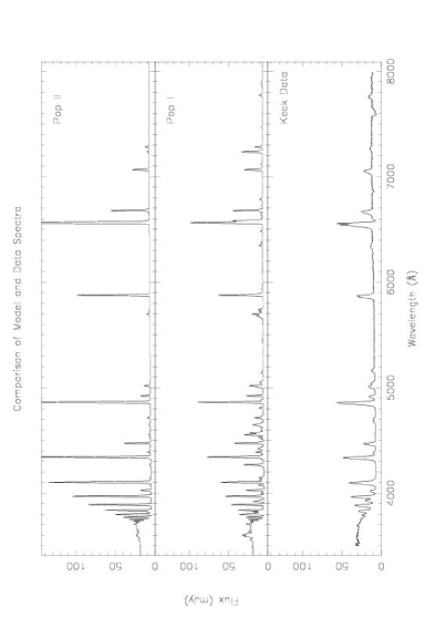
To estimate the fireball parameters , and from the observed optical spectra we began with consideration of the continuum flux. We considered both Population I and Population II abundances. Population I abundances were set using the solar abundances presented by ?). For population II composition, we decreased from 0.085 to 0.028 the ratio of the helium to hydrogen number densities and reduced the ratio for each metal abundance to 5% of solar [Bowers & Deeming 1984]. In either case we used an amoeba algorithm [Press et al. 1986] to optimize the fit by reducing to a minimum for the 6 measured continuum fluxes in Table 3. The best fit parameters , and and related secondary quantities are listed in Table 4.
Using Population I composition, we derived parameters for the fireball at its peak of kg, m and K. Such a mass represents approximately 100 s of the L1 mass transfer rate derived from equation (2). Fig. 15 and Table 3 show that these parameters provide a reasonably good fit to the observed Paschen continuum and Balmer Jump.
Population II composition produced best fit parameters of kg, m, K.
Both compositions arrive at a model fit with remarkably similar calculated fluxes which have a slightly steeper slope to the Paschen continuum than the observations. The fits also produce a large Balmer jump but appears to have difficulty in creating one quite as strong as that observed. A change in the 3rd significant figure of one of the fit parameters generally leads to a similar change in the calculated fluxes. Both sets of parameters have similar temperatures but the Population II models require roughly a factor 2 increase in mass and lengthscale equivalent to a factor 4 decrease in density. The central densities implied by both sets of parameters are consistent with the typical values for the gas stream derived in section 2.1 and with the temperature range and emitting area of ?).
| Range | Central Wavelength | Mean Flux | Pop I Fluxes | Pop II Fluxes |
|---|---|---|---|---|
| (Å) | (Å) | (mJy) | (mJy) | (mJy) |
| 3602–3630 | 3616 | 27.3 | 28.3 | |
| 4150–4250 | 4200 | 6.65 | 6.64 | |
| 4520–4640 | 4580 | 7.52 | 7.49 | |
| 4735–4780 | 4758 | 7.89 | 7.85 | |
| 5400–5600 | 5500 | 9.13 | 9.13 | |
| 5600–5775 | 5688 | 9.37 | 9.39 |
| Quantity | Pop I | Pop II |
|---|---|---|
| (K) | ||
| (s) | ||
Fig. 16 shows the area around the H line produced with the Population I best fit parameters and with zero and modest expansion velocities, showing the intrinsic thermal resolution of the lines and the Doppler blurring due to the expansion before instrumental effects are added. Even with a relatively modest fiducial expansion velocity of we can see that many of the weaker lines are blurred into obscurity simply by the Doppler effect. The H line at Å appears to be optically thick since its peak flux decreases only slightly as the line width increases. In contrast, the ArII line at Å decreases greatly with Doppler broadening and forms a blend with the weaker blueward NII line indicating that it is optically thin.

In Fig. 17 we plot the observed data around H alongside Population I models generated with various expansion velocities. We consider the H region because the observed H line shows a complex structure. We blurred the model spectra with a Gaussian of FWHM and assumed a distance of pc [Friedjung 1997]. To match the peak flux of H requires an expansion velocity of at . The HeI line at Å suggests an expansion velocity of . The model lines are clearly narrower than the data. Considering this and the possibility of additional, unidentified blurring suggests that a more reliable estimate might be the integrated line flux. In this case, the H and HeI line suggest expansion velocities of and respectively at . Consequently, we adopt an expansion velocity at of for the simulations.

The optical spectra produced with both compositions are compared to the observed mean spectrum at the flare peak in Fig. 15. We see that the parameters, derived from the peak continuum fluxes alone, allow us to derive optical spectra with integrated line fluxes and ratios comparable to the observations. Both models have line widths narrower than the observations, and hence peak line fluxes greater than those observed, which may result from additional unidentified instrumental blurring. The Population I models show the flat Balmer decrement of saturated Balmer lines apparent in the data. Comparing the lines that are present, however, particularly in the Å range, the Population II model appears to produce a much better fit: suppressing the metal lines which do not appear in the observed spectra. Specifically, we note that SiIII, CII, the SiIII blend, OII, the SiI, SiIII and ArII blend and CII are present in the Population I models but are not present or are far weaker in the data. Only the weak CII, CII, the SiII blend and the OI blend are not reproduced by the Population II results.
4.3 Lightcurves and Spectral Evolution
The timescale for the evolution of the fireball implied by the observed lightcurve can be reproduced by the parameters derived solely from fitting to the peak spectrum. The evolutionary timescale is approximately s and s for Population I and II parameters respectively. The encouraging result that these values are similar to the observed timescale suggests that our fireball models are on the right track.
We thus consider the time evolution of the fireball models in more detail. Figs. 18 and 19, for Population I and Population II abundances respectively, present the lightcurves and spectral evolution derived under the three assumptions we consider for the thermal history of the fireball: adiabatic, isothermal, and radiative. In each case, the model fireball is constrained to evolve through the state we found from the fit to the observations at the peak of the flare. This moment is assigned to and hence our assignment of subscripts for the fitted parameters above.
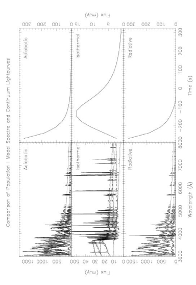
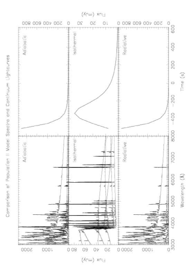
The isothermal models produces a lightcurve that rises and falls, as observed. Moreover, the peak in this lightcurve is in fact reasonably close to the time when the spectrum matches the spectrum observed at the peak of the flare. The isothermal fireball spectra, both on the rise and on the fall of the flare, exhibit strong Balmer emission lines and a Balmer jump in emission. Thus the isothermal fireball model provides a good fit not only to the peak spectrum but also to the time evolution of the AE Aqr flare.
The adiabatic and radiative models both fail to reproduce the observed lightcurve or spectra. The adiabatic model matches the observed spectrum at one time, but is too hot at early times and too cool at late times. As a result the lightcurve declines monotonically from early times rather than rising to a peak and then falling, and the spectra have lines that do not match the observed spectra. This disappointing performance is perhaps not too surprising, since the temperature in this model falls through a wide range while the observations suggest that the temperature is always around K.
For the adiabatic fireball, equation (13) implies that the expansion rate is a measure of the initial temperature. Hence, for an adiabatic fireball we can derive its age from the time taken to cool to the fitted temperature. For the Population I parameters, gives an initial temperature of , an age of and hence from (14) an initial lengthscale of . The Population II parameters give an age of and initial lengthscale of . We note, however, that the lightcurve for the adiabatic fireballs do not show the rise to a peak for the same reason as the theoretical curves in section 3.1. To explain the rise phase of the observed lightcurve we must interpret it as resulting from the collision of the initial gas blobs. Under this assumption, we can estimate the age and initial size independently, for the adiabitic evolution, directly from the data; knowing the rise time of the flare and the typical closing velocities:
| (47) | |||||
| (48) |
The radiative model looks roughly the same as the adiabatic model. This occurs because the cooling front (as shown in Fig. 4) occurs well outside the photosphere. We therefore “see” into the adiabatically-cooling core. This is not consistent with our assumption that the rapid cooling occurs near the photosphere as a result of the opacity drop there and suggests that a more sophisticated approach involving heating of the gas by emergent photons may be required for an accurate treatment of such a model.
5 Discussion
The spectra produced with Population II composition reproduce the optical observations well. The fitted parameters are consistent with both the expected conditions in the mass transfer stream and with the lower limits on the density implied by the uv observations. The presence of high ionization and semi-forbidden lines in the uv data can be understood qualitatively in terms of their formation in the low density outer fringes of the fireball and the wide variety of ionization states by the wide range of densities in the expanding fireball structure. For , and Population II parameters, the density of , important for the uv semi-forbidden lines, occurs at . From Fig. 22 we see that this lies outside the limit for LTE behaviour. Quantitative fits for the fringe and uv behaviour, therefore, remain to be addressed in the non-LTE regime extension to this work.
Parameters implying a lower overall density would result in an optically thinner fireball and spectrum. The Balmer decrement would increase as would the equivalent widths of the optically thick Balmer lines as the continuum dropped away from the blackbody envelope. Continued decrease would result in the lines eventually becoming optically thin and losing the characteristically consistent strengths present when they are all saturated.
The behaviour of the lightcurve for an isothermal model, like its theoretical counterpart is much more similar to the observed lightcurve than the other models giving a peak close to the observed time without the need to invoke the collision process. Clearly though, an expanding gas ball would be expected to cool both from radiative and adiabatic expansion effects.
The radiative model shows very similar behaviour to the adiabatic models. The thin shell of cooling material at around does not provide sufficient opacity to mimic the isothermal behaviour and the adiabatic core is still visible to the outside observer. This effect appears to be insensitive to the exact choice of temperature we assign to material emerging from the central region.
We noted in section 2.6 that an accurate picture of the ionization would need to follow the LTE to non-LTE ionization transition. However, even considering only the early evolution of the fireballs, the isothermal lightcurve and spectral behaviour is stiller closer to the observations than the adiabatic.
In short, we find that isothermal fireballs reproduce the observations rather well, whereas adiabatically cooling fireballs fail miserably! How can the expanding gas ball present a nearly constant temperature at its surface?
5.1 Thermostat
We offer two possible mechanisms which may operate to maintain the apparent fireball temperature in the – region. The first relies on the fact that both free-free and bound-free opacity decrease with temperature and thus opacity peaks just above the temperature at which hydrogen begins to recombine. In the model where a core region is cooling through radiation from its surface, we can envision a situation where the material just outside the core has reached this high opacity regime and is absorbing significant amounts of energy from the core’s radiation field. This would help to counteract the effect of adiabatic cooling and may maintain an effectively isothermal blanket around the core. If the temperature in the blanket were to rise, the opacity would decrease, more energy would escape and the blanket would cool again. Similarly, until recombination, cooling would result in higher opacity and therefore greater heating of the blanket region. For such a thermostatic mechanism to work, the optical depth through the blanket region would need to be high which would be consistent with it being the photosphere as seen by an outside observer. Realistic simulations of such a model would require a detailed treatment of the radiation field and its heating effect using a more sophisticated method than the one we have employed here.
5.2 External Photoionization
Alternatively the ionization of the fireball might be held at a temperature typical of the – range through photoionization by the white dwarf. In Fig. 20 we plot the hydrogen ionization and recombination rates as a function of temperature for a typical electron number density using additional routines for photoionization from Verner et al. (1996) and collisional ionization by Verner using the results of Voronov (1997). We calculate a conservative overestimate for the self-photoionization of the fireball assuming the sky is half filled by blackbody radiation at the given fireball temperature. Also shown is the photoionization due to a blackbody with the same radius and distance as the white dwarf. The general white dwarf temperature is uncertain but, as mentioned earlier, there is evidence to suggest that the hot spots have a temperature of around . We can see that the flux from the white dwarf overtakes that from the fireball itself as the dominant ionization mechanism at . We have assumed a typical distance from the white dwarf for the fireball equal to that of the L1 point from the white dwarf (although in a different direction). The recombination rates for this plot have been calculated assuming is a constant and so for temperatures below about are conservative overestimates of the LTE recombination rate that will occur in our fireball. In spite of this, the white dwarf photoionization at comfortably exceeds the recombination rates down to at least and, hence, we would expect the fireball to remain almost completely ionized in this case. This suggests that the white dwarf radiation field may be the cause of the fireball appearing isothermal when we consider the lightcurve behaviour and consistent line strengths and ratios.
Ionization by an external black body at a different temperature will clearly cause our fireball to no longer be in LTE and require a non-LTE model to follow the fireball behaviour. However, we can anticipate the results of a full non-LTE treatment as follows. Writing the total ionization rate per atom per second from all processes as and similarly the total recombination rate as , we have the simple equilibrium condition
| (49) |
Hence the ionization fraction is given by
| (50) |
We calculate the evolutions of the boundary between HI and HII dominated regions for a pure hydrogen fireball using , and . Since in this simplified case , we can easily iterate to produce self-consistent ionization profiles in cases where b contains contributions from ordinary atomic processes and also an additional contribution from white dwarf photoionization. We plot the evolutions in Fig. 21 for no white dwarf photoionization and with rates appropriate to photoionization from a white dwarf at and . We see that the white dwarf can have a significant effect on the ionization structure of the fireball and keep large parts of it in an ionized state.


6 Summary
We have shown for AE Aqr how the observed flare spectrum and evolution is reproducible with an isothermal fireball at K with Population II abundances but not when adiabatic cooling is incorporated. We suspect that the cause of the apparently isothermal nature is a combination of two mechanisms. First, a nearly isothermal photosphere which is self-regulated by the temperature dependance of the continuum opacity and the hydrogen recombination front and second, particularly at late times, by the ionizing effect of the white dwarf radiation field.
The observed photosphere in the isothermal models is initially advected outward with the flow before the decreasing density causes the opacity to drop and the photosphere to shrink to zero size. This gives rise to a lightcurve that rises and then falls. Emission lines and edges arise because the photospheric radius is larger at wavelengths with higher opacity. Surfaces of constant Doppler shift are perpendicular to the line of sight and thus Gaussian density profiles give rise to Gaussian velocity profiles.
Direct application of our LTE fitting method to the uv region would not reproduce the observed spectra with their variety of ionization states and semi-forbidden and permitted lines. We have outlined techniques and possible improvements to the model that will increase our understanding further and enable us to take the work into the uv. More detailed modelling of the ionization and recombination processes is suggested that also incorporates the heating effects of both the white dwarf’s and the fireballs own photon fields. The self-consistent solution to these rate equations will extend the treatment to the non-LTE regimes discussed in Section 5 and Appendix A. These modifications may in turn have consequences for the predicted optical spectra.
Improved modelling of these fireballs offers us the chance to probe the chemical composition of the secondary star in AE Aqr. Normally this is difficult because the spectrum of the relatively dim secondary star is contaminated by light from other components in the system. We expect that the fireball models will be applicable more generally to the flickering observed in most CV systems.
Acknowledgements
We would like to thank Gary Ferland and Kirk Korista for informative discussions regarding atomic ionization and recombination processes and the routines for calculating them. We are grateful to the anonymous referee and editor for helpful comments that improved the presentation of this paper.
References
- [Abada-Simon et al. 1995] Abada-Simon, M., Bastian, T. S., Horne, K. D., Robinson, E. L., Bookbinder, J. A., 1995, in Buckley, D. A. H., Warner, B., eds., Proc. Cape Workshop on Magnetic Cataclysmic Variables, ASP Conf. Series, 355
- [Arnaud & Raymond 1992] Arnaud, M., Raymond, J., 1992, ApJ, 398, 394
- [Bak 1996] Bak, P., 1996, How nature works: the science of self-organized criticality, Copernicus, New York
- [Bastian, Dulk & Chanmugam 1988a] Bastian, T. S., Dulk, G. A., Chanmugam, G. 1988, ApJ, 324, 431
- [Bastian, Dulk & Chanmugam 1988b] Bastian, T. S., Dulk, G. A., Chanmugam, G. 1988, ApJ, 330, 518
- [Beskrovnaya et al. 1996] Beskrovnaya N., Ikhsanov N., Bruch A., Shakhovskoy N., 1996, A&A, 307, 840
- [Bowers & Deeming 1984] Bowers, R. L., Deeming, T., 1984, Astrophysics I Stars, Jones and Bartlett, Boston
- [Bruch 1991] Bruch A., 1991, A&A, 251, 59
- [Bruch 1992] Bruch, A., 1992, A&A, 266, 237
- [Bruch & Grutter 1997] Bruch A., Gruuter M., 1997, Act Ast, 47, 307
- [Cota 1987] Cota, S. A., 1987, Ph.D. Thesis, Ohio State Univ.
- [Dalgarno & McCray 1972] Dalgarno, A., McCray, R. A., 1972, ARA&A, 10, 375
- [Däppen 2000] Däppen, W., 2000, in Cox, A. N., Allen’s Astrophysical Quantities, Chapter 3, Springer-Verlag, New York
- [de Jager 1994] de Jager, O. C., Meintjes, P. J., O’Donoghue, D., Robinson, E. L., 1994, MNRAS, 267, 577
- [Elsworth & James 1982] Elsworth, Y. P., James, J. F., 1982, MNRAS, 198, 889
- [Eracleous et al. 1994] Eracleous, M., Horne, K. D., Robinson, E. L., Zhang, E.-H., Marsh, T. R., Wood, J. H., 1994, ApJ, 433, 313
- [Eracleous & Horne 1996] Eracleous, M., Horne, K. D., 1996, ApJ, 471, 427
- [Frank, King & Raine 1992] Frank, J., King, A. R., Raine, D. J., 1992, Accretion Power in Astrophysics, Cambridge Univ. Press
- [Friedjung 1997] Friedjung, M., 1997, NewA, 2, 319
- [Geltman 1962] Geltman, S., 1962, ApJ, 136, 935
- [Glasco & Zirin 1964] Glasco, H. P., Zirin, H., 1964, ApJS, 9, 193
- [Goldston & Rutherford 1995] Goldston, R. J., Rutherford, P. H., 1995, Introduction to Plasma Physics, Bristol, IOP Publishing
- [Gray 1976] Gray, D. F., 1976, Observations and Analysis of Stellar Photospheres, New York, Wiley
- [Horne 1999] Horne, K. D., 1999, in Hellier, K., Mukai, K., eds, Annapolis Workshop on Magnetic Cataclymic Variables, ASP Conf. Series, 157, 357
- [Huang 1948] Huang, S., 1948, ApJ, 108, 354
- [Hameury, King & Lasota 1986] Hameury, J. M., King, A. R., Lasota, J.-P., 1986, A&A, 162, 71
- [Jameson, King & Sherrington 1980] Jameson, R. F., King, A. R., Sherrington, M. R., 1980, MNRAS, 191, 559
- [Kingdon & Ferland 1996] Kingdon, J. B., Ferland, G. H., 1996, ApJS, 106, 205
- [Kovetz, Prialnik & Shara 1988] Kovetz, A., Prialnik, D., Shara, M. M., 1988, ApJ, 325, 828
- [Kuijpers et al. 1997] Kuijpers, J., Fletcher, L., Abada-Simon, M., Horne, K. D., Raadu, M. A., Ramsay, G., Steeghs, D., 1997, A&A, 322, 242
- [Landini & Monsignori Fossi 1990] Landini, M., Monsignori Fossi, B. C., 1990, A&AS, 82, 229
- [Landini & Monsignori Fossi 1991] Landini, M., Monsignori Fossi, B. C., 1991, A&AS, 91, 183
- [Lynden-Bell & Tout 2001] Lynden-Bell, D., Tout, C., 2001, ApJ, 558, 1
- [McDowell, Williamson & Myerscough 1966] McDowell, M. R. C., Williamson, J. H., Myerscough, V. P., 1966, ApJ, 144, 827
- [Mazzotta et. al. 1998] Mazzotta, P., Mazzitelli, G., Colafrancesco, S., Vittorio, N., 1998, A&AS, 133, 403
- [Meyer & Meyer-Hofmeister 1983] Meyer, F., Meyer-Hofmeister, E., 1983, A&A, 121, 29
- [Papaloizou & Bath 1975] Papaloizu, J. C. B, Bath, G. T., 1975, MNRAS, 172, 339
- [Patterson 1979] Patterson J., 1979, ApJ, 234, 978
- [Patterson et al. 1980] Patterson, J., Branch, D., Chincarini, G., Robinson, E. L., 1980, ApJ, 240, L133
- [Pequignot, Petitjean & Boisson 1991] Pequignot, D., Petitjean, P., Boisson, C., 1991, A&A, 251, 680
- [Press et al. 1986] Press, W. H., Teukolsky, S. A., Vetterling, W. T., Flannery, B. P., 1986, Numerical Recipes in Fortran, Cambridge Univ. Press
- [Ritter 1988] Ritter, H., 1988, A&A, 202, 93
- [Sarna 1990] Sarna, M. J., 1990, A&A, 239, 163
- [Shull & Van Steenberg 1982] Shull, J. M., Van Steenberg, M., 1982, ApJS, 48,95
- [Skidmore et al. 2002] Skidmore, W., O’Brien, K., Horne, K. D., Gomer, R., Oke, J. B., Pearson, K. J., 2002, MNRAS, submitted
- [Stilley & Callaway 1970] Stilley, J. L., Callaway, J., 1970, ApJ, 160, 245
- [Thorstensen et al. 1991] Thorstensen, J. R., Ringwald, F. A., Wada, R. A., Schmidt, G. A., Norsworthy, J. E., 1991, AJ, 102, 272
- [van Paradijs, Kraakman & van Amerongen 1989] van Paradijs J., Kraakman H., van Amerongen S., 1989, A&AS, 79, 205
- [Verner & Ferland 1996] Verner, D. A., Ferland, G. J., 1996, ApJS, 103, 467
- [Verner et al. 1996] Verner, D. A., Ferland, G. J., Korista, K. T., Yakovlev, D. G., 1996, ApJ, 465, 487
- [Voronov 1997] Voronov, G. S., 1997, Atomic Data and Nuclear Data Tables, 65, 1
- [Warner 1995] Warner, B., 1995, Cataclysmic Variable Stars, Cambridge Univ. Press
- [Welsh, Horne & Oke 1993] Welsh W.F., Horne K., Oke B., 1993, ApJ, 406, 229
- [Welsh, Horne & Gomer 1995] Welsh, W. F., Horne, K. D., Gomer, R., 1995, MNRAS, 275, 649
- [Welsh, Horne & Gomer 1998] Welsh, W. F., Horne, K. D., Gomer, R., 1998, MNRAS, 298, 285
- [Wynn, King & Horne 1995] Wynn, G. A., King, A. R., Horne, K. D., 1995, in Buckley, D. A. H., Warner, B., eds., Cape Workshop on Magnetic Cataclysmic Variables, ASP Conf. Series, 85, 196, Astron. Soc. Pacific., San Francisco
- [Wynn, King & Horne 1997] Wynn, G. A., King, A. R., Horne, K. D., 1997, MNRAS, 286, 436
Appendix A Validity of the LTE Approximation
LTE requires that the electron, ions and photons are all in thermal equilibrium. LTE also requires that detailed balance is able to be maintained. Rapid expansion can interfere with this. Since recombination rates decrease with density, ionization equilibrium should break down in the low density outskirts of the fireball.
We derive a limiting radius inside which statistical equilibrium for ionization holds from the condition that the expansion timescale () be longer than the recombination timescale (). Now,
| (51) |
and
| (52) |
where we have taken the effective recombination timescale for the th state of a given element from Bottorff et al. (2000), is the recombination coefficient to the th ionization state and the term in square brackets contains a correction factor to the commonly used expression. Here, we assume that this term is unity but for detailed checks in section A.1 we evaluate using the calculated densities.
For an initial estimate, we consider a fireball which is composed purely of hydrogen. Equating (51) and (52), we plot an estimate of the limiting ionization equilibrium radius for hydrogen in Fig. 22, using parameters , , and a velocity at of giving . We use a radiative recombination rate given by
| (53) |
where , , and [Verner & Ferland 1996]. We can estimate the range of times for which the fireball is optically thick using a general opacity
| (54) |
where is the stimulated emission correction and is a constant dependant upon the composition and whether bound-free or free-free opacity is being considered. For free-free opacity and pure hydrogen composition . We parameterize the temperature evolution in the form . Thus, for an isothermal model and for adiabatic cooling. Integrating (54) over a line of sight through the centre of the Gaussian density profile we can derive an optical depth through the fireball
| (55) |
Hence the condition for becomes
| (56) |
using the parameters considered above and evaluating at Å. We can see that the expanding gas is optically thick at early times and that the limiting is relatively insensitive to the exact parameters given the strong power of in (55). However, it is most strongly dependant on (at least inversely proportional to) the fiducial lengthscale .
We can estimate the time for temperature equilibrium to be established from the collision frequency between electrons and ions using the method of ?)
| (57) | |||||
| (58) | |||||
| (59) | |||||
| (60) |
where we have evaluated the expression for the case of hydrogen using and the same fiducial parameters as above. By considering the energy exchanged in a collision and integrating over a Maxwellian distribution of electron velocities we arrive at a timescale for ions and electrons to come into equilibrium
| (61) | |||||
| (62) |
Electrons collide on a similar frequency but share out there energy on a timescale roughly quicker.
We can estimate the timescale for photons and electrons to reach equilibrium in an analogous way using the free-free cross-section and the opacity outlined above
| (63) | |||||
| (64) | |||||
| (65) |
where we have evaluated the expression in the uv at Å. This estimate becomes less accurate at low optical depths since photons will be able to travel through significant changes in density before absorption. This would necessitate an integral over the probability of absorption per unit distance for an exact treatment. However, since inward photons will approach regions of higher density and outward lower density the mean density represented by this method is sufficiently precise for the use here. Once the expansion becomes optically thin, then the assumption of a Planck distribution in the derivation of (65) breaks down and the definition of the limiting radius itself becomes more fuzzy as photons will interact with electrons throughout the volume. When a photon is absorbed it gives up all its energy so that we can calculate the timescale to approach equilibrium by a similar method to that above. Integrating over frequency we arrive at a timescale
| (66) | |||||
| (67) |
The limiting radii, where these timescales equal the expansion timescale are plotted as a function of time in Fig. 22 alongside the ionization equilibrium limiting radius. The lowest of these three boundaries marks the limit for LTE to hold.
Even for the late time behaviour, the minimum photon-electron equilibrium radius occurs at ie. which contains % of the mass. The ionization-equilibrium timescale is the most volatile of the plotted timescales, since the limiting radius depends on the ionization structure for each element. As such, it should be calculated after each simulation using the stored ionization history to double check the validity. This radius will also evolve differently for each element.

A.1 Detailed Check
Examining the conditions for equality of equations (51) and (52), we can check the limiting radius for ionization equilibrium to hold for each ion included in each of the simulations. We plot results, for all the included ions, for the Population II adiabatic and isothermal models in Figs. 23 and 24. We use routines to calculate the recombination coefficient for all the appropriate processes using codes for radiative events by Verner [Verner & Ferland 1996, Pequignot, Petitjean & Boisson 1991, Arnaud & Raymond 1992, Shull & Van Steenberg 1982, Landini & Monsignori Fossi 1990, Landini & Monsignori Fossi 1991], dielectronic [Mazzotta et. al. 1998], three-body by Cota (1987) as used in Cloudy and charge transfer recombination events by Kingdon & Ferland (1996). We can see that, in general, there is a slow evolution of the limiting radius with time. The quantised nature of the grid on which the ionization states, and thus recombination timescales, were calculated is apparent (). The dramatic switching that sometimes occurs results from changes in the ionization structure between one spectrum and the next. However, since we only require enough spectra to generate a clear lightcurve, the lack of temporal resolution for these changes is not of significant concern.
Except for late times, both of these evolutions give an ionization equilibrium limit ie. of the density distribution. As a result we can be assured that, under our assumptions, only a small fraction of the mass of the fireball has non-LTE composition and our LTE treatment is reasonable.

