Estimates of Stellar Weak Interaction Rates for Nuclei in the Mass Range A=65-80

Abstract

We estimate lepton capture and emission rates, as well as neutrino energy loss rates, for nuclei in the mass range A=65-80. These rates are calculated on a temperature/density grid appropriate for a wide range of astrophysical applications including simulations of late time stellar evolution and x-ray bursts. The basic inputs in our single particle and empirically inspired model are i)experimentally measured level information, weak transition matrix elements, and lifetimes, ii) estimates of matrix elements for allowed experimentally-unmeasured transitions based on the systematics of experimentally observed allowed transitions, and iii) estimates of the centroids of the GT resonances motivated by shell model calculations in the fp shell as well as by (n,p) and (p,n) experiments. Fermi resonances (isobaric analog states) are also included, and it is shown that Fermi transitions dominate the rates for most interesting proton rich nuclei for which an experimentally-determined ground state lifetime is unavailable. For the purposes of comparing our results with more detailed shell model based calculations we also calculate weak rates for nuclei in the mass range A=60-65 for which Langanke and Martinez-Pinedo have provided rates. The typical deviation in the electron capture and beta decay rates for these $\approx 30$ nuclei is less than a factor of two or three for a wide range of temperature and density appropriate for pre-supernova stellar evolution. We also discuss some subtleties associated with the partition functions used in calculations of stellar weak rates and show that the proper treatment of the partition functions is essential for estimating high temperature beta decay rates. In particular, we show that partition functions based on un-converged Lanczos calculations can result in estimates of high temperature beta decay rates that are systematically low.

1 Introduction

In this paper we provide estimates for weak interaction rates involving intermediate mass nuclei. Aufderheide et al. (1990) and Aufderheide et al. (1994) have argued that at late times the electron fraction in the Fe core of pre-supernova stars can be so low that weak processes involving the A$>65$ nuclei we study are important. Depending on the entropy per baryon, which determines the free proton fraction, electron capture on heavy nuclei may also play an important role during collapse (Bethe et al., 1979; Fuller, 1982). In addition, the weak rates we provide for proton rich nuclei may be used in studies of nucleosynthesis and energy generation in x-ray bursts and other rp-process sites (Wallace and Woosley, 1981). For the rp-process, weak rates are needed for proton rich nuclei at least up to mass 110. Electron capture and positron decay rates for proton rich nuclei in the mass range A=81-110, as well as a discussion of some peculiarities of the weak rates in the rp-process environment, will be presented in another paper (Pruet and Fuller, in preparation).

The formidable task of calculating the electron and positron capture and emission rates in the conditions characteristic of these astrophysical environments has received more than four decades of attention. The first self consistent calculations to include the effects of the Fermi and Gamow-Teller (GT) resonances as well as the thermal population of these resonances for a broad range of nuclei and thermodynamic conditons were done by Fuller, Fowler and Newman (1980, 1982, 1982b) (hereafter FFN), Fuller (1982), and Fuller, Fowler and Newman (1985). FFN presented a physically intuitive and computationally tractable method for determining the strength and excitation energy of the Fermi and GT resonances. The groundwork for the treatment of these resonances in a thermal environment was laid down by Bethe et al. (1979) and FFNII. The importance of first forbidden transitions, blocking, and thermal unblocking for the very neutron rich nuclei present during collapse was pointed out by Fuller (1982). Cooperstein and Wambach (1984) calculated electron capture rates for these nuclei by estimating the parity forbidden matrix elements as well as the effects of thermal unblocking of the allowed ${\rm GT^{+}}$ strength.

The last two decades have seen a great increase in our understanding of weak interaction systematics in intermediate mass nuclei. There are now semi-direct measurements of the GT strength distribution for roughly 40 nuclei from forward angle (n,p) and (p,n) scattering experiments. There are also shell model calculations for the strength distribution for some 400 nuclei in the fp shell (Caurier et al., 1999; Langanke and Martinez-Pinedo, 2000), as well as a number of RPA and QRPA calculations of the GT resonance in heavier nuclei. One consequence of these studies is that the FFN prescription misses some important systematics in the assigning the centroid of the GT resonance. The influence of this misassignment on the rates was discussed by Aufderhide et al. (1996), Caurier et al. (1999), and Langanke and Martinez-Pinedo (2000) (hereafter LMP). Langanke and Martinez-Pinedo (2000) also provided updated calculations of the rates for A$\leq$ 65 based on large scale shell model calculations.

We attempt to remedy the misassignment of the GT centroids. Other than this and a different treatment of high temperature partition functions, our strategy for calculating weak rates for A$\geq$65 is essentially the FFN approach. In this approach the rates are broken into two pieces: a low part consisting of discrete transitions between individual levels, and a high part involving the Fermi and GT resonances. This approach is valid provided that discrete transitions between high lying levels never dominant the rates. In addition, available experimental information for $\log ft$ values and level energies, parities, and spins is used. The inclusion of this much data for more than a hundred nuclei is a difficult task, and would not be possible without the web-based nuclear structure databases (in particular those provided by nudat and the table of isotopes).

The simple FFN approach for estimating weak rates may be the most natural framework for incorporating experimentally-determined nuclear properties. Additionally, a virtue of using this semi-empirical schematic approach is that we can easily see where the key nuclear uncertainties are. Our work can then serve as a catalyst for more detailed follow up nuclear structure studies for important rates.

In the next section we present a discussion of the formalism for calculating weak rates. In section III we discuss the assignment of experimentally unknown matrix elements for allowed, discrete state transitions. This discussion is based on the systematics of experimentally observed weak transitions. In section IV we present a simple approach for estimating the position of the GT resonances and make some comparison with data and shell model calculations. The calculation of rates in a high temperature environment is treated in section V. We also discuss in section V some subtleties associated with the proper partition function to be used in these calculations. Section VI gives some comparisons of our estimates for the rates with those provided by Langanke and Martinez-Pinedo. Finally, we conclude with a discussion of the results.

2 Weak rates formalism

The total decay rate for a nucleus in thermal equilibrium at temperature $T$ is given by a sum over initial parent states $i$ and final parent states $j$;

$$\lambda=\sum_{i}P_{i}\sum_{j}\lambda_{ij},$$ (1)

where the population factor for a parent state $i$ with excitation energy $E_{i}$ and angular momentum $J_{i}$ is

$$P_{i}={(2J_{i}+1)e^{-E_{i}/kT}\over Z}$$ (2)

with

$$Z=\sum_{i}(2J_{i}+1)e^{-E_{i}/kT}$$ (3)

the nuclear partition function. Here $\lambda_{ij}$ is the specific weak transition rate between initial parent state $i$ and daughter state $j$ and is formally given by

$$\lambda_{ij}={\ln 2\over(ft)_{ij}}f_{ij}$$ (4)

where

$${1\over(ft)_{ij}}={1\over(ft)^{\rm F}_{ij}}+{1\over(ft)^{\rm GT}_{ij}}$$ (5)

and where the relation between ft-values and the appropriate Gamow-Teller or Fermi matrix element is

$$(ft)^{\rm GT}_{ij} \approx {10^{3.59}\over|M_{\rm GT}|^{2}_{ij}}$$ (6)

$$(ft)^{\rm F}_{ij} \approx {10^{3.79}\over|M_{\rm F}|^{2}_{ij}}.$$ (7)

Here the total Gamow-Teller matrix element between initial parent state $|\psi^{P}_{i}\rangle$ and final daughter state $|\psi^{D}_{f}\rangle$ is

$$|M_{\rm GT}|^{2}_{ij}=|\langle\psi_{f}^{D}|\sum_{n}\sigma_{n}(\tau_{\pm})_{n}|\psi_{i}^{P}\rangle|^{2}$$ (8)

where the sum is over all nucleons. The GT strength satisfies the sum rule

$$S_{\beta^{-}}-S_{\beta^{+}}\equiv\sum_{f}|\langle\psi_{f}|\sum_{n}\sigma_{n}(\tau_{-})_{n}|\psi_{i}^{P}\rangle|^{2}-|\langle\psi_{f}|\sum_{n}\sigma_{n}(\tau_{+})_{n}|\psi_{i}^{P}\rangle|^{2}=3(N-Z).$$ (9)

Similarily, the Fermi matrix element is

$$|M_{\rm F}|^{2}=|\langle\psi_{f}^{D}|\sum_{n}(\tau_{\pm})_{n}|\psi_{i}^{P}\rangle|^{2}=T(T+1)-T_{z}(T_{z}-1)=|N-Z|.$$ (10)

This equation is derived by noting that $[T_{+},T_{-}]=2T_{z}=(N-Z)$.

The phase space factors for $\beta^{\pm}$ decay are

$$f_{ij}=\int_{1}^{q_{n}}w^{2}(q_{n}-w)^{2}G(\pm Z,w)(1-f_{\mp})(1-f_{\nu})dw$$ (11)

and for electron/positron capture are

$$f_{ij}=\int_{w_{l}}^{\infty}w^{2}(q_{n}+w)^{2}G(\pm Z,w)f_{\mp}(1-f_{\nu})dw$$ (12)

where the upper(lower) signs are for electrons(positrons), $q_{n}=(M_{p}-M_{d}+E_{i}-E_{j})/m_{e}c^{2}$, and where $M_{p}$ is the nuclear mass of the parent and $M_{d}$ is the nuclear mass of the daughter. The threshold is $w_{l}=1$ for $q_{n}>-1$ and $w_{l}=|q_{n}|$ for $q_{n}<-1$. The lepton occupation factors are

$$f_{\pm}=\left[\exp{{U-U_{\rm F}^{\pm}}\over kT}+1\right]^{-1}$$ (13)

where the (-) sign is for electrons, the (+) sign is for positrons, $U$ is the electron kinetic energy and $U_{\rm F}^{\mp}$ the kinetic chemical potential (total chemical potential is here defined to include the electron rest mass). The factor $G(\pm Z,w)$ is the coulomb wave correction factor defined in terms of the Fermi factor F

$$G(\pm Z,w)\equiv{p\over w}F(\pm Z,w)$$ (14)

as discussed in FFNI.

3 Assignment of unmeasured, allowed transition matrix elements

As in FFN, we break the rates $\lambda_{ij}$ into two distinct components: non-resonant discrete transitions between low lying levels, and transitions involving resonance states carrying total weak strength ($|M_{\rm GT}|^{2}+|M_{\rm F}|^{2}$) of order one or greater. Discrete state transitions between low lying states in the parent and daughter are important when the capturing lepton energies are too low to reach resonance states in the daughter, or when the temperature is too low to thermally populate parent levels with fast transitions to daughter states. To estimate matrix elements between low lying parent and daughter levels, FFN adopted the simple prescription that all transitions not forbidden by the selection rules have some average matrix element characteristic of a group of nuclei. The validity of this approach can be addressed by looking at the systematics of matrix elements for experimentally observed $\beta^{+}$/ec and $\beta^{-}$ decays.

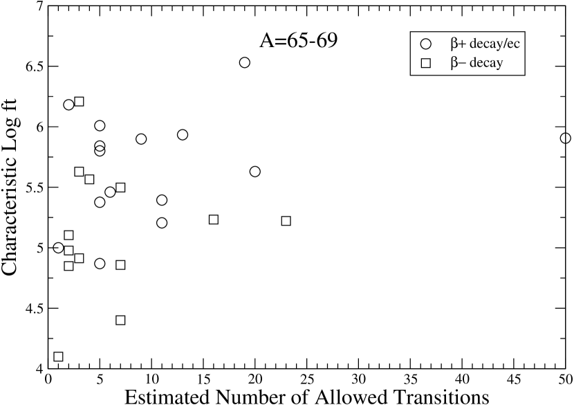
Figure 1: Systematics of experimentally-determined $\log ft$’s for nuclei with 65$\leq$A$<$70.

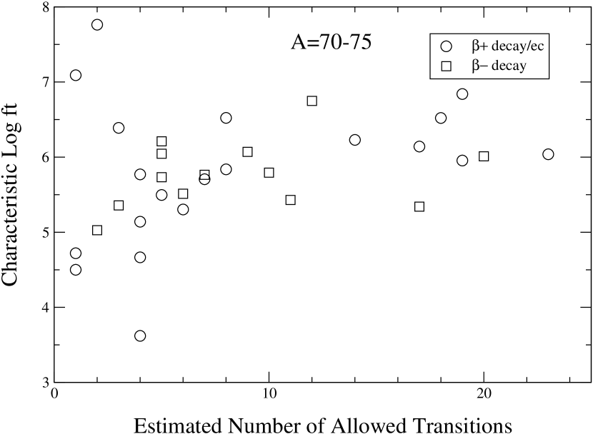
Figure 2: Systematics of experimentally-determined $\log ft$’s for nuclei with 70$\leq$A$\leq$75.

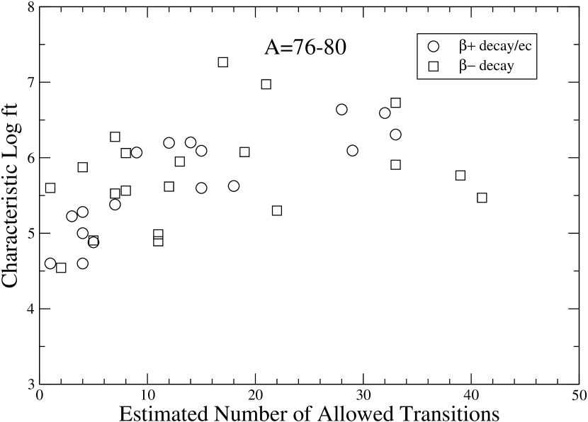
Figure 3: Systematics of experimentally-determined $\log ft$’s for nuclei with 75$<$A$\leq$80.

Figures 1, 2, and 3 show the characteristic $\log ft$ value for all nuclei in the mass range A=65-80 for which there is experimentally-determined weak decay information. By ”characteristic $\log ft$” we mean here the $\log ft$ value obtained by assuming that all of the measured discrete strength is spread uniformly over all states in the daughter for which the selection rules do not forbid a transition and for which the Q-value is positive. This estimated number of allowed transitions ($n_{\rm allow}$) for each nucleus is shown on the x axis. The determination of $n_{\rm allow}$ is difficult because of uncertainties in the angular momentum and spin assignments of levels. Where the angular momentum of a given level is uncertain we have adopted the middle value if more than two possibilities are listed, and the largest value if only two possibilities are given. Where the parity is listed, but uncertain, we have adopted the tentative value. Transitions involving a level for which no spin or parity information is given are labelled as forbidden.

For illustration, consider the $\beta$ decay of ${}^{66}{\rm Co}$. Experimentally it is observed that ${}^{66}{\rm Co}$ decays in this channel to two states in ${}^{66}{\rm Ni}$, one with a $\log ft$ of 4.21 and the other with $\log ft=$4.75. By examining the experimentally studied levels in ${}^{66}{\rm Ni}$ it is seen that there are 7 levels that have spins and parities consistent with allowed decay from ${}^{66}{\rm Co}$. The characteristic $\log ft$ for ${}^{66}{\rm Co}$ is then defined as $-\log_{10}((1/7)(10^{-4.21}+10^{-4.7}))$. Our definition of the characteristic $\log ft$ is rough in that it neglects the experimental difficulties associated with measuring weak transitions. In particular, uncertainties arising from the possibility of the feeding of daughter states from higher lying states has not been accounted for, nor has the difficulty of observing near-threshold transitions. Nonethless, a case may be made from these figures that the assumption of an average matrix element is a reasonable one, particularly when several transitions are involved. For example, for nuclei with $65\leq{\rm A}<70$, only one nucleus with $n_{\rm allow}>2$ has a characteristic $\log ft$ differing from 5.4 by more than 1, and for nuclei in the range $70\leq{\rm A}\leq 80$ only 5 nuclei with $n_{\rm allow}>2$ have a characteristic $\log ft$ differing from 5.7 by more than 1.

In this work we take a characteristic $\log ft$ of 5.4 for nuclei with A$<$70, and a characteristic $\log ft$ of 5.7 for nuclei with A$\geq$70. An alternative approach for estimating these matrix elements would be to assign $\log ft$’s from a statistical distribution. Our procedure should give a reasonable estimate of the rates when several transitions contribute nearly equally to the rate. However, our estimated rate is obviously subject to uncertainty when only one or two experimentally unknown transitions dominate. An important class of such nuclei are the proton-rich even-even nuclei with nearly closed neutron and proton sub-shells. These can have anomolously large $0^{+}\rightarrow 1^{+}$ GT transitions. In x-ray burst environments, with temperatures $T\sim 0.25{\,\rm MeV}$, the first $2^{+}$ excited state in these nuclei is thermally populated. The thermal $\beta^{+}$ decay rate of the nucleus depends sensitively on whether this $2^{+}$ state also decays with anomolously large matrix elements. Schatz et al. (1998) studied this question for a number of proton-rich nuclei and found that the $2^{+}$ state decays more rapidly than the ground state when the ground state decays quickly. We incorporate the results of the Schatz et al. (1998) shell model study for the four nuclei (${}^{72,74}{\rm Kr},^{76,78}{\rm Sr}$) with fast $0^{+}\rightarrow 1^{+}$ transitions. For these nuclei we assume that the first $2^{+}$ state has a strength distribution identical in shape, but with matrix elements twice as large, as the strength distribution from the $0^{+}$ ground state. This gives decay rates within $\sim 30\%$ of those calculated by Scahtz et al..

4 The Fermi and Gamow-Teller Resonances

The Fermi resonance $|F_{i}\rangle$ corresponding to a given state $|\psi_{i}\rangle$ is generated by application of the isospin raising or lowering operator, $|F_{i}\rangle=T_{\pm}|\psi_{i}\rangle$ (Eq. 10). The selection rules for Fermi transitions are $\Delta\pi=\Delta T=\Delta J=0$. Because $\Delta T=0$ and because the ground state of a nucleus generally has the lowest possible isospin, there typically is only non-zero Fermi strength for transitions from a nucleus with greater isospin $T^{>}$ to a nucleus with lesser or equal isospin $T^{<}$. Since the nuclear part of the Hamiltonian ($H_{\rm nuc}$) is isospin independent and the electromagnetic part is small in comparison, the resonance generated by $T_{\pm}$ is narrowly concentrated about the IAS. The excitation energy can be estimated from the difference in Coulomb binding energy of the parent and daughter nucleus. FFNI gives a useful approximation for the excitation energy of the IAS in the daughter nucleus:

$$E_{\rm IAS}=\Delta_{p}-\Delta_{d}\mp 0.7824\pm 1.728\min(Z_{p},Z_{d})/R$$ (15)

where $R\approx 1.12A^{1/3}+0.78$ is the nuclear radius in fm, p and d refer to the parent and daughter, respectively, $\Delta$ is the atomic mass excess. The upper signs in the above equation correspond to ${\rm(Z,N)\rightarrow(Z+1,N-1)}$ transitions for neutron rich parents, while the lower signs correspond to ${\rm(Z,N)\rightarrow(Z-1,N+1)}$ transitions for proton rich parents. Eq. 15 agrees well with measured and shell model predictions for IAS energies.

The Gamow-Teller operator is

$$GT_{\pm}=\sum_{n}{\bf\sigma}\tau^{\pm}(n),$$ (16)

where the sum is over all nucleons $n$. The collective GT resonance state $|{\rm CGT_{i}}\rangle$ corresponding to a given parent state $|\psi_{i}\rangle$ is given by application of the GT operator, $|{\rm CGT_{i}}\rangle=GT|\psi_{i}\rangle$. The selection rules for GT transitions are $\Delta\pi=0$, $\Delta J=0,\pm 1$ no $0\rightarrow 0$, and $\Delta T=0,\pm 1$. The GT strength distribution is harder to characterize because $H_{\rm nuc}$ is strongly spin dependent. Since $[H_{\rm nuc},GT_{\pm}]\neq 0$, the GT strength can be fragmented over many daughter states. However, in practice the stellar weak rates are usually determined by the total strength and the centroid of the strength in excitation energy (provided that low lying discrete transitions are well accounted for).

The strength in the GT resonance was also estimated by FFN in a zeroth order shell model picture. In this picture the lowest shell orbitals are filled with nucleons, and the total strength is taken to be the sum of the contributions from each pair of single particle orbitals:

$$|M_{\rm GT}|^{2}=\sum_{\rm if}{{n_{p}^{i}}{n_{h}^{f}}\over 2j_{f}+1}|M^{sp}_{\rm GT}|^{2}_{\rm if}.$$ (17)

Here i and f denote initial and final orbitals respectively, $n_{p}$ and $n_{h}$ denote the number of particles and holes in these orbitals, and $M^{sp}_{\rm GT}$ is the single particle matrix element connecting the initial and final states. These single particle matrix elements can be found from angular momentum considerations and are shown in Table 1 of FFNII.

We follow FFN in using the single particle result (Eq. 17) to estimate the total strength. Experimentally it is well established that the axial vector current is renormalized by a factor of $\sim(1/1.24)$ in nuclei. This results in a strength a factor of $(1/1.24)^{2}\approx 1/2$ smaller than shell model calculations give. In addition, shell model calculations show that residual interaction-induced particle-hole correlations further reduce the total strength by a factor of one to a few. Typically, these correlations are more important for ${\rm GT^{+}}$ transitions, so that the additional quenching is larger for these transitions. We adopt a quenching factor of 4 for ${\rm GT^{+}}$ transitions and 3 for ${\rm GT^{-}}$ transitions. These values for the quenching factors generally give strengths within a factor of two of more detailed strength determinations. When the quenched value for the strength is less than one, we assign a configuration mixing strength of one. As discussed below, this is roughly consistent with the results of (n,p) experiments for ${\rm GT^{+}}$ blocked nuclei.

FFN estimated the centroid of the GT resonance by considering a zeroth order shell model description for the spin flip part of the GT resonance. This configuration was compared with the zeroth order shell model description of the daughter ground state and assigned an excitation energy

$$E_{\rm GT}=\Delta E_{\rm s.p.}+\Delta E_{\rm pair}+\Delta E_{\rm ph}.$$ (18)

Here $\Delta E_{\rm s.p.}$ is the difference in single particle energies between the two states (daughter ground state and spin flip GT resonance state), $\Delta E_{\rm pair}$ accounts for the difference in pairing energy between the two states, and $\Delta E_{\rm ph}$ (taken to be 2 MeV) accounts for the effects of configuration mixing and particle hole repulsion. For $T^{>}\rightarrow T^{<}$ transitions the energy of the IAS in the daughter is added to eq. 18.

For the assignment of the GT centroids we adopt a procedure close to that outlined by FFN. However, as noted in the introduction, the FFN approach misses some important systematics in the centroids of the strengths as revealed by more recent experimental data and shell model calculations. One potential remedy for this is to do RPA or QRPA calculations for the strength distributions for nuclei too heavy to be studied via detailed shell model calculations. Such calculations have been done for a number of nuclei by several different groups. A simpler approach is to approximately account for the effects of the competition between the $k_{\sigma\tau}(\sigma_{1}\cdot\tau_{1})(\sigma_{2}\cdot\tau_{2})$ and $k_{\tau}(\tau_{1}\cdot\tau_{2})$ terms in the nuclear Hamiltonian. The effect of this competition on the centroid of the GT resonance is most easily seen in the Tamm Dancoff approximation from the argument given by Bertsch and Esbensen (1987). In this approximation the $k_{\tau}$ and $k_{\sigma\tau}$ forces give rise to a ${\rm GT^{-}}$ excitation energy scaling as

$$E_{\rm GT^{-}}\approx E_{\rm IAS}+\Delta E_{s.o}+2(k_{\sigma\tau}S_{GT^{-}}/3-(N-Z)k_{\tau}).$$ (19)

Here $\Delta E_{s.o.}$ is the spin orbit splitting characteristic of the single particle transitions for the ${\rm GT^{-}}$ resonance. As an example of this equation, consider the case of ${}^{54}{\rm Fe}$ and ${}^{56}{\rm Fe}$. The zeroth order $\beta^{-}$ strengths for these nuclei are $|M_{\rm GT}|^{2}=16.3$ ( ${}^{54}{\rm Fe}$) and 22.3 (${}^{56}{\rm Fe}$). For $k_{\sigma\tau}\sim(20/A){\rm MeV}\sim(2/3)k_{\tau}$, Eqn. 19 implies $(E_{GT^{-}}-E_{\rm IAS})_{{}^{56}{\rm Fe}}-(E_{GT^{-}}-E_{\rm IAS})_{{}^{54}{\rm Fe}}\approx-1\,{\rm MeV}$. Shell model calculations and (n,p) experiments for these nuclei give this difference as approximately -2 MeV. As Fe becomes more and more neutron rich $E_{\rm GT^{-}}$ approaches $E_{\rm IAS}$ and eventually falls below it (although perhaps beyond the neutron drip line for a nucleus as light as Fe).

A somewhat more sophisticated approach to incorporating the effects of the competition between the $k_{\tau}$ and $k_{\sigma\tau}$ forces is the random phase approximation with a separable force. In this approximation the GT⁺ and GT^- resonances become eigenstates of the Hamiltonian. The energies of the resonances are approximately given by the roots of the algebraic equation

$${f_{1}\over\epsilon_{i}-\epsilon+\Delta_{\rm s.o.}^{-}}+{f_{2}\over\epsilon_{i}-\epsilon}+{f_{3}\over-\epsilon_{i}+\epsilon+\Delta_{\rm s.o.}^{+}}=-{3\over 2}{1\over k_{\sigma\tau}}{1\over S_{\rm tot}}$$ (20)

(see Gaarde et al. (1981) for an application of this equation to experimentally observed $\beta^{-}$ strengths, or Rowe (1970) for a more pedagogical discussion). In Eq. 20, $S_{\rm total}=S_{\rm GT^{-}}+S_{\rm GT^{+}}=3|N-Z|+2S_{\rm GT^{+}}$ is the sum of the strengths in the plus and minus directions, $f_{1}$ is the fraction of this strength in the ${\rm GT^{-}}$ spin-flip mode, $f_{2}$ is the fraction of this strength in the ${\rm GT^{-}}$ non-spin flip mode, and $f_{3}$ is the fraction of strength in the ${\rm GT^{+}}$ direction. The spin orbit splittings $\Delta^{+}_{\rm s.o.}$ and $\Delta^{-}_{\rm s.o.}$ are the splittings appropriate for the spin flip transitions in the plus and minus directions, $\epsilon_{i}=(\epsilon_{\pi}-\epsilon_{\nu})_{i}$ is the difference in the proton and neutron single particle energies for the levels involved in the transition. The quantity $\epsilon_{i}$ is related to the energy of the IAS by $E_{\rm IAS}-\epsilon_{i}=2k_{\tau}|N-Z|$. The largest root of Eq. 20 corrresponds to the energy of the spin flip mode. Eq. 20 reduces to Eq. 19 in the limit $f_{1}=1$.

Our approach for calculating the centroid of the ${\rm GT^{-}}$ resonance is based on Eq. 20. The strengths in this equation are estimated in the zeroth order shell model picture described above. For consistency with FFN we take the spin orbit splittings from Seeger and Howard (see the table in Hillman and Grover (1969)). When more than one spin flip transition contributes to the strength we take the strength-weighted average. The parameter $k_{\tau}$ can be estimated using measured IAS energies and estimates for the particle-hole energies. Alternatively, an estimate for the IAS energy (Eq. 15) gives a relation between $k_{\tau}$ and $\epsilon_{i}$. The parameter $k_{\sigma\tau}$ can be chosen to give good agreement with shell model and experimental results for the ${\rm GT^{-}}$ resonance in the fp shell. In this work we adopt $k_{\tau}=28.5/{\rm A}{\,\,\rm MeV}$ and $k_{\sigma\tau}=23/{\rm A}{\,\,\rm MeV}$. These values are close to those given in Bertsch and Esbensen (1987) and Gaarde et al. (1981). It has previously been noted by a number of authors (e.g. Gaarde et al. (1981)) that a simple prescription can do a fair job of predicting the centroids of the ${\rm GT^{-}}$ resonances. In table 2 we reaffirm this by comparing the predictions based on Eq. 20 with measured and shell model results.

For the ${\rm GT^{+}}$ resonance, estimates based on a separable force are not well justified. Higher order particle hole correlations and correlations induced by other terms in the Hamiltonian play a more important role. Nonethless, the RPA result accounts for the spin orbit splittings and the systematics of the influence of the $k_{\tau}$ and $k_{\sigma\tau}$ forces in an approximate way. We estimate the centroid of the ${\rm GT^{+}}$ resonance from the equation analogous to Eq. 20 (which is found by reversing the role of the plus and minus transitions, and by setting $\epsilon_{i}=(\epsilon_{\nu}-\epsilon_{\pi})$ or alternatively by setting $\epsilon\rightarrow-\epsilon$ in Eq. 20). We also add an additional term to account for the effects of correlations missed by the separable force estimate:

$$E_{\rm GT^{+}}=E_{\rm GT^{+},RPA}+\delta_{\rm ph}.$$ (21)

A value of 2 MeV for the empirical correction $\delta_{\rm ph}$ gives good agreement with the results of experimental and shell model studies of nuclei in the lower half of the fp shell. This is demonstrated in Table 3.

Our simple estimate for $E_{\rm GT^{+}}$ probably breaks down as the fp shell approaches being filled. Fortunately, for most nuclei in this case ($A>65$) the ${\rm GT^{+}}$ transition is nearly blocked (see below). Likewise, for those proton rich nuclei with substantial amounts of unblocked strength the electron capture Q-value is large, so again the rate is not terribly sensitive to assumptions about the centroid. For the few proton-rich nuclei with modest ${\rm GT^{+}}$ strength, we can compare our results to the more detailed QRPA calculations of Sarriguren et al. (2001). These authors performed QRPA studies for even-even Ge, Se, Kr, and Sr isotopes. For the most part their calculated electron capture half lives agree well with experimental half lives.

For ⁶⁶Ge, ⁶⁸Ge, and ⁷⁰Se Sarriguren et al. (2001) find that the strength distribution is not very sensitive to which of two nearly degenerate shapes the nucleus assumes, so that a direct comparison with our estimate is sensible. For these nuclei our estimate for the centroid of the resonance is lower than theirs by 1.5 Mev(⁶⁶Ge), 1.8 MeV (⁶⁸Ge), and 2.5 MeV (⁷⁰Se). For some of these nuclei it is not clear which estimate is correct. Sarriguren et al. (2001) show that their method gives a centroid about 2 MeV higher than the experimental centroid for ⁵⁴Fe and ⁵⁶Fe, and that there calculation for ⁷⁰Ge misses a modest amount of experimentally-determined low lying strength.

However, in at least one case (⁷⁰Se), our assignment of the strength is at least 0.5-1 MeV too low, because it results in too much strength within the electron capture window and results in a half life about 5 times shorter than the experimentally determined half life. (Note though, that where a half life is available for a nucleus our calculations always agree with that half life. We do not include resonance strength below the Q-value window for a transition when experimental information is available.) We will argue in the last section that the uncertainty in the placement of the centroid of the ${\rm GT^{+}}$ strength is not very important for nuclei in the mass range we are considering.

As the ${\rm GT^{+}}$ strength decreases (i.e., as an isotope becomes more neutron rich), Eq. 21 eventually gives a negative excitation energy for the resonance in the daughter. This typically happens when the single particle estimate for the strength (Eq. 17) is less than about 5. In this case, the strength is dominated almost entirely by configuration mixing. There are a few (n,p) studies of such nearly blocked nuclei. Vetterli et al. (1992) studied ${}^{70}{\rm Ge(n,p)}^{70}{\rm As}$ and ${}^{72}{\rm Ge(n,p)}^{72}{\rm As}$. The experimentally-determined GT strength for ${}^{70}{\rm Ge}$ is B(GT)=$0.84\pm 0.13$ or B(GT)=$0.72\pm 0.14$. The two different values correspond to different ways of estimating the $\Delta{\rm L}=0$ component of the (n,p) cross section. The higher estimate comes from a multipole decomposition (m-d) of the cross section, while the smaller estimate is derived by approximating the cross section measured at $5.8^{\circ}$ as the $\Delta{\rm L}=1$ component of the cross section. For the m-d the strength distribution for ${}^{70}{\rm Ge}$ is approximately flat up to a few tens of MeV in excitation energy in ${}^{70}{\rm As}$. For the $5.8^{\circ}$ subtraction method, the strength falls after about 6 MeV in excitation energy in ${}^{70}{\rm As}$. For ${}^{72}{\rm Ge}$ B(GT)=$0.23\pm 0.05$ ($5.8^{\circ}$) or B(GT)=$0.86\pm 0.14$ (m-d) and the strength distribution is roughly flat or falls off after about 6 MeV depending on the background substraction method. Helmer et al. (1997) have studied ${}^{76}{\rm Se}{\rm(n,p)}^{76}{\rm As}$. They find B(GT)=1.45 with a roughly flat strength distribution for the m-d method, and B(GT)=0.35 with a strength extending to about 6 MeV in ${}^{76}{\rm As}$ if the $6^{\circ}$ data is used to estimate the $\Delta{\rm L}=1$ component of the cross section. In this work we adopt the procedure that when the RPA estimate $E_{\rm GT^{+},RPA}$ appearing in Eqn. 21 is negative with respect to the daughter ground state, the strength distribution is represented by a 1 MeV gaussian centered at 1.8 MeV. This is approximately consistent with the experimental data analyzed using the $5.8^{\circ}$ ($6^{\circ}$) background substraction method. Our prescription misses the high lying strength estimated from the experimental data analyzed using the multipole decomposition method. We will discuss in the last section the uncertainties in the rates resulting from the unknown strength distribution for these blocked nuclei.

5 Thermal considerations

The picture for Fermi and Gamow-Teller strengths outlined above becomes more complicated at high temperatures on account of the thermal population of parent excited states. In evaluating the contribution to the rates of transitions between low lying levels, we use the same set of experimentally-determined levels discussed above.

As the temperature rises, the evaluation of Eq. 1 requires knowing the strength distributions of an impossibly large number of states. For example, at temperature of $1\,{\rm MeV}$ the partition function for an odd-odd nucleus with $A\approx 60$ is a few hundred, and the mean excitation energy is $T^{2}\rho_{\rm F}\approx T^{2}A/8\approx 7\,{\rm MeV}$ (here $\rho_{\rm F}\approx a$ is the level density at the fermi surface and $a\approx A/8$ is the level density parameter). The approximation traditionally (see FFNII) used to make the problem tractable is the Brink approximation, which postulates that the centroid of the Gamow-Teller strength distribution corresponding to a parent state at excitation energy $E_{i}$ is shifted up by an energy $E_{i}$ with respect to the centroid of the strength distribution corresponding to the parent ground state. It is generally assumed that the total strength remains the same for all transitions. The validity of the Brink approximation has been investigated in some detail by LMP. They find that the approximation is good for the first few low lying states for which they calculate strength distributions.

With the Brink approximation, the contribution of discrete state to high lying resonance state transitions can be approximated. For definiteness we assume in the following discussion that the parent nucleus has isospin $T^{>}$, the daughter nucleus has isospin $T^{<}$, and that the GT^- operator acting on the parent generates states in the daughter (and conversely). Each parent state ($|\psi_{i}^{\rm P}\rangle$) has a corresponding Fermi resonance ($|F_{i}\rangle=T^{-}|\psi_{i}^{\rm P}\rangle$) and collective Gamow-Teller resonance ($|CGT_{i}\rangle=GT^{-}|\psi_{i}^{\rm P}\rangle$) in the $T^{<}$ daughter. With the Brink approximation, the Q-values for these transitions are independent of the excitation energy of the thermally populated parent state. The overall transition rate for these processes can be obtained brom a calculation of the ground state rate alone, but with the population factor of the ground state set to unity. This is part of the “FFN trick”.

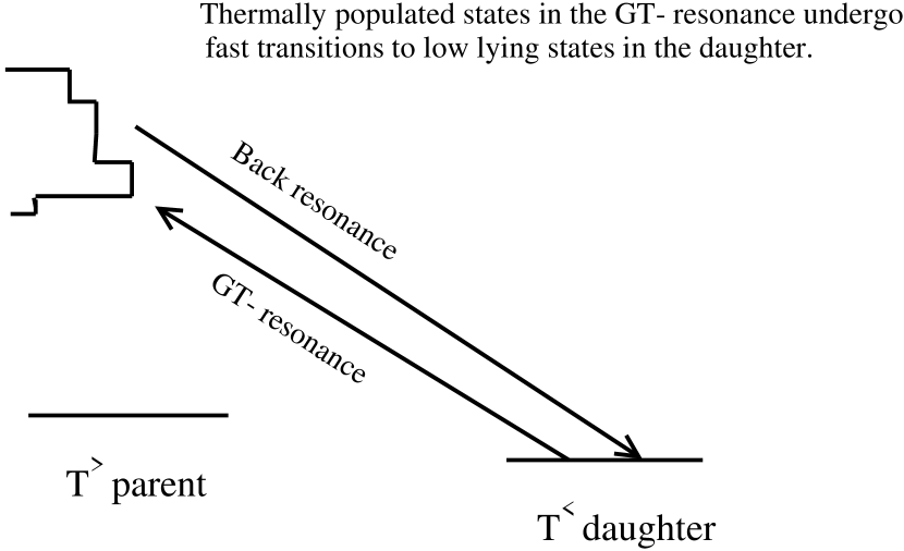
Figure 4: Illustration of the position and energetics of discrete state-resonance transitions (back resonances).

Likewise, it is possible to thermally populate the collective Gamow-Teller states in the $T^{>}$ parent ($|CGT_{j}\rangle=GT^{+}|\psi_{j}^{\rm D}\rangle$). These thermally populated states can decay to the daughter with large overlap. These “back-resonances” are shown in Fig. 4. Suppose for a moment that the GT⁺ resonance corresponding to a state in the daughter is confined to a single state in the parent. In this case the Brink approximation implies that for each state with excitation energy $E_{\rm daughter,j}$ in the daughter, there is a corresponding GT⁺ resonance state ($|CGT_{j}\rangle=GT^{+}|\psi_{j}^{\rm D}\rangle$) in the parent with excitation energy $E_{0}+E_{\rm daughter,j}$. Here $E_{0}$ is the excitation energy in the parent of the resonance state corresponding to the daughter ground state. Because in the Brink approximation the Q-values and strengths for all the transitions $(E_{0}+E_{j})_{\rm parent}\rightarrow(E_{j})_{\rm daughter}$ are the same, the rate contribution for each transition is also the same and can be written as $\bar{\lambda}$. The contribution of the back resonances to the rates can be directly evaluated:

$$\lambda_{\rm backres}={\bar{\lambda}\sum_{i}\exp(-E_{\rm parent,i}/T)(2J_{\rm parent,i}+1)\over Z_{\rm parent}}\\$$ (22)

$$\approx{\bar{\lambda}\sum_{j}\exp((-E_{\rm daughter,j}+E_{0})/T)(2J_{\rm daughter,j}+1)\over Z_{\rm parent}}\\$$

$$=\bar{\lambda}\exp(-E_{0}/T){Z_{\rm daughter}\over Z_{\rm parent}}.$$

Eq. 22 was first derived in FFNII and is sometimes referred to as the “FFN trick”.

In this work we represent the resonance strength distribution by a gaussian of nominal width $\sigma$. For the ${\rm GT^{+}}$ strength distribution we take $\sigma=1\,{\rm MeV}$ and for the ${\rm GT^{-}}$ strength distribution we take $\sigma=2\,{\rm MeV}$. This approximation does not fairly represent the complex structure and variation seen in real strength distributions. However, we will see in the last section that this simple approximation captures the features relevant for calculations of weak rates in a stellar environment. The case where the resonance is spread over several states in the parent can be treated similarily to the case where the resonance is concentrated in a single state. If the resonance corresponding to the ground state in the daughter is spread over states with excitation energy $E_{0},E_{1},...E_{n}$ in the parent, with corresponding rates to the daughter ground state given by $\bar{\lambda}_{0j}$, then Eq. 22 becomes

$$\lambda_{\rm backrate}\approx{\sum_{j}\bar{\lambda}_{0j}\exp(-E_{0j}/T)Z_{\rm daughter}\over Z_{\rm parent}}.$$ (23)

This equation is exact in the limit where the Brink approximation holds (i.e., the strength distribution from every daughter state is identical to the strength distribution from the daughter ground state except for an overall shift in energy). The interesting feature of Eq. 23 is that if all of the Q-values for the n states are comparable, then

$$\lambda_{\rm backrate}\approx n\langle\bar{\lambda}_{0j}\rangle\exp(-E_{0}/T)Z_{\rm daughter}/Z_{\rm parent}=\bar{\lambda}\exp(-E_{0}/T)Z_{\rm daughter}/Z_{\rm parent},$$ (24)

independent of n. Here the relation $n\langle\bar{\lambda}_{0j}\rangle\approx\bar{\lambda}$ (where $\bar{\lambda}$ is the rate of decay calculated assuming that the GT resonances are confined to single states) holds because the total strength in the GT resonance is independent of the number of states it is spread over. In a sense Eq. 24 is counterintuitive because one might expect that if the strength is spread out over n states in the parent, the decay rate from the parent should be a factor of 1/n smaller. However, in some cases the strength distributions arising from different states in the daughter must overlap (i.e. correspond to identical states in the parent) to the extent that the level densities in the parent and in the daughter are comparable. This is accounted for by the ratio of partition functions appearing in Eq. 23.

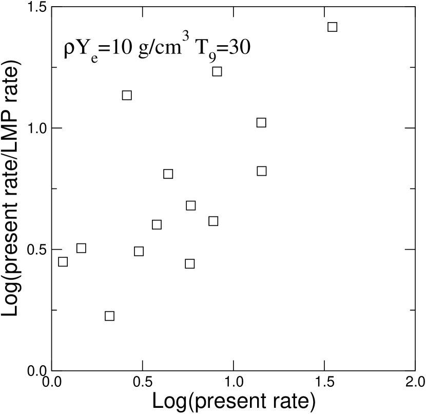
Figure 5: Comparison of our $\beta^{-}$ decay rates with the LMP rates for nuclei in the mass range A=60-65. The comparison is made at $T_{9}=30$, $\rho Y_{e}=10{\rm g/cm^{3}}$. These conditions are artificial but serve to illustrate the influence of the treatment of the partition function on estimates of the weak rates. In all plots where a rate is shown the rate is in units of ${\rm sec^{-1}}$.

In principal, the back resonance contribution to the rates could be calculated through a direct (e.g., shell model) calculation of the strength distribution from the daughter states. In practice this approach is not feasible because such a calculation would have to have fully converged final states corresponding to the strength distribution from many daughter states in order to distinguish which ones are identical. Otherwise, an overcounting of the partition function results, and the final rate estimate is a function of how many Lanczos iterations are done. This line of reasoning indicates that at high temperatures the current shell model-based calculations could systematically underestimate the contribution to the $\beta$ decay rates from the decay of the thermally populated ${\rm GT^{+}}$ resonance states by up to an order of magnitude. To show this, we plot in Fig. 5 a comparison between our calculated $\beta^{-}$ decay rates and those of LMP at a temperature of $T_{9}=30$ and a density of $\rho Y_{e}=10{\rm g/cm^{3}}$. These thermodynamic conditions are artificial, but serve the purpose of illustration. When the $\beta$ decay rate is fast (and insensitive to the finer details of the strength distribution), the discrepancy between the two calculations is about a factor of 10. This is roughly the number of independent Lanczos states carrying strength per daughter state in the calculations of LMP. From our simple analysis it isn’t clear that either set of rates is more reliable. However, it is clear that differences in treatments of the partition functions can result in significant differences in estimates of the rates.

The trend of greater disagreement with faster decay rate seen in Fig. 5 arises from the competition of two factors. For low decay rates, the Q-value of the decay (excitation energy of the ${\rm GT^{+}}$ resonance with respect to the daughter ground state), is typically small. In this case the width of the resonance enhances the decay rate compared to the decay rate calculated from our artificially narrow resonance. For faster decay rates, the Q-value is large, the lifetime is relatively insensitive to the width of the resonance, and the Lanczos-based calculation rate estimate is simply suppressed by the overestimate of the parent partition function.

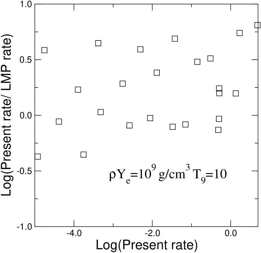
Figure 6: Same as Fig. 5 but at $T_{9}=10$, $\rho Y_{e}=10^{9}{\rm g/cm^{3}}$, conditions approximating the post Si burning degenerate core before collapse.

The effect, and the importance of consistency in partition functions in general, can be illustrated by considering the conditions in the post-silicon burning, pre-collapse core of a massive star. There electron capture proceeds on iron peak nuclei, driving them to a neutron excess where “reverse” $\beta^{-}$ decay balances “forward” electron capture. For example, Aufderheide et al. (1994) identify ${}^{64}{\rm Cr}$ as the endpoint nucleus where the forward and reverse neutronization rates balance. In balanced conditions, partition functions are crucial rate and abundance determinants. We can compare our rates with LMP as in Fig. 5, but now for $T_{9}=10$, $\rho Y_{e}=10^{9}{\rm g/cm^{3}}$, roughly approximating immediately pre-collapse conditions. This comparison is shown in Fig. 6. Again there is a systematic trend: the LMP rates are lower than ours by a factor of 4 on average with a fair scatter. This is smaller than the disagreement presented above for the fastest $\beta$ decay rates, but still of potential significance given the dependence of the initial ${\rm Fe}$ core mass on the electron fraction. Part of the discrepancy between the rate estimates undoubtedly stems from differences in placement and width of GT strength and other nuclear uncertainties.

However, the partition effect outlined above likely plays a role as well. In fact, these conitions ($T_{9}=10$, $\rho Y_{e}=10^{9}{\rm g/cm^{3}}$) are electron degenerate with Fermi energies $\sim 5{\,\,\rm MeV}$, precluding significant $\beta$ decay for all but the nuclear decay pairs with relatively large Q-values, just those where we argued that the partition function-based uncertainties in rate estimates could be large.

In evaluating the ratio $Z_{\rm daughter}/Z_{\rm parent}$ in Eq. 23 we use the compilation of partition functions from Rauscher and Thielemann (1999). These partition functions include experimentally-determined low lying levels and are supplemented at higher excitation energies by a level density calculated from a back shifted Fermi gas formula. At low temperatures the partition functions of Rauscher and Thielemann (1999) agree well with the partition functions we calculate for evaluating the rates between low lying levels. For temperatures above 2 MeV we take $Z_{\rm daughter}/Z_{\rm parent}=1$. This is valid because the mean excitation energy at these temperatures is well above the pairing gap.

We do not claim that our partition function treatment is necessarily better than others, and it may well be inadequate in some conditions. In fact there is a basic inconsistency in our rates: we include many states in our partition function sums for which we include no weak interaction strength. Ideally we should include all states and all associated weak strength: only fully converged Lanczos and Monte Carlo calculations of weak strength and partition functions currently do this. Failing to estimate partition functions and strength functions consistently can lead to inaccurate predictions of final ${\it equilibrium}$ parameters. In equilibrium, the hard won rates no longer matter and only the partition functions govern the final quantities of interest ($Y_{e}$, abundances, etc.).

6 Results and Discussion

6.1 A validity test: Comparison with Shell Model Based Rates for A=60-65

Here we address the reliability of our calculated rates. We have shown in section 3 that with a simple prescription some gross features of the strength distribution, in particular the total strength and centroid of the distribution, may be estimated. However, shell model and experimental results typically show a rich structure in the strength distribution, with this structure varying markedly from nucleus to nucleus (e.g. Caurier et al. (1999)). Do the rates depend sensitively on the finer features of the strength distribution? Or, alternatively, can a computationally simple method give a good estimate of the weak interaction rates? These questions can be addressed by comparing our relatively simply derived rates with rates based on more detailed large dimension shell model calculations.

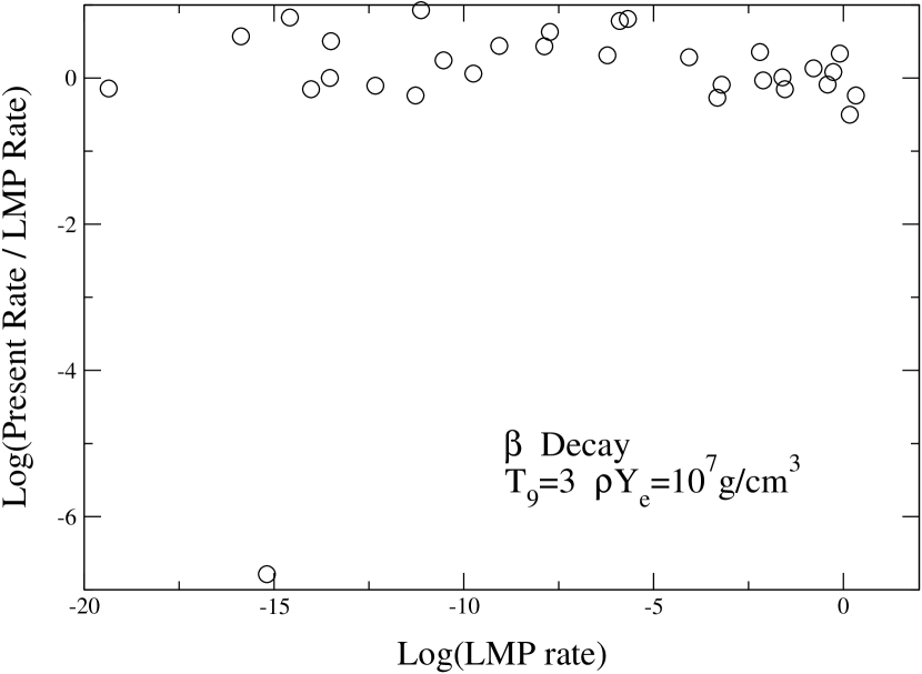
Figure 7: Comparison of our beta decay rates calculated using a simple estimate of the strength distribution with the more sophisticated calculations of Caurier et al. (1999) and Langanke and Martinez-Pinedo (2000). The different circles correspond to different nuclei. Comparisons for all nuclei in the mass range A=$60-65$ for which Langanke and Martinez-Pinedo (2000) provide rates are presented. Here $T_{9}=3$ and $\rho Y_{e}=10^{7}{\rm g/cm^{3}}$.

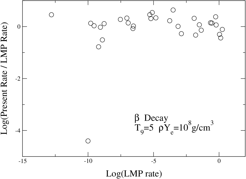
Figure 8: Same as figure 7 but with $T_{9}=5$ and $\rho Y_{e}=10^{8}{\rm g/cm^{3}}$

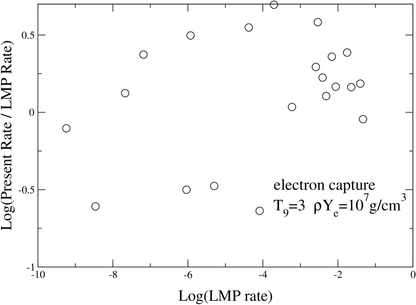
Figure 9: Comparison of our electron capture rates with those of Langanke and Martinez-Pinedo at $T_{9}=3$, $\rho Y_{e}=10^{7}{\rm g/cm^{3}}$. Only results for nuclei that are estimated by LMP to have electron capture rates larger than $10^{-10}{\rm sec^{-1}}$ are shown.

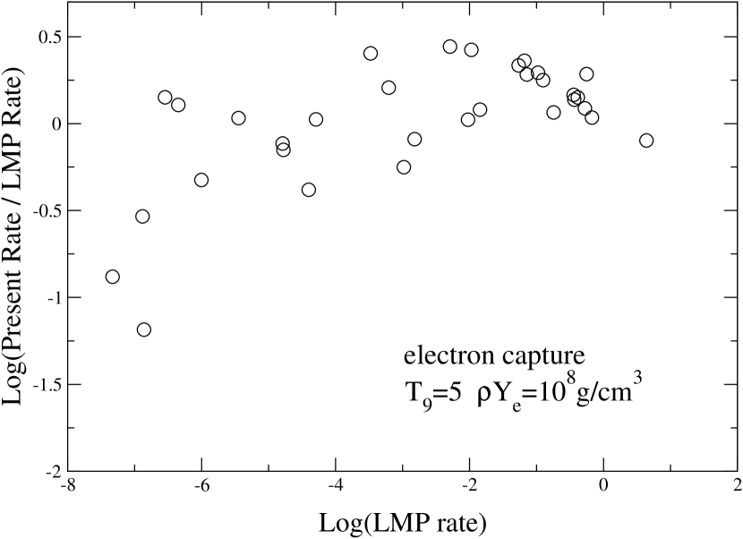
Figure 10: Same as figure 9 at $T_{9}=5$ and $\rho Y_{e}=10^{8}{\rm g/cm^{3}}$.

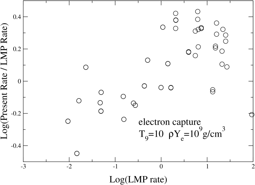
Figure 11: Same as figure 9 at $T_{9}=10$ and $\rho Y_{e}=10^{9}{\rm g/cm^{3}}$.

In figures 7 and 8 we show the log of the ratio of our calculated beta decay rates to those calculated in Langanke and Martinez-Pinedo (2000) at several temperature/density points relevant for stellar collapse, and for all nuclei in the range A=60-65 for which LMP calculated rates. The horizontal axis in this figure is the log of the beta decay rate calculated by LMP. We have presented the comparison in this way because nuclei with very small rates will not be so important in determining the evolution. The comparison is generally remarkably favorable, with typical results differing by less than a factor of two. Figures 9,10 and 11 are the same as the previous three figures, but now electron capture rates are being compared. Again, the comparison is favorable, the rates as calculated in the two schemes being within a factor of three or so. This is surprising given the potential sensitivity of electron capture rates to the placement and the width of the Gamow-Teller distribution.

The fact that a simple prescription and rough estimates of the strength do a reasonably good job in getting the rates relevant for stellar collapse is not to say that all rates are accurately determined at all temperatures and densities with a simple model. Some of our calculated rates deviate significantly from more detailed calculations. This typically occurs for $\beta^{-}(\beta^{+})$ decay when thermal population of the states in a collective Gamow-Teller resonance results in an exponential sensitivity, or for lepton capture when the maximum lepton energies are just on the edge of being able to reach the resonance in the daughter. Typically this exponential sensitivity is accompanied by a very small rate, so that it is not very important for stellar evolution.

6.2 Examples of some rates important in X-ray burst environments

X-ray bursts arise from the thermonuclear burning of hydrogen and helium accreted onto the surface of a neutron star in a binary system (see Wallace and Woosley (1981)). Characteristic temperatures during burning are a few hundred keV, and characteristic densities are $\rho Y_{e}\approx 10^{6}{\rm g/cm^{3}}$. The creation of nuclei heavier than ${\rm A}\approx 40$ occurs via the rp-process, in which nuclei undergo $({\rm p,\gamma})$ reactions until they approach the proton drip line and/or $\beta^{+}/{\rm ec}$ decay intervenes. The time for burning along the rp-process path is set to some extent by the $\beta^{+}/$ec lifetime of a few important waiting point nuclei. Here we present a few examples of important rates.

Three important waiting point nuclei with A$<$80 are the even-even (proton bound) nuclei ${}^{64}{\rm Ge}$, ${}^{68}{\rm Se}$, and ${}^{72}{\rm Kr}$ (Schatz et al., 2001). For each of these nuclei the single proton capture daughter (Z+1,N) is unbound, while the next heaviest isotone (Z+2,N) is bound. At low temperatures $(T_{9}\lesssim 1.5)$ the weak rate most important for determining flow towards the valley of $\beta$ stability is $\lambda_{\beta^{+}}$(Z,N). For higher temperatures an equilibrium between (Z,N) and (Z+2,N) is reached, so that $\lambda_{\beta^{+}}(Z+2,N)$ is also important. As a typical example we discuss ${}^{72}_{36}{\rm Kr}$ and it’s two-proton capture daughter ${}^{74}_{38}{\rm Sr}$.

The first $2^{+}$ excited state of ${}^{72}{\rm Kr}$ lies at $\approx 700\,{\rm keV}$ and is not significantly populated for temperatures $T_{9}<2.5$. The ground state lifetime of ${}^{72}{\rm Kr}$ is experimentally-determined. The low lying strength distribution in the daughter (${}^{72}{\rm Br}$) has also been measured. With the ground state lifetime and low lying strength distribution measured, the only missing piece of information is the strength distribution at excitation energies too high to be experimentally observed. Our rough estimate (Eq. 21) places a sizable portion of the resonance strength within the Q-value window for the decay. In order not to conflict with the experimentally-determined lifetime we push this strength up to Q=0 in our calculation.

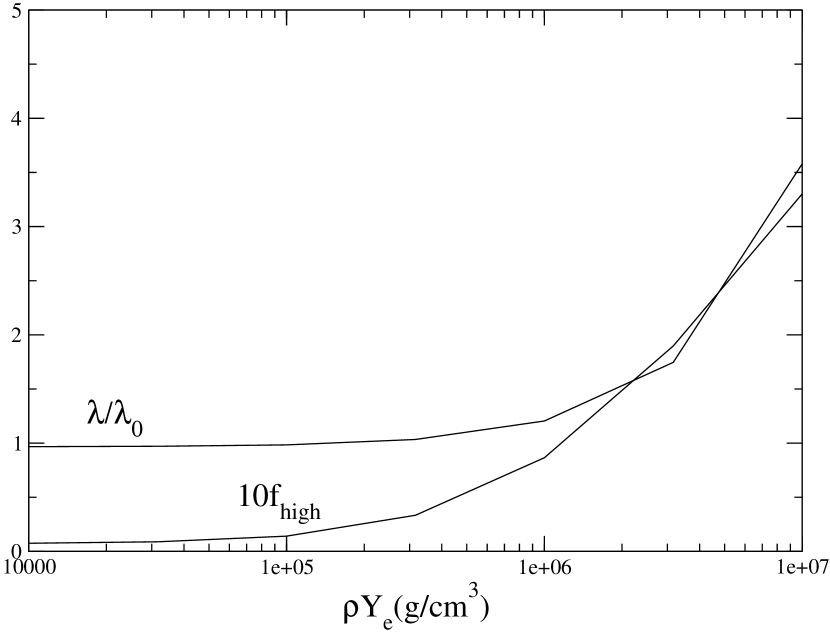
Figure 12: Influence of high lying resonance strength on the total rate ($\beta^{+}+ec$) for ${}^{72}{\rm Kr}$. In this figure $f_{\rm high}$ is an estimate of the fraction of the total rate arising from transitions involving experimentally unmeasured, high lying resonance strength. The upper curve, labelled $\lambda/\lambda_{0}$, shows the ratio of the total rate to the $\beta^{+}$ decay rate at zero temperature.

To quantify the uncertainty in the rates arising from the high lying resonance strength we plot in Fig. 12 the total rate (${\beta^{+}+{\rm ec}}$) for ${}^{72}{\rm Kr}$. Also included in this figure is the fraction of the total rate coming from Q=0 and above. The figure shows that the experimentally-determined lifetime is sufficient for a determination of the thermal decay rate at the $10\%$ level for $\rho Y_{e}<10^{7}{\rm g/cm^{3}}$. At $\rho Y_{e}=10^{7}{\rm g/cm^{3}}$, our simple estimate shows the high lying strength accounting for $\sim 20\%$ of the total weak rate. Because our method puts essentially all of the strength at Q=0, and very little above Q=0, it is unlikely that we have underestimated the contribution to the rate from the high lying resonance strength.

The decay of ${}^{74}{\rm Sr}$ is more easily calculated because the ground state (or a low lying excited state) of the odd-odd N=Z daughter (${}^{74}{\rm Rb}$) is the IAS of the ground state of ${}^{74}{\rm Sr}$. The large matrix element and Q-value ($\sim 10\,{\rm MeV}$) for the Fermi decay mean that electron capture cannot compete with $\beta^{+}$ decay in x-ray burst conditions for this case. It is difficult to reliably estimate the contribution to the $\beta^{+}$ rate from ${\rm GT^{+}}$ transitions, but a reasonable estimate is that the diffuse ${\rm GT^{+}}$ strength only decreases the ground state lifetime by at most $10-20\%$.

By mirror symmetry, a low lying thermally populated state of ${}^{74}{\rm Rb}$ corresponds to the IAS of the next even-even $\beta^{+}$ nucleus (${}^{74}{\rm Kr}$), so that the chain ${}^{74}{\rm Sr}\rightarrow^{74}{\rm Rb}\rightarrow^{74}{\rm Kr}$ is fast and dominated by Fermi transitions. The decay of the odd-odd N=Z nucleus (${}^{74}{\rm Rb}$ in this example) should is calculated as the decay of a thermally populated back resonance as discussed above. This is because only those parent states with an IAS in the even-even daughter nucleus decay via the Fermi transition. Since the partition function of the odd-odd parent increases more rapidly with temperature than the partition function of the even-even daughter, the decay rate decreases rapidly with increasing temperature. Another set of nuclei important for the rp-process with decays dominated by the Fermi transitions are those nuclei with ${\rm(Z=N+1,N=even)}$. These have an IAS near or at the ground state of the $\beta^{+}$ daughter.

Generally, for a given ground state lifetime, the electron capture rate is small and insensitive to the placement of strength within the Q-value window as long as the initial state electron energy is small compared to the energy of the decay, i.e.

$$\langle E_{e}\rangle<({\rm M_{p}-M_{d}+E_{i}-E_{f}}).$$ (25)

In the x-ray burst environment $\langle E_{e}\rangle<0.5\,{\rm MeV}$, while the Q-values for the proton-rich nuclei are typically greater than $4\,{\rm MeV}$, so the thermal lifetime is reliably estimated from the ground state lifetime. By contrast, nuclei closer to the valley of stability have smaller Q-values and therefore the lifetimes are nearly entirely determined by thermal electron capture.

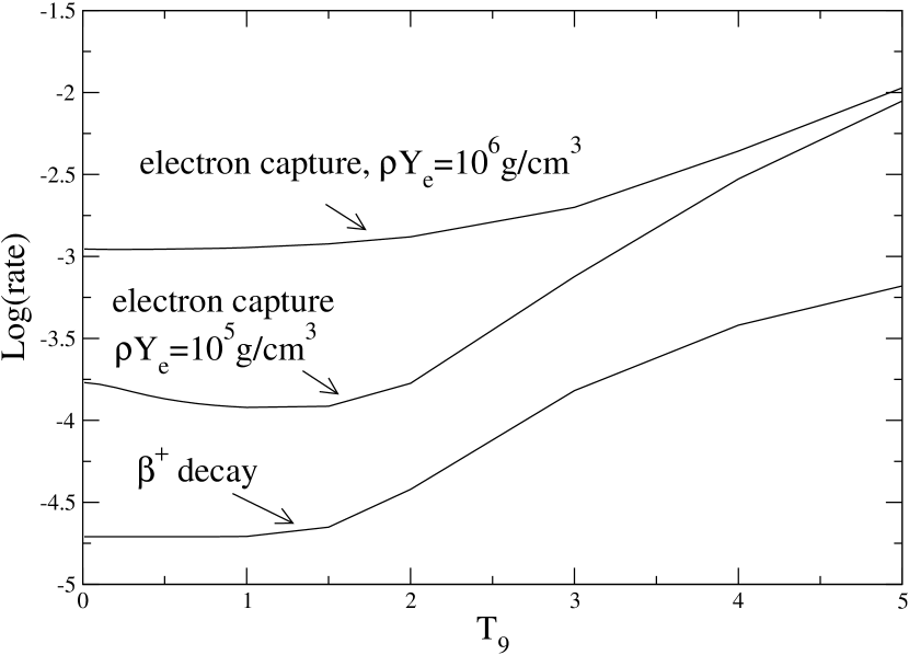
Figure 13: $\beta^{+}/{\rm ec}$ rates for ${}^{66}{\rm Ge}$.The increase of the $\beta^{+}$ rate with temperature arises from the fast decay of the thermally populated first $J^{\pi}=2^{+}$ excited state. Unlike the $0^{+}$ ground state, the $2^{+}$ state can have allowed transitions to several $2^{+}$ and $3^{+}$ daughter states. The decrease in the electron capture rate at low temperatures is likely an artifact of our calculation and arises because the $0^{+}$ ground state has substantial ${\rm GT}$ strength at high daughter excitation energies. As the daughter level structure is poorly known at these high excitation energies, our calculation does not include estimates of the allowed matrix elements for the decay of the first excited $2^{+}$ state to those states.

For example, consider ${}^{66}{\rm Ge}$, a nucleus important in steady state burning on and/or near neutron star surfaces. This nucleus has a Q-value of only $\sim$2 MeV and a fair portion of the strength lies at the upper end of the Q-value window. Consequently thermal electron capture dominates over positron decay for $\rho Y_{e}\gtrsim 10^{5}{\rm g/cm^{3}}$. This is shown in figure 13.

6.3 Weak rates in the late time pre-supernova star

Here we discuss some of the systematics of the weak rates in the hot and electron-degenerate core during the $\sim 10^{4}$s before core bounce. Most of the nuclei with A$>$65 present in the core will be blocked or nearly blocked to $GT^{+}$ transitions in the zeroth order shell model picture. Our calculation of the electron capture rates for these nuclei is based on an estimate of the $GT^{+}$ configuration mixing strength. Forbidden transitions and transitions allowed by the thermal unblocking of strength will also contribute to the electron capture rates. It is useful to estimate how large the configuration mixing strength must be in order to justify the neglect of these latter types of transitions.

Thermal unblocking refers to the population of parent excited states that have zeroth order shell model configurations consistent with allowed transitions to states in the daughter. Assume that these parent states comprise a fraction $\delta Z$ of the total partition function. Then, an effective thermal unblocking matrix element is $|M_{\rm TU}|^{2}\approx(\delta Z/Z)|M_{\rm s.p.}|^{2}$. Here $|M_{\rm s.p.}|^{2}\approx 1-3$ is a typical single particle allowed transition matrix element. An accurate estimate of $\delta Z$ is very difficult and an important open issue. Fuller 1982 parametrizes $\delta Z\approx Zexp(-E^{*}/T)$, with $E^{*}$ the excitation energy of the lowest parent excited state with an allowed $GT^{+}$ transition in the zeroth order shell model picture. With this schematic notation, thermal unblocking can compete with a configuration mixing strength of $0.1-1$ if $E^{*}/T\lesssim 2$. For a typical $E^{*}\sim 5\,{\rm MeV}$, then, thermal unblocking can be neglected for $T\lesssim 2{\rm\,MeV}$. for $T>2{\rm\,MeV}$ the thermal population of the $GT^{-}$ resonance states (which we do include in our calculations) also becomes important.

Forbidden transitions become important as the electron chemical potential increases and the wavelength of the leptons involved in an electron capture event become small enough to probe structure in the nucleus. Again following the convention of Fuller 1982, the contribution to the electron capture rate from forbidden transitions can be written as $\lambda_{\rm for}\sim|M_{\rm for}|^{2}f_{\rm for}(E_{\rm for},Q,\mu_{e})$. Here $|M_{\rm for}|^{2}\sim 10-20$ is roughly the number of protons in the fp shell multiplied by a typical single particle first forbidden matrix element. The unique first forbidden phase space factor $f_{\rm for}$ depends on the centroid in energy of the forbidden strength distribution $E_{\rm for}$, the parent-daughter mass difference $Q$, and the electron chemical potential $\mu_{e}$. For a typical $Q=10{\rm\,MeV}$, forbidden transitions compete with a low lying configuration mixing strength of $\sim 1/2$ for $\mu_{e}=31{\rm\,MeV}$ if $E_{\rm for}=5{\rm\,MeV}$. If the centroid of the forbidden strength lies instead at $\sim 10{\rm\,MeV}$ above the daughter ground state, then forbidden transitions do not become important until $\mu_{e}>37{\rm\,MeV}$.

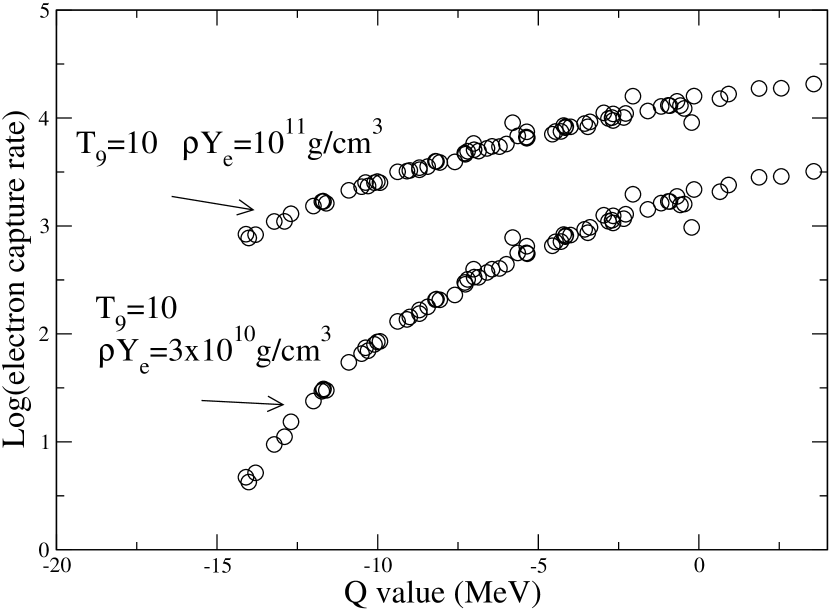
Figure 14: Electron capture rates for nuclei in the mass range A$<65\leq 80$ and for which (N-Z)/A$>$0.1 as a function of the Q-value (defined here as the parent daughter atomic mass difference). These rates have a simple dependence on the Q-value (see Eq. 26) because of our assumption that the configuration mixing strength is nucleus-independent for $GT^{+}$ blocked nuclei.

With the assumption that the high density electron capture rates are dominated by transitions involving low-lying configuration mixing strength, these rates are trivial functions of the electron Fermi energy and the parent-daughter mass difference. This is shown in figure 14 where the electron capture rates are presented for all nuclei with (N-Z)/A$>$0.1 that fall in the mass range A$=$66-80. The dependence of the rate on the Q-value for the transition is given by the simple analytic expression

$$\lambda\approx 2\ln(2)10^{-3.6}|M_{\rm GT}|^{2}({\rm F}_{4}(\eta_{\rm eff})+\bar{q}^{2}{\rm F}_{2}(\eta_{\rm eff})+2\bar{q}{\rm F}_{3}(\eta_{\rm eff})).$$ (26)

Here $\eta_{\rm eff}=(U_{\rm F}+m_{e}+q-E_{\rm res,d})/T$, with $E_{\rm res,d}$ the centroid of the ${\rm GT^{+}}$ resonance in the daughter, $\bar{q}=|q-E_{\rm res,d}|/T$, and the extra prefactor of 2 approximately accounts for the Coulomb distortion of the incoming electron for nuclei with $Z\approx 30-40$. This equation assumes that $q-E_{\rm res,d}$ is negative. The functions

$${\rm F_{k}(\eta)}=\int_{0}^{\infty}{x^{k}dx\over e^{x-\eta}+1}$$ (27)

appearing in Eq. 26 are the relativistic fermi integrals. Setting $E_{\rm res,d}=2{\,\rm MeV}$ and $|M_{\rm GT}|^{2}=1$ in Eq. 26 gives a reasonable estimate of the electron capture rates (when the rates are appreciable) when $U_{\rm F}>10\,{\rm MeV}$. These expressions can be used in place of our rate tables under these conditions. Using the simple approximations to the fermi functions developed in Fuller, Fowler and Newman (1985) gives an analytic approximation to the high density electron capture rates that is accurate to within the uncertainty in these rates. Electron capture rates for neutron rich nuclei at high electron fermi energies are essentially a function of only 1 parameter, the total $GT^{+}$ strength within a few MeV of the daughter state. Discrepancies between our calculated rates and more detailed calculations, e.g. monte carlo+RPA calculations (Langanke, Kolbe, & Dean, 2001), reflect the difference between our adopted $|M_{\rm GT}|^{2}=1$ and the more detailed estimate of $M_{\rm GT}$.

Fig. 14 also gives an estimate of the uncertainties in the electron capture rates. At $T_{9}=10$, $\rho Y_{e}=3\cdot 10^{10}{\rm g/cm^{3}}$ (${\rm U_{f}\approx 16\,MeV}$), an error of 2 MeV in the position of the centroid of the strength results in a change in the rate by a factor of $\sim 4$ for the nuclei with the smallest rates, and a factor of $\sim 2$ for the nuclei with the largest rates. At $T_{9}=10$, $\rho Y_{e}=10^{11}{\rm g/cm^{3}}$ (${\rm U_{f}\approx 23\,MeV}$), the uncertainty in the placement of the centroid implies an error of at most a factor of two in the electron capture rate. The uncertainty in the total strength is probably about a factor of 2 on average.

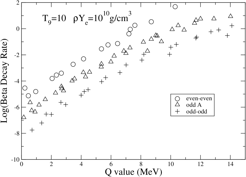
Figure 15: $\beta$ decay rates for neutron rich nuclei in the mass range A$<65\leq 80$ at $T_{9}=10$ and $\rho Y_{e}={10^{10}}{\rm g/cm^{3}}$. The systematics illustrated here are discussed in the text.

The systematics of the $\beta$ decay rates at high temperature and density are also simple. In Fig. 15 we show the $\beta$ decay rates at $T_{9}=10$, $\rho Y_{e}=10^{10}{\rm g/cm^{3}}$ for all nuclei with ${\rm(N-Z/A)>0.1}$. These rates fall into three distinct bands corresponding to odd-odd nuclei, even-even nuclei, and even-odd/odd-even nuclei. This can be understood by noting that at $T_{9}=10$ the ${\rm GT^{+}}$ resonance is thermally populated (under our assumption that the strength is centered at 2 MeV for these blocked nuclei). In this case the rate of decay is approximately $\lambda({\rm Q})Z_{\rm daughter}/Z_{\rm parent}$, where $\lambda({\rm Q})$ has a simple dependence on the Q-value. For even-even parents, $Z_{\rm daughter}/Z_{\rm parent}$ is typically approximately 20 at $T_{9}=10$, for odd-odd parents the ratio is about $1/20$, and for odd-even/even-odd parents the ratio of partition functions is about 1. Note that the $\beta$ decay rates are more sensitive to the (unknown) details of the strength distribution than the electron capture rates. At $T_{9}=10$, an error in the placement of the centroid of the resonance of 2 MeV changes the beta decay rate by about an order of magnitude.

6.4 Discussion and Conclusions

We have provided estimates of weak interaction rates for nuclei in the mass range A=65-80. These may be useful in simulations of x-ray bursts and pre-supernova stellar evolution. The rates have been calculated using available experimental information and simple estimates for the strength distributions and matrix elements for allowed and discrete-state transitions. The efficacy of our approach is confirmed through comparisons with detailed shell model based rates for nuclei in the mass range 60-65.

The single most uncertain aspect of the rate calculations is the ${\rm GT^{+}}$ resonance strength distribution. Our simple prescription gives good overall agreement with detailed shell model calculations of the ${\rm GT^{+}}$ strength for nuclei with A$\leq$65. However, our prescription is probably not reliable for nuclei at the end of the fp shell. Fortunately, nature to some extent does not seem to care about some of the hard to get details of the strength distribution for these nuclei. In the pre-collapse supernova this is because the nuclei present are nearly blocked to $GT^{+}$ transitions. (n,p) exchange experiments on such nuclei show that the strength is broad and low lying in the daughter. Because the electron fermi energies are high in the dense pre-supernova Fe-core, this implies that the electron capture rate is principally a function of the experimentally-determined parent-daughter mass difference. However, our work does not provide the detailed estimates of the magnitude of the configuration mixing strength that will ultimately also be needed for supernova simulations. The $\beta$ decay rates for the nuclei present in the late-time pre-supernova core are exponentially sensitive to the centroid energy of the ${\rm GT^{+}}$ resonance and are less certain. In x-ray burst environments the opposite condition holds: the parent daughter mass differences are typically large compared to the electron energies, so that the decay rate is dominated by the experimentally-determined lifetime.

The proper treatment of the high temperature electron capture and particulary beta decay rates is a challenging and important issue. Special care is needed in evaluating the partition functions for these rates. The beta decay rates for nuclei in these conditions is determined, among other things, by the nuclear partition function. In turn, the equilibrium nuclear composition is determined by the competition between beta decay and electron capture. If the partition functions used to estimate the composition at a given $Y_{e}$ do not match with the partition functions used to calculate the weak rates, the calculated equilibrium of the sytem will not be correct.

Table 1: Comparison of the shell model ${\rm GT^{-}}$ centroids calculated in Langanke (LMP) with those estimated from Eq. 20 (Present). All energies are in MeV and refer to energy with respect to the daughter ground state.

Parent Nucleus	LMP	Present
55Fe	12.6	10.4
56Fe	9.6	8.5
57Fe	12.6	11.5
58Fe	11.0	9.5
59Fe	13.6	12.6
60Fe	10.3	10.6
61Fe	13.8	13.75
62Fe	11.8	11.7
58Ni	9.2	6.44
59Ni	10.6	9.46
60Ni	9.0	7.5
61Ni	13.3	10.6
62Ni	9.2	8.2
63Ni	13.2	11.5
64Ni	9.6	9.15
65Ni	12.	12.35
56Co	13.2	12.7
57Co	12.5	10.77
58Co	14.7	13.7
59Co	13.1	11.6
60Co	14.0	14.8
61Co	13.6	12.6
62Co	15.3	13.9
63Co	14.4	13.7
64Co	16.0	16.7
65Co	14.6	14.8
55Mn	13.0	11.8
56Mn	14.7	15.1
57Mn	13.1	13.5
58Mn	15.5	16.4
59Mn	14.0	14.7
60Mn	16.0	17.4
61Mn	16.2	15.5

Note. — The shell model centroids in this table were taken from the tables or estimated from the graphs in Caurier et al. 1999 and LMP.

Table 2: Comparison of the shell model ${\rm GT^{+}}$ centroids calculated by LMP with those estimated from Eq. 21 (Present). All energies are in MeV and refer to energy with respect to the daughter ground state.

Parent Nucleus	LMP	Present
55Mn	4.6	4.6
56Mn	5.9	6.4
56Fe	2.6	2.4
56Co	8.2	8.8
58Mn	5.5	5.15
58Co	7.35	8.1
58Ni	3.75	3.65
59Co	5.05	5.0
60Co	6.35	6.74
60Ni	3.4	2.7
61Fe	2.1	1.8
61Co	3.7	3.4
61Ni	4.7	4.7
61Cu	6.7	6.4
62Ni	2.1	1.8
64Ni	1.3	1.8

Note. — The shell model centroids in this table were also taken from Caurier et al. 1999 and LMP. Where an experimental result is listed along with the shell model result we have presented the experimental result.

References

- Aufderheide et al. (1990) Aufderheide, M. B., Brown, G. E., Kuo, T. T. S., Stout, D. B. and Vogel, P. 1990, ApJ, 362, 241.
- Aufderheide et al. (1994) Aufderhide, M. B., Fushiki, I., Woosley, S. E., and Hartmann, D. H. 1994, ApJS, 91, 389.
- Aufderhide et al. (1996) Aufderhide, M. B., Bloom, S. D., Mathews, G. J., and Resler, D. A. 1996, Phys. Rev. C, 53, 3139.
- Bertsch and Esbensen (1987) Bertsch, G. F. and Esbensen, H. 1987, Reports on Progress in Physics, 50, 607.
- Bethe et al. (1979) Bethe, H. A., Brown, G. E., Applegate, J., and Lattimer, J. M. 1979, Nucl. Phys. A, 324, 487.
- Caurier et al. (1999) Caurier, E., Langanke, K., Martinez-Pinedo, G., and Nowacki, F. 1999, Nucl. Phys. A, 653, 439.
- Cooperstein and Wambach (1984) Cooperstein, J., and Wambach, J. 1984, Nucl. Phys. A, 420, 591.
- Fuller, Fowler and Newman (1980) Fuller G. M., Fowler, W. A. and Newman, M. J. 1980, ApJS, 42, 447 (FFNI).
- Fuller (1982) Fuller, G. M. 1982,ApJ, 252, 741.
- Fuller, Fowler and Newman (1982) Fuller G. M., Fowler, W. A. and Newman, M. J. 1982, ApJ, 252, 715 (FFNII).
- Fuller, Fowler and Newman (1982b) Fuller G. M., Fowler, W. A. and Newman, M. J. 1982, ApJS, 48, 279.
- Fuller, Fowler and Newman (1985) Fuller G. M., Fowler, W. A. and Newman, M. J. 1985, ApJ, 293, 1.
- Gaarde et al. (1981) Gaarde et al. 1981, Nucl. Phys. A, 369, 258.
- Helmer et al. (1997) Helmer, R. L. et al. 1997, Phys. Rev. C, 55, 2802.
- Hillman and Grover (1969) Hillman, M. and Grover, J. R. 1969, 185, 1303.
- Langanke, Kolbe, & Dean (2001) Langanke, K., Kolbe, E., & Dean, E. J. 2001, Phys. Rev. C, 63, 032801.
- Langanke and Martinez-Pinedo (2000) Langanke, K. and Martinez-Pinedo, G. 2001, Nucl. Phys. A, 673, 481.
- Rauscher and Thielemann (1999) Rauscher, T. and Thielemann, F. K. 2000, Atomic Data and Nuclear Data Tables, 75, 1.
- Rowe (1970) Rowe, J. 1970 in Nuclear Collective Motion, Models and Theory, Methuen, London.
- Sarriguren et al. (2001) Sarriguren, P., de Guerra, E. M., Escuderos, A. 2001, Nucl. Phys. A, 691, 631.
- Schatz et al. (1998) Schatz, H. et al. 1998, Phys. Rep., 294, 167.
- Schatz et al. (2001) Schatz, H. et al. 2001, Phys. Rev. Lett., 86, 3471.
- Vetterli et al. (1992) Vetterli, M. C. et al. 1992, Phys. Rev. C, 45, 997.
- Wallace and Woosley (1981) Wallace, R. K. and Woosley, S. E. 1981, ApJS, 45, 389.