Internal structure of a thin transonic disk

Abstract

The internal structure of the thin transonic disk accreting onto a nonrotating black hole inside the last stable orbit ($r<3r_{\rm g}$) is considered within the hydrodynamical version of the Grad-Shafranov equation. It is shown that in the vicinity of the sonic surface takes place a sharp diminishing of the disk thickness. As a result, in the vertical balance equation the dynamical forces $\rho[({\bf v}\nabla){\bf v}]_{\theta}$ become important, these on the sonic surface being of the same order as the pressure gradient $\nabla_{\theta}P$. In the supersonic region the thickness of the disk is determined by the form of ballistic trajectories rather than by the pressure gradient.

1 Introduction

According to the standard disk model [1], the matter forms a thin balanced disk and performs a circular motion with keplerian velocity $v_{\rm K}(r)=\left(G{\cal M}/r\right)^{1/2}$. The disk is thin provided that the accreting gas temperature is sufficiently low ($c_{\rm s}\ll v_{\rm K}$), so that $H\approx rc_{\rm s}/v_{\rm K}.$ Introducing the viscosity parameter $\alpha_{\rm SS}\leq 1$, relating the stress tensor $t_{\varphi}^{r}$ and the pressure as $t^{r}_{\varphi}=\alpha_{\rm SS}P$ [1], one can obtain

$$v_{r}/v_{\rm K}\approx\alpha_{\rm SS}\,c_{\rm s}^{2}/v_{\rm K}^{2}.$$ (1)

General relativity effects result in two important properties: the absence of stable circular orbits at small radii ($r<3r_{\rm g}$ for a nonrotating black hole, $r_{\rm g}=2G{\cal M}/c^{2}$ is the gravitational radius), and the transonic regime of accretion. The former means that for $r<3r_{\rm g}$ a flow can be realized in the absence of viscosity. The latter results from the fact that according to (1) the flow is subsonic outside the marginally stable orbit $r=3r_{\rm g}$ while at the horizon $r=r_{\rm g}$ the flow is to be supersonic.

Up to now in the majority of works the procedure of vertical averaging was used, where vertical four-velocity $u_{\hat{\theta}}$ was assumed to be small [2, 3]. As a result, the vertical component of the dynamic force $nu^{b}\nabla_{b}(\mu u_{\hat{\theta}})$ was postulated to be unimportant up to horizon. Here we are going to demonstrate that the assumption $u_{\hat{\theta}}=0$ is not correct. As in the Bondi accretion, the dynamic force is to be important in the vicinity of the sonic surface.

2 Basic equations

Consider ideal gas accreting onto a black hole inside the marginally stable orbit $r=3r_{\rm g}$. Exact equations of motion of ideal media in Kerr metric were formulated in [4]. We consider a non-rotating (Schwarzschild) black hole only.

In Boyer-Lindquist coordinates ($t,r,\theta,\varphi$) the Schwarzschild metric is [1] ${\rm d}s^{2}=-\alpha^{2}{\rm d}t^{2}+g_{ik}{\rm d}x^{i}{\rm d}x^{k},$ where $\alpha^{2}=1-2{\cal M}/r,\,g_{rr}=\alpha^{-2},\,g_{\theta\theta}=r^{2}$, and $g_{\varphi\varphi}=\varpi^{2}=r^{2}\sin^{2}\theta.$ Here indices without caps denote vector components with respect to the coordinate basis $\partial/\partial r$, $\partial/\partial\theta$, $\partial/\partial\varphi$ and indices with caps denote their physical components. The ${\bf\nabla}_{k}$ symbol always represents a covariant derivative in space with $g_{ik}$ metric. Finally, below we always use a system of units with $c=G=1$.

It is convenient to introduce a stream function $\Phi(r,\theta)$. This function defines the physical poloidal four-velocity component ${\bf u}_{\rm p}$ as

$$\alpha n{\bf u}_{\rm p}=\frac{1}{2\pi\varpi}({\bf\nabla}\Phi\times{\bf e}_{\hat{\varphi}}).$$ (2)

Here $n$ is the particle concentration in the comoving reference frame. It is the curves $\Phi(r,\theta)=$ const that define lines of flow of the matter.

Three integrals of motion are conserved on $\Phi(r,\theta)=$ const surfaces: entropy $S=S(\Phi)$, energy $E(\Phi)$, and $z$-component of angular momentum $L(\Phi)$

$$E(\Phi)=\mu\alpha\gamma,\qquad L(\Phi)=\mu\varpi u_{\hat{\varphi}}.$$ (3)

Here $\mu=(\rho_{m}+P)/n$ ($\rho_{m}$ is internal energy density) is the relativistic enthalpy. Below for simplicity we use the polytropic equation of state $P=k(S)n^{\Gamma}$, so that the temperature and the sound velocity can be written as [1]

$$T=k(S)n^{\Gamma-1},\qquad c_{\rm s}^{2}=\frac{\Gamma}{\mu}k(S)n^{\Gamma-1}.$$ (4)

As a result, the relativistic Euler equation

$$nu^{b}\nabla_{b}(\mu u_{a})+\nabla_{a}P-\mu n(u_{\hat{\varphi}})^{2}\frac{1}{\varpi}\nabla_{a}\varpi+\mu n\gamma^{2}\frac{1}{\alpha}\nabla_{a}\alpha=0$$ (5)

can be rewritten in the form of the Grad-Shafranov scalar equation for the stream function $\Phi(r,\theta)$ containing three integrals $E(\Phi)$, $L(\Phi)$, and $S(\Phi)$ [4]

$$-M^{2}\left[\frac{1}{\alpha}\nabla_{k}\left(\frac{1}{\alpha\varpi^{2}}\nabla^{k}\Phi\right)+\frac{1}{\alpha^{2}\varpi^{2}(\nabla\Phi)^{2}}\frac{\nabla^{i}\Phi\nabla^{k}\Phi\nabla_{i}\nabla_{k}\Phi}{D}\right]$$

(6)

$$+\frac{M^{2}\nabla^{\prime}_{k}F\nabla^{k}\Phi}{2\alpha^{2}\varpi^{2}({\bf\nabla}\Phi)^{2}D}+\frac{64\pi^{4}}{\alpha^{2}\varpi^{2}M^{2}}\left(\varpi^{2}E\frac{{\rm d}E}{{\rm d}\Phi}-\alpha^{2}L\frac{{\rm d}L}{{\rm d}\Phi}\right)-16\pi^{3}nT\frac{{\rm d}S}{{\rm d}\Phi}=0,$$

in which the $\nabla^{\prime}_{k}$ derivative acts on all the variables except the quantity $M^{2}$. Here the thermodynamical function $M^{2}$ is defined as $M^{2}=4\pi\mu/n$ and

$$D=-1+\frac{1}{u^{2}_{\rm p}}\frac{c^{2}_{s}}{1-c^{2}_{s}},\quad F=\frac{64\pi^{4}}{M^{4}}\left[\varpi^{2}E^{2}-\alpha^{2}L^{2}-\varpi^{2}\alpha^{2}\mu^{2}\right].$$ (7)

To make the system complete we need to supply Grad-Shafranov equation (6) with the relativistic Bernoulli equation $u_{\rm p}^{2}=\gamma^{2}-u_{\hat{\varphi}}^{2}-1$; the latter with the help of (3) can be rewritten as follows:

$$u_{\rm p}^{2}=(E^{2}-\alpha^{2}L^{2}/\varpi^{2}-\alpha^{2}\mu^{2})/\alpha^{2}\mu^{2}.$$ (8)

3 Subsonic flow

First of all, let us consider the subsonic region in the very vicinity of the marginally stable orbit $r=r_{0}=3r_{\rm g}$ where the poloidal velocity is much smaller than that of sound. Then equation (6) can be significantly simplified by neglecting the terms proportional to $D^{-1}\sim u_{\rm p}^{2}/c_{\rm s}^{2}$. As a result, we have

$$-\frac{M^{2}}{\alpha}\nabla_{k}\left(\frac{\nabla^{k}\Phi}{\alpha\varpi^{2}}\right)+\frac{64\pi^{4}}{\alpha^{2}\varpi^{2}M^{2}}\left(\varpi^{2}E\frac{{\rm d}E}{{\rm d}\Phi}-\alpha^{2}L\frac{{\rm d}L}{{\rm d}\Phi}\right)-16\pi^{3}nT\frac{{\rm d}S}{{\rm d}\Phi}=0.$$ (9)

This equation describing the subsonic flow is elliptical. Hence, it is necessary to specify five boundary conditions on the surface of the last stable orbit $r_{0}=3r_{\rm g}$ where $\alpha_{0}=\alpha(r_{0})=\sqrt{2/3}$, $u_{\hat{\varphi}}(r_{0})=1/\sqrt{3}$, and $\gamma_{0}=\gamma(r_{0})=\sqrt{4/3}$ [1]. We consider below the case where the radial velocity is constant on the surface $r=r_{0}$ and the toroidal four-velocity is exactly equal to $u_{\hat{\varphi}}(r_{0})$:

$$u_{\hat{r}}(r_{0},\Theta)=-u_{0},\quad u_{\hat{\Theta}}(r_{0},\Theta)=\Theta u_{0},\quad u_{\hat{\varphi}}(r_{0},\Theta)=1/\sqrt{3}.$$ (10)

Here $u_{\hat{\Theta}}\left(r_{0},\Theta\right)$ corresponds to the plane flow at the marginally stable orbit, and we introduced the new angular variable $\Theta=\pi/2-\theta$ ($\Theta_{\rm disk}\sim c_{0}$) which is counted off from the equator in the vertical direction. Next, we suppose that the velocity of sound is also a constant on the surface $r=r_{0}$:

$$c_{\rm s}(r_{0},\Theta)=c_{0}.$$ (11)

For $P=k(S)n^{\Gamma}$ this means that both the temperature $T_{0}=T(r_{0})$ and the relativistic enthalpy $\mu_{0}=\mu(r_{0})$ are also constant on this surface. It is necessary to stress that, according to (1), for nonrelativistic temperature of the accreting gas $c_{0}\ll 1$ we have a small parameter $u_{0}/c_{0}\sim\alpha_{\rm SS}c_{0}\ll 1$. Finally, as the last, fifth, boundary condition it is convenient to specify the entropy $S(\Phi)$.

Introducing now the values $e_{0}=\alpha_{0}\gamma_{0}=\sqrt{8/9}$ and $l_{0}=u_{\hat{\varphi}}(r_{0})r_{0}=\sqrt{3}r_{\rm g}$, one can rewrite the invariants $E(\Phi)$ and $L(\Phi)$ as

$$E(\Phi)=\mu_{0}e_{0}={\rm const},\qquad L(\Phi)=\mu_{0}l_{0}\cos\Theta_{m}.$$ (12)

Here $\Theta_{m}=\Theta_{m}(\Phi)$ is the angle for which $\Phi(r_{0},\Theta_{m})=\Phi(r,\Theta)$. In other words, the function $\Theta_{m}(r,\Theta)$ has the meaning of a theta angle on the last stable orbit connected with a given point ($r$,$\Theta$) by a line of flow $\Phi(r,\Theta)=$ const. In particular, $\Theta_{m}(r_{0},\Theta)=\Theta$.

First of all, we see that condition $E=$ const (12) allows us to rewrite equation (9) in a simpler form

$$\frac{\partial^{2}\Phi}{\partial r^{2}}+\frac{\cos\Theta}{\alpha^{2}r^{2}}\frac{\partial}{\partial\Theta}\left(\frac{1}{\cos\Theta}\frac{\partial\Phi}{\partial\Theta}\right)=-4\pi^{2}n^{2}\frac{L}{\mu^{2}}\,\frac{{\rm d}L}{{\rm d}\Phi}-4\pi^{2}n^{2}r^{2}\cos^{2}\Theta\frac{T}{\mu}\,\frac{{\rm d}S}{{\rm d}\Phi}.$$ (13)

Next, as one can show [5], for $r=r_{0}$, the r.h.s. of equation (13) describes the transverse balance of a pressure gradient and a gravitational force, whereas the l.h.s. corresponds to the dynamic term $({\bf v}\nabla){\bf v}$. At the marginally stable orbit it is of the order of $u_{0}^{2}/c_{0}^{2}$ and may be dropped. It is therefore natural to choose the entropy $S(\Phi)$ from the condition of a transverse balance on the surface $r=r_{0}$

$$r_{0}^{2}\cos^{2}\Theta_{m}\frac{{\rm d}S}{{\rm d}\Theta_{m}}=-\frac{\Gamma}{c_{0}^{2}}\,\frac{L}{\mu_{0}^{2}}\,\frac{{\rm d}L}{{\rm d}\Theta_{m}},$$ (14)

where $L(\Theta_{m})$ is determined from the boundary condition (12). Thus, we have

$$S(\Theta_{m})=S(0)-\frac{\Gamma}{3c_{0}^{2}}\ln(\cos\Theta_{m}).$$ (15)

Owing to (11), relation (15) corresponds to the standard concentration profile

$$n(r_{0},\Theta)\approx n_{0}\exp\left(-\frac{\Gamma}{6c_{0}^{2}}\Theta^{2}\right).$$ (16)

Finally, definition (2) results in the following relationship between functions $\Phi$ and $\Theta_{m}$:

$${\rm d}\Phi=2\pi\alpha_{0}r_{0}^{2}n(r_{0},\Theta_{m})u_{0}\cos\Theta_{m}{\rm d}\Theta_{m}.$$ (17)

Hence, due to (12), (16), and (17), the invariant $L(\Phi)$ can be directly determined from the boundary conditions as well.

Equation (13) together with boundary conditions (10), (12), (15), (16), and (17) determines structure of the inviscid subsonic flow inside the marginally stable orbit. For example, for $c_{\rm s}\ll 1$ we obtain using (8)

$$u_{\rm p}^{2}=u_{0}^{2}+w^{2}+\frac{1}{3}\left(\Theta_{m}^{2}-\Theta^{2}\right)+\frac{2}{\Gamma-1}(c_{0}^{2}-c_{\rm s}^{2})+\dots$$ (18)

Here the quantity $w$, where

$$w^{2}(r)=\frac{e_{0}^{2}-\alpha^{2}l_{0}^{2}/r^{2}-\alpha^{2}}{\alpha^{2}}\approx\frac{1}{6}\,\left(\frac{r_{0}-r}{r_{0}}\right)^{3},$$ (19)

depending on the radius $r$ only, is a poloidal four-velocity of a free particle having zero poloidal velocity for $r=r_{0}$. As we see, $w^{2}$ increases very slowly when moving away from the last stable orbit. Therefore, the contribution of $w^{2}$ turns out to be negligibly small in the subsonic region.

An important conclusion can be drawn directly from (18) in which for the equatorial plane we have $\Theta_{m}=\Theta=0.$ Assuming $u_{\rm p}=c_{\rm s}=c_{*}$ and neglecting $w^{2}$, we find the velocity of sound $c_{*}$ on the sonic surface $r=r_{*}$, $\Theta=0$:

$$c_{*}\approx\sqrt{\frac{2}{\Gamma+1}}\,c_{0}.$$ (20)

As we see, $c_{*}\approx c_{0}$. Next, as the entropy $S$ remains constant along the flow lines, the gas concentration remains approximately constant along the flow lines ($n(r_{*},\Theta)\approx n(r_{0},\Theta_{m})$) as well. In other words, in agreement with the Bondi accretion, the subsonic flow can be considered incompressible. On the other hand, because the radial velocity increases from $u_{0}$ to $c_{*}\approx c_{0}$, i.e., for $c_{0}\ll 1$ ($u_{0}/c_{0}\ll 1$) it changes over several orders of magnitude, the disk thickness $H$ should change in the same proportion owing to the continuity equation (see Fig. 1)

$$H(r_{*})\approx\frac{u_{0}}{c_{0}}H(r_{0}).$$ (21)

As a result, a rapid decrease of the disk thickness should be accompanied by the appearance of vertical component of velocity which also should be taken into account in Euler equation (5).

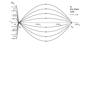
Figure 1: The structure of a thin accretion disk (actual scale) for $c_{0}=10^{-2}$, $u_{0}=10^{-5}$ after passing the marginally stable orbit $r=3r_{\rm g}$. In the vicinity of the sonic surface $r=r_{*}$ the flow has a form of an ordinary nozzle.

Indeed, as one can find analyzing asymptotic of equation (13) [5], in the vicinity of the sonic surface located at $r_{*}=r_{0}-\Lambda u_{0}^{2/3}r_{0}$, where the logarithmic factor $\Lambda=(3/2)^{2/3}[\ln(c_{0}/u_{0})]^{2/3}\approx 5-7$, the components of the velocity and the pressure gradient in the limit $r\rightarrow r_{*}$ can be presented as

$$u_{\hat{\Theta}}\rightarrow-\frac{c_{0}}{u_{0}}\Theta,\quad u_{\hat{r}}\rightarrow-c_{*},\quad-\frac{\nabla_{\hat{\Theta}}P}{\mu}\rightarrow\frac{c_{0}^{2}}{u_{0}^{2}}\,\frac{\Theta}{r}.$$ (22)

On the other hand, near the sonic surface the radial scale $\delta r$ determining the radial derivatives becomes as small as the transverse dimension of a disk: $\delta r\approx H(r_{*})\approx u_{0}r_{0}$. Hence, logarithmic derivative $\eta_{1}=(r/n)(\partial n/\partial r)$ can be evaluated as $\eta_{1}\approx u_{0}^{-1}$. As a result, both components of the dynamic force

$$\frac{u_{\hat{\Theta}}}{r}\,\frac{\partial u_{\hat{\Theta}}}{\partial\Theta}\rightarrow\frac{c_{0}^{2}}{u_{0}^{2}}\,\frac{\Theta}{r},\quad u_{\hat{r}}\frac{\partial u_{\hat{\Theta}}}{\partial r}\rightarrow\frac{c_{0}^{2}}{u_{0}^{2}}\,\frac{\Theta}{r},$$ (23)

do become of the order of the pressure gradient.

4 Transonic flow

To check our conclusion one can consider flow structure in the vicinity of the sonic surface in more detail. Because the smooth transonic flow is analytical at a singular point, one can write

$$n = n_{*}\left(1+\eta_{1}h+\frac{1}{2}\eta_{3}\Theta^{2}+\dots\right),$$ (24)

$$\Theta_{m} = a_{0}\left(\Theta+a_{1}h\Theta+\frac{1}{2}a_{2}h^{2}\Theta+\frac{1}{6}b_{0}\Theta^{3}+\dots\right),$$ (25)

where $h=(r-r_{*})/r_{*}$. Here we assume that all the three invariants $E$, $L$, and $S$ are already given. Hence, the problem needs one extra boundary condition. Now comparing the appropriate coefficients in Bernoulli (8) and full stream equation (6), one can obtain neglecting terms $\sim u_{0}^{2}/c_{0}^{2}$

$$a_{0} = \left(\frac{2}{\Gamma+1}\right)^{(\Gamma+1)/2(\Gamma-1)}\frac{c_{0}}{u_{0}},$$ (26)

$$a_{1} = 2+\frac{1-\alpha_{*}^{2}}{2\alpha_{*}^{2}}\approx 2.25,$$ (27)

$$a_{2} = -(\Gamma+1)\eta_{1}^{2},$$ (28)

$$b_{0} = \left(\frac{\Gamma+1}{6}\right)\frac{a_{0}^{2}}{c_{0}^{2}},$$ (29)

$$\eta_{3} = -\frac{2}{3}(\Gamma+1)\eta_{1}^{2}-\left(\frac{\Gamma-1}{3}\right)\frac{a_{0}^{2}}{c_{0}^{2}},$$ (30)

where $\alpha_{*}^{2}=\alpha^{2}(r_{*})\approx 2/3$.

As we see, coefficients (26)–(30) are expressed through the radial logarithmic derivative $\eta_{1}$. They have clear physical meaning. So, $a_{0}$ gives the compression of flow lines: $a_{0}=H(r_{0})/H(r_{*})$. In agreement with (21) we have $a_{0}\approx c_{0}/u_{0}$. Further, $a_{1}$ corresponds to the slope of the flow lines with respect to the equatorial plane. As $a_{1}>0$, the compression of stream line finishes somewhere before the sonic surface, so inside the sonic radius $r<r_{*}$ the stream lines diverge. On the other hand, as $a_{1}\ll u_{0}^{-1}$, for $r=r_{*}$ the divergency is still very weak. Hence, in the vicinity of the sonic surface the flow has a form of an ordinary nozzle (see Fig. 1). Finally, as $a_{2}\sim\eta_{3}\sim b_{0}\sim u_{0}^{-2}$, one can conclude that the transverse scale of the transonic region $H(r_{*})$ is the same as the longitudinal one. The latter point suggests a very important consequence that the transonic region is essentially two-dimensional, and it is impossible to analyze it within the standard one-dimensional approximation.

Let us stress that it is rather difficult to connect the sonic characteristics $\eta_{1}=\eta_{1}(r_{*})$ with physical boundary conditions on the marginally stable orbit $r=r_{0}$ (for this it is necessary to know all the expansion coefficients in (24) and (25)). In particular, it is impossible to formulate the restriction on five boundary conditions (10), (11) and (15) resulting from the critical condition on the sonic surface. Nevertheless, the estimate $\eta_{1}\approx u_{0}^{-1}$ makes us sure that we know the parameter $\eta_{1}$ to a high enough accuracy. Then, according to (26)–(30), all the other coefficients can be determined exactly.

Using now expansions (24) and (25), one can obtain all other physical parameters of the transonic flow. In particular, we have

$$u_{\rm p}^{2} = c_{*}^{2}\left[1-2\eta_{1}h+\frac{1}{6}(\Gamma-1)\,\frac{a_{0}^{2}}{c_{0}^{2}}\Theta^{2}+\frac{2}{3}(\Gamma+1)\eta_{1}^{2}\Theta^{2}\right],$$

$$c_{\rm s}^{2} = c_{*}^{2}\left[1+\left(\Gamma-1\right)\eta_{1}h+\frac{1}{6}(\Gamma-1)\,\frac{a_{0}^{2}}{c_{0}^{2}}\Theta^{2}-\frac{1}{3}(\Gamma-1)(\Gamma+1)\eta_{1}^{2}\Theta^{2}\right].$$

Hence, a shape of the sonic surface $u_{\rm p}=c_{\rm s}$ has the standard parabolic form

$$h=\frac{1}{3}\eta_{1}\Theta^{2}.$$ (31)

5 Supersonic flow

Because the pressure gradient becomes insignificant in supersonic region, the matter moves here along the trajectories of free particles. Neglecting $\nabla_{\theta}P$ term in the $\theta$-component of relativistic Euler equation (5), we have (cf. [3])

$$\alpha u_{\hat{r}}\frac{\partial(ru_{\hat{\Theta}})}{\partial r}+{(ru_{\hat{\Theta}})\over r^{2}}\frac{\partial(ru_{\hat{\Theta}})}{\partial\Theta}+(u_{\hat{\varphi}})^{2}\tan\Theta=0.$$ (32)

Here $u_{\hat{\varphi}}$ can be easily expressed in terms of radius: $u_{\hat{\varphi}}=\sqrt{3}/x,$ where $x=r/r_{\rm g}$. We also introduce dimensionless functions $f(x)$ and $g(x)$: $\Theta f(x)=xu_{\hat{\Theta}}$, $g(x)=-\alpha u_{\hat{r}}>0$. Using now (32) and definitions above, we obtain an ordinary differential equation for $f(x)$

$$\frac{{\rm d}f}{{\rm d}x}=\frac{f^{2}+3}{x^{2}g(x)}.$$ (33)

Next, analyzing equation (8), one can conclude that $u_{\rm p}\rightarrow w$ as $r\rightarrow r_{\rm g}$. On the other hand, $u_{\rm p}\approx c_{*}\approx c_{0}$ for $r\lesssim r_{*}$. Therefore, the following approximation should be valid throughout $r_{\rm g}<r<r_{*}$ region: $g(x)\approx\sqrt{(\alpha w)^{2}+(\alpha c_{0})^{2}}$, where, owing to (19), $\left(\alpha w\right)^{2}=(3-x)^{3}/(9x^{3})$.

The results of calculations are presented on Fig. 1. As we see, in the supersonic region the flow performs transversal oscillation about the equatorial plane, their frequency independent of the amplitude. Once diverged, the flow converges once again at the point $r=r_{\rm cr}$ ($r_{0}-r_{\rm cr}=Ac_{*}r_{0}$, $A\approx 2\pi$) on the equatorial plane. Such oscillation can be easily understood. Indeed, as one can see from (18), for $c_{0}\ll 1$ poloidal motion remains nonrelativistic for $r\sim r_{*}$. Hence, it is possible to use the nonrelativistic equation

$$\frac{{\rm d}v_{\hat{\Theta}}}{{\rm d}t}=-\Theta\frac{v_{\hat{\varphi}}^{2}}{r},$$ (34)

where $v_{\hat{\Theta}}=r{\rm d}\Theta/{\rm d}t$. Because the spatial amplitude of oscillations $\sim c_{0}r_{0}$ is small compared with $r_{0}$, one can write $v_{\hat{\varphi}}=u_{\hat{\varphi}}(r_{0})/\gamma_{0}=1/2$ (see (10)), $r=3r_{\rm g}$, and $|v_{r}|\approx c_{*}$. This gives $\Theta(h)=\Theta_{\rm A}\sin[(v_{\hat{\varphi}}/c_{*})h]$, $h=(r-r_{*})/r_{*}$ in full agreement with exact calculations. Clearly, additional consideration is necessary to determine the flow structure for $r<r_{\rm cr}$. Nevertheless, one can be sure that the accretion disk thickness, though oscillating in the supersonic region, remains as small as in the region of stable orbits: $\Theta_{\rm disk}\lesssim c_{0}$.

6 Conclusion

As was shown, the diminishing disk thickness in the vicinity of the sonic surface inevitably leads to the emergence of the vertical velocity component of the accreting matter. As a result, the dynamic term $({\bf v}\nabla){\bf v}$ in the vertical balance equation cannot be omitted. It is necessary to stress that whereas at the sonic surface both components of dynamic term $[({\bf v}\nabla){\bf v}]_{\theta}$ (23) become of the same order of magnitude as the pressure gradient, the role of the gravitational term remains unimportant: $\nabla_{\theta}\varphi_{\rm g}\sim\Theta/r$, i.e., it is $c_{0}^{2}/u_{0}^{2}$ times smaller than the leading terms. As a result, the structure of a thin transonic disk is quite similar to that of an ordinary planar nozzle. For this reason the critical condition on the sonic surface does not restrict the accretion rate. We suppose that for a given accretion rate it determines vertical component of the velocity on the marginally stable orbit which does not affect the flow structure. Finally, inside the sonic surface $r<r_{*}$ the pressure term $\nabla_{\theta}P$ becomes unimportant, so the thickness of the disk is determined by the form of ballistic trajectories.

This work was partially supported by the Russian Foundation for Basic Research (grant No. 00–15–96594).

• [1] S.L. Shapiro and S.A. Teukolsky, Black Holes, White Dwarfs, and Neutron Stars, A Wiley–Interscience Publication, New York, 1983.
• [2] B. Paczynski and G.S. Bisnovatyi-Kogan, Acta Astron. 31 (1981) 283.
• [3] M.A. Abramowicz, A. Lanza, and M.J. Percival, Astrophys. J. 479 (1997) 179.
• [4] V.S. Beskin and V.I. Pariev, Physics Uspekhi 36 (1993) 529.
• [5] V.S. Beskin, R.Yu. Kompaneetz, and A.D. Tchekhovskoy, Astron. Lett. 28 (2002) 543.