“Fundamental-Plane”-Like Relations From Collisionless Stellar Dynamics: A Comparison of Mergers and Collapses

Abstract

We present a new set of dissipationless N-body simulations aiming to better understand the pure dynamical aspects of the “Fundamental Plane” (FP) of elliptical galaxies. We have extended our previous hierarchical merger scheme by considering the Hernquist profile for the initial galaxy model. Two-component Hernquist galaxy models were also used to study the effect of massive dark halos on the end-products characteristics. We have also performed new collapse simulations including initial spin. We found that the one-component Hernquist mergers give results similar to those found for the one-component King models, namely both were able to build-up small scatter FP-like correlations with slopes consistent with what is found for the near-infrared FP of nearby galaxies. The two-component models also reproduce a FP-like correlation, but with a significantly steeper slope. This is in agreement with what has been found for elliptical galaxies at higher redshift (0.1 $<$ z $<$ 0.6). We discuss some structural properties of the simulated galaxies and their ability to build-up FP-like correlations. We confirm that collapses generally do not follow a FP-like correlation regardless of the initial spin. We suggest that the evolution of gradients in the gravitational field of the merging galaxies may be the main ingredient dictating the final non-homology property of the end products.

1 Introduction

The origin of the “Fundamental Plane” relation (hereon FP) of elliptical galaxies is still unknown, despite of all the efforts to understand it since it was discovered (Djorgovski & Davis 1987, Dressler et al. 1987).

On fundamental grounds, the simplest version of the virial theorem applied to galaxies predicts that they should form a family of objects following a simple projected relation, involving structural and kinematical variables, for instance: $r_{e}=C_{vir}\sigma_{0}^{2}I_{e}^{-1}$. In this equation, $C_{vir}$ is a structural-kinematical parameter, $\sigma_{0}$ is the central projected velocity dispersion, $I_{e}$, the average surface brightness within the effective radius in linear units, and $r_{e}$ is the effective radius. The coefficient $C_{vir}$ relates physical (3-D) to projected variables, like the velocity dispersion and mass distributions. Hence, $C_{vir}\equiv C_{vir}(C_{r},C_{v},M/L)$ depends on kinematical ($C_{v}$) and structural ($C_{r}$) coefficients, as well as on the mass-luminosity ratio ($M/L$) of the systems (c.f. Capelato, de Carvalho & Carlberg 1995, hereon CdCC95; Dantas et al. 2001, hereon DCdCR01).

We define a family of homologous galaxies as virialized systems where the kinematical and structural coefficients are simply constant for all galaxies, or may change but in a constant ratio throughout the family. If furthermore $M/L$ is constant for all galaxies (or equivalently, $M$ and $L$ may change among them but in a constant ratio), then $C_{vir}$ is a constant for a given homologous family.

The expression of the FP is similar to that expected from the projected virial relation but with significantly different exponents and small scatter throughout: $r_{e}\sim\sigma_{0}^{A}I_{e}^{B}$ (where the exponents are: $A\sim 1.53$, $B\sim-0.79$, e.g. Pahre, Djorgovski & de Carvalho 1998). Thus, in the case of ellipticals, it is inferred that $C_{vir}$ must vary monotonically among these galaxies if one is willing to retrieve the virial relation for these systems.

There are several reasonable alternatives to explain why and how $C_{vir}$ should vary in order to explain the discrepancy between the virial theorem and the FP. One of them assumes a systematic variation of $M/L$ with the total mass of the system, preserving homology. This would be responsible for the whole $C_{vir}$ variation (e.g. Djorgovski 1988, Djogorvski & Santiago 1993, Renzini et al. 1993, Pahre & Djorgovski 1997). This dependence would be caused by systematic stellar population (e.g. mean stellar age, metallicity, etc.) variations with mass. Pahre & Djorgovski (1997) have shown that there is a dependence of the FP tilt with wavelength, namely $M/L\propto L^{\beta}$ where $\beta$ varies with the photometric band ($\lambda$) in which the luminosity is measured. This means that $\beta$ decreases from the $B$ to the $K$ band, although never reaching the homologous, virial expectations. As discussed by Pahre & Djorgovski, the trend of $\beta$ with $\lambda$ cannot be explained solely by either stellar population models or non-homology (see their Figure 2). They conclude that a more complete scenario to explain the FP tilt has to invoke contributions from both effects. Broken homology can be achieved both in dissipationless hierarchical merging scenarios (e.g., CdCC95) and in dissipative mergers of star-forming and gas-rich spirals, where the roles of star formation histories are emphasized (c.f. Bekki 1998). A third line of reasoning for explaining the FP assumes that a more refined formulation to describe the equilibrium condition of the luminous component of the elliptical galaxies is adopting a “two-component virial theorem”, which assumes of course that ellipticals are dynamically dominated by a dark halo (Dantas et al. 2000).

In the present work, we study the origin of the FP tilt under the assumption that elliptical galaxies are more closely described as non-homologous virialized systems, with $C_{v}$ and/or $C_{r}$ varying monotonically (e.g., CdCC95, Hjorth & Madsen 1995, Capelato, de Carvalho & Carlberg 1997,Ciotti, Lanzoni & Renzini 1996, Busarello et al. 1997, Graham & Colless 1997, Bekki 1998). In a hierarchical galaxy formation scenario, galaxies are built-up by sucessive merge of larger and larger systems. Recent observations have reinforced the idea of hierarchical merger as a reasonable mechanism to form elliptical galaxies (e.g. Bender & Saglia 1999), although dissipation seems to be an important ingredient. In any case, numerical investigations of merging seem to be fundamental in understanding the scaling relations of these objects. The numerical work of CdCC95 has shown, for instance, that the FP correlations can arise naturally from objects that are formed by dissipationless hierarchical mergers of galaxies. The end products of their simulations result in a non-homologous family of objects, being the peculiar non-homology mainly determined by the parameter $C_{v}$ varying systematically with the initial orbital energy of the galactic pairs. In a subsequent investigation, DCdCR01 have shown that one-component, equal mass collapses of several different initial models and collapse factors produce nearly homologous families of objects. This result led DCdCR01 to suggest that the driving mechanism producing non-homology would be that of merging per se.

We extend the previous dissipationless numerical investigations in several aspects. First, the equilibrium models considered by CdCC95 (King spheres) do not take into consideration a central density peak. Recent studies (e.g. Gerhardt et al. 2000, Siopis et al. 2000) have demonstrated, however, that the presence of a central peak (or even the presence of a central black hole) should be much more common in elliptical galaxies than previously thought. Here we consider the hierarchical merge of Hernquist models, which present a central density “cusp”. Second, CdCC95 only consider one component models. However, it is important to understand the effect of the halo in the dynamics of merging and the consequences of its influence in the equilibrium conditions of the whole system (Dantas et al. 2000). In this paper we consider the merge of two-component Hernquist models up to two generations.

One point not addressed by DCdCR01 was the initial difference in spin parameters between proto-galaxies and how that can introduce non-homology into the structural properties of the final objects. In order to address this point, we investigate how the spin parameter influences the FP of the collapsed objects. However, the issue which we leave for future work is the study of two-component collapses. This is an important problem, since in the currently accepted cosmological scenarios, the luminous component collapses in the dark matter halo already virialized some time after the epoch of equality of matter and radiation energy densities. Our present goal is to establish the behaviour of only one-component collapses before analysing two-component ones, which can be studied under a more general approach as, for instance, drawing the models from high resolution cosmological simulations.

This paper is organized in the following way: in Section 2, we present the simulation setups and initial condition grids; in Section 3, the end products of the simulations are considered in the context of the FP space and the resulting relaxation histories. Finally, in section 4, we discuss our main results.

2 Simulations Setup and Definition of Characteristic Parameters

2.1 Computer Plataforms and Codes

The simulations were run using two C translations (c.f. Dubinski 1988) of the TREECODE (Barnes & Hut 1986): a non-parallel version, which was used to run less CPU time consuming, one-component model simulations; and a parallel version, run for two-component model simulations. The computational plataforms used were: (i) For the non-parallel code: Workstations Sun-Sparc; Sun-Ultras (1, 2, 5, 10, and 30); and Sun E250; (ii) For the parallel code: Silicon Graphics Origin 2000 with four processors using MPI (“Message Passing Interface”), IRIX operational system; and a “cluster” formed by four Pentium III, 650 MHz, working in parallel using LAM (“Local Area Multicomputer”) 6.3.2/MPI 2 C++, Linux.

Quadrupole correction terms, according to Dubinski (1988), were used in the force calculations for all simulations. In Table 1 we list the main parameters of the simulations setup adopted in this work. These parameters were carefully chosen in order to conform to the constraints of resolution and collisionlessness given the total number of particles used in each type of simulation (more details for the choice of parameters can be found in CdCC95 and DCdCR01). In particular, the choice of the number of particles was also based on the operational constraints due to CPU times. Merging generaly involves CPU time-consuming runs for it includes the evolution since the initial orbital phase, before the effective merge of the systems. This forced us to use a relatively small number of particles to cover a wider grid of initial conditions. These numbers, however, are well above the lower bound discussed in DCdCR01.

Table 1: Initial Parameters of the Codes

Parameter	Value
$\theta$: tolerance	$0.8$
$\epsilon$: softening
$~{}~{}~{}\rightarrow$ Non-parallel code	$0.05$
$~{}~{}~{}\rightarrow$ Parallel code
Luminous component	$0.07$
Dark component	$0.7$
$\Delta t$: time integration step	$0.025$

2.2 Initial Condition Grid of the Models

2.2.1 Computational Units

The units used in our simulations were all set to match those of CdCC95 and DCdCR01: the mass and lenght units were set to $M_{U}\equiv 10^{10}$ $M_{\odot}$ and $L_{U}\equiv 1$ kpc, respectively. These values, and $G\equiv 1$, fix our time and velocity units to $T_{U}\equiv 4.72$ Myr and $v_{U}\equiv 207$ km s^-1, respectively.

2.2.2 The Merger Models

The initial equilibrium models for the merger pair were each obtained from $N$ particles random realizations of spheres in hydrostatic equilibrium, obeying the Hernquist profile (c.f. Hernquist 1990). We considered both one as well as two component models, in equilibrium in the common potential.

The reasons for the choice of a Hernquist profile for the luminous and dark components were based on the desire to test whether models including a central density ’cusp’ (in this case, the Hernquist models provided us with this characteristic) could also reproduce the results by CdCC95. Since the FP parameters refer to central (effective) quantities, the idea was to test whether the results changed sensibly or not with the inclusion of an initial ’cusp’ in the models. In particular, the reasons for the adoption of the Hernquist profile also for the halo (instead of, e.g., a truncated isothermal profile, e.g. Walker et al. (1996)) comes from the fact that the density profile behaves as $\sim r^{-1}$ at small radii resembling the Navarro, Frenk & White (1997) ‘universal’ profile, which results from cosmological simulations.

The Hernquist models were truncated at a specified energy cut-off: $10\%$ least bound particles of the model were eliminated. Hence, the original Hernquist one-component model had a mass of $1M_{U}$. The truncated model resulted in a mass of $0.9M_{U}$. The same was applied to the two-component models, where both the luminous as well as the dark component were truncated by the same factor ($10\%$): the luminous component has a mass of $0.9M_{U}$ and the dark component, a mass of $9M_{U}$.

We assigned to the one-component Hernquist mergers the labels: D, E e F, according to which generation they belong (D: first, E: second, and F: third). The total initial values of mass and number of particles of the D mergers were: $M_{tot,D}=1.8~{}M_{U}$ and $N_{tot,D}=8194$, respectively (these values refer to the sum of the two initial merging models, not to one model alone).

The two-component mergers were assigned with labels Z (Z01-Z09: first generation; Z10-Z13: second generation). We chose the initial luminous ($M_{L}$) to dark ($M_{H}$) mass ratio of the initial two-component Hernquist model as $\mu_{init}\equiv M_{L}/M_{H}=0.1$ (the results of Mihos et al. (1998) favor $M_{H}\sim(4-8)~{}M_{disk+bulge}$ for NGC 7252, suggesting our mass ratio is reasonable). The total initial mass of the Z mergers was $M_{tot,Z}=19.8~{}M_{U}$, with a total of $N_{tot,Z}=9000$ particles. Each initial two-component Hernquist model therefore has a luminous mass of $0.9$ ($2250$ particles) and a dark mass of $9$ (also $2250$ particles). Note that since the number of particles per component is the same, the mass per dark matter particle is greater than that of the luminous particle by a factor $10$.

The initial ratio of the effective (half-mass) radius of dark matter to that of the luminous component was $a_{H}=10~{}a_{L}$. Here we briefly discuss the reasoning for choosing these ratios. Salucci & Burkert (2000) find for disk galaxies $r_{0}\sim(4-7)R_{d}$, where $r_{0}$ is the halo core radius of the Burkert (1995) model ($r_{0}$ is of same order as $r_{c}$, the core radius of the modified isothermal model). $R_{d}$ is the disk scale radius. Noticing that the effective radius for spirals, $\langle R^{S}_{e}\rangle$, is approximately related to $R_{d}$ by $\langle R^{S}_{e}\rangle\approx 1.2R_{d}$, then $r_{0}\approx(3.3-5.8)\langle R^{S}_{e}\rangle$. Noticing also that $\langle R^{S}_{e}\rangle\approx R_{e}^{E}$ for $L=L_{*}$ galaxies, where $R_{e}^{E}$ is the effective radius for giant ellipticals, and that the $R_{e}\approx 1.8153~{}a_{L}$ (c.f. Hernquist 1990), where $a_{L}$ is the scale radius of the Hernquist profile for the luminous component, one can infer that the results of Salucci & Burkert imply $r_{0}\approx(6-10)a_{L}$. Assuming $a_{0}$ is of the same order as $a_{H}$, the scale radius of the Hernquist profile for the dark matter component, there is a compatibility between our adopted values for the initial ratio ($a_{H}=10~{}a_{L}$) and the results by Salucci & Burkert (although their analysis was based on spiral galaxies). Gerhardt et al. (2001), on the other hand, find that $r_{c,h}\approx 1.2~{}R_{e}$ for E0 ellipticals, where $r_{c,h}$ is the “minimum halo model” core radius (c.f. Kronawitter et al. 2000). Again, this can be translated to $r_{c,h}\approx 2.2~{}a_{L}$. It is not at all clear the correspondence between $r_{c,h}$ and $a_{H}$, but if they have the same order of magnitude, it would seem to imply our value ($a_{H}=10~{}a_{L}$) would be somewhat higher than adequate. On the other hand, however, there are some works on the morphology and kinematics of tidal tails of merger models, where some inferences can be made on the halo properties by a comparison with simulations. Mihos et al. (1998), for instance, study models with ratios of mass and radius within the range of our model. They find a good fit to NGC 7252, favoring relatively compact, low-mass halos for the progenitors of the merger. Although their results are somewhat idealistic, our models do not seem to be imcompatible with what is usually adopted in the literature. However, in face of the uncertainties for a reasonable value for the effective (half-mass) radius of dark matter to that of the luminous component, we check the dependency of the FP results on the choice of this ratio. To that end, have run two sets of nine simulations similar to the Z models, but using a more compact halo, namely: $a_{H}=3~{}a_{L}$ and $a_{H}=5~{}a_{L}$. These models are labeled Z01b-Z09b and Z01c-Z09c, respectively.

The initial merging conditions were characterized according to a generalization of a prescription described in Binney & Tremaine (1987) (c.f. CdCC95). In this formulation, the initial orbit of the binary galaxy system is characterized, essentially, by the energy and angular momentum of the Keplerian orbit of two point masses equivalent to the initial galaxies. We defined the dimensionless energy and angular momentum of the orbit as:

$$\hat{E}\equiv{E_{orb}\over{1\over 2}\mu\overline{\langle v^{2}\rangle}}$$ (1)

$$\hat{L}\equiv{L_{orb}\over\mu r_{h}\overline{\langle v^{2}\rangle}^{1\over 2}}$$ (2)

with $\overline{\langle v^{2}\rangle}\equiv\sqrt{\langle v^{2}_{1}\rangle\langle v^{2}_{2}\rangle}$, $\overline{r}_{h}\equiv\sqrt{r_{h1}r_{h2}}$, where $r_{hi}$ ($i=1,2$) is the half-mass radius of the system $i$, and $\mu$ is the reduced mass of the system. A third parameter depends only on the dynamical structure of the initial galaxies:

$$A\equiv{2GM\over\overline{r}_{h}\overline{\langle v^{2}\rangle}},$$ (3)

which presents a not very large variation (${~{}}^{<}_{\sim}~{}20\%$) among the initial models ($A\sim 17$).

The initial separation of the models was chosen as $\sim 4r_{h}$ for the parabolic and hyperbolic orbits, and the apocenter position for the closed orbits. These initial separations were chosen considering that they should not be too close (implying that tidal effects would be artificially disregarded due to the spherical symmetry of the initial models) nor too far away, so that time consuming CPU runs were avoided.

By using this grid of initial conditions, the models merged and evolved up to $\sim 30$ “crossing times” ($T_{cr}=GM^{5/2}/(2|E|)^{3/2}$), when quantities like half-mass radius ($r_{h}$) and virial ratio ($\beta_{v}\equiv{2K\over|W|}$) indicated no significant variation of the resulting system ($\Delta r_{h}/r_{h}{~{}}^{<}_{\sim}~{}0.5\%$, and $\Delta\beta_{v}/\beta_{v}{~{}}^{<}_{\sim}~{}1\%$ after $\sim 10~{}T_{cr}$).

In Tables 2 (one-component models) and 3 (two-component models) we list the initial condition grids of the merger simulations. The two-component merger simulations using a more compact halo than the Z models (i.e., the Zb and Zc models, were $a_{H}=3~{}a_{L}$ and $a_{H}=5~{}a_{L}$, respectively) are also included in Table 3. We also list in Table 4 the simulations performed by CdCC95, including several third generation simulations not previously published (the total number of particles for the first generation of these mergers is 8192).

2.2.3 The Collapse Models

In Table 5 we include the simulations performed by DCdCR01 for easy reference. Details of the collapse models can be found in DCdCR01. Here we give a brief summary of these collapse simulations: three different initial collapse models were used (labeled K, A and C). All the initial models have total mass $M=20~{}M_{U}$ and radius $R=20~{}L_{U}$, except the C models, which have $R=100~{}L_{U}$. The K models were constructed from 8192 Monte Carlo realizations of a spherical isotropic King model. The A models were constructed from spherical $r^{-1}$ models of 16384 Monte Carlo particle realizations (Aguilar & Merritt 1990). The C models were constructed according to Carpintero & Muzzio (1995), with 4096 particles. The initial velocities of these models had gaussian profiles. All models were pertubed according to the collapse factor parameter $\beta$ ($0~{}{~{}}^{<}_{\sim}~{}\beta~{}{~{}}^{<}_{\sim}~{}1$, where $\beta\equiv 2K_{0}/|W_{0}|$; $K_{0}$ is the initial kinetic energy and $W_{0}$, the initial potential energy of the system). To the C models, a Hubble flow assuming $H_{0}=65$ km s^-1 Mpc^-1 has been incorporated. We generically denoted “cold” collapses those resulted from $\beta\rightarrow 0$, and “hot” collapses those resulted from $\beta\rightarrow 1$.

We have included also two sets of collapse simulations with a range of initial solid body rotation, not discussed in DCdCR01. We have included spins to the unperturbed, initial A model in order to study their effects in the final systems. The reason to focus on the A models is because these collapses spread in the FP space, contrary to the K models. Although the C models are more ‘realistic’ (they evolve from small pertubations in a Hubble expansion), because of being dinamically more complex we have avoided them our analysis of the spin effect on the FP (see details in DCdCR01).

The method we assume here is inspired on that of Wilkinson & James (1982). We have given a solid body angular velocity, $\omega$, to each particle of the unperturbed A model. The value of $\omega$ was chosen such that the resulting total kinetic energy after including the spin was a fraction $\gamma$ greater than the initial total kinetic energy (i.e., without the rotational motion). In other words, $\gamma=|K_{prog}-K_{prog,spin}|/K_{prog}$. For the first set of collapse simulations with spin, which we label AS1 models, the rotational perturbation chosen was small, $\gamma\sim 5\%$. The total velocity squared of each particle was then reduced by a range of $\beta$ factors, producing 9 spin models with different collapse fators. These collapses can be directly compared to the A collapses studied by DCdCR01. For the second set of models, $\gamma$ was chosen in order to impose a maximum perturbation to the A progenitor such that, after reducing the velocity field by the “hottest” perturbation we are considering (viz. $\log\beta=-0.01$), the resulting model was barely able to collapse (total binding energy was $\sim-0.007$). The value the perturbation in this case was $\gamma\sim 38\%$. The perturbed progenitor was “cooled” by the same $\beta$ factors as the AS1 models. This second set of models was labeled AS3 models. These new collapse simulations are listed in Table 6.

Note that the structure (viz. potential energy) of the A models used here to construct the spin models did not allow the inclusion of a higher initial spin than that of the AS3-09 ($\log\beta=-0.01$) model without disrupting the system (viz., expanding it instead of making it collapse). Higher spin rates could have been used, but that would imply changing the structure of the progenitor by, e.g., reconfiguring the positions of the particles (viz., by decreasing the gravitational radius of the system) or incrasing the total mass. That would change considerably the structure of the progenitor and would not allow a direct comparison with the collapse models of DCdCR01. Hence, these collapses with spin just represent models were an initial rotational “perturbation” was applied to the system. This alowed us to keep the same initial structure of the progenitor of the A models, used by DCdCR01, and still make the resulting model collapse according to the $\beta$ factor.

Table 2: Mergers of Hernquist Models (one-component)

!st. Generation						2nd. Generation							3rd. Generation
Run	$\hat{E}$	$\hat{L}$	Sep.	$N_{part}$		Run	$\hat{E}$	$\hat{L}$	Sep.	$N_{part}$	Progen.		Run	$\hat{E}$	$\hat{L}$	Sep.	$N_{part}$	Progen.
D01	0.0	0	15.0	8194		E1	0.0	0	16.0	15777	D01-D02		F01	0.0	0	22.0	31260	E02-E02
D02	-3.0	1	11.2	8194		E2	-2.0	1	46.4	16064	D03-D04		F02	-1.0	1	25.0	30209	E02-E05
D03	-1.0	1	33.8	8194		E3	-1.0	1	89.1	16248	D07-D08		F03	-10.0	1	15.2	28497	E02-E04
D04	-7.5	2	4.0	8194		E4	0.0	2	12.0	15416	D01-D01		F04	-7.0	2	21.8	27446	E04-E05
D05	-1.0	2	33.4	8194		E5	-3.0	0	12.0	15766	D03-D03
D06	0.5	2	15.0	8194		E6	-0.3	0	100.0	15523	D05-D06
D07	-6.9	3	3.4	8194
D08	-2.8	3	10.9	8194
D09	0.0	3	15.0	8194
D10	-5.0	0	10.0	8194

Table 3: Mergers of Hernquist Models (two-components)

1st. Generation						2nd. Generation
Run	$\hat{E}$	$\hat{L}$	Sep.	$N_{part}$		Run	$\hat{E}$	$\hat{L}$	Sep.	$N_{part}$	Progen.
Z01	-4.0	0	70.0	9000		Z10	-2	1	207.66	17807	Z06-Z07
Z02	-4.0	1	70.0	9000		Z11	-1	1	416.04	17507	Z09-Z02
Z03	-3.0	0	70.0	9000		Z12	-1	1	416.04	17944	Z01-Z01
Z04	-3.0	1	138.2	9000		Z13	0	0	70.00	17954	Z01-Z04
Z05	-2.0	0	70.0	9000
Z06	-2.0	1	207.6	9000
Z07	-2.0	2	205.4	9000
Z08	0.0	0	70.0	9000
Z09	0.5	0	70.0	9000
Z01b	-4.0	0	70.0	9000
Z02b	-4.0	1	70.0	9000
Z03b	-3.0	0	70.0	9000
Z04b	-3.0	1	138.2	9000
Z05b	-2.0	0	70.0	9000
Z06b	-2.0	1	207.6	9000
Z07b	-2.0	2	205.4	9000
Z08b	0.0	0	70.0	9000
Z09b	0.5	0	70.0	9000
Z01c	-4.0	0	70.0	9000
Z02c	-4.0	1	70.0	9000
Z03c	-3.0	0	70.0	9000
Z04c	-3.0	1	138.2	9000
Z05c	-2.0	0	70.0	9000
Z06c	-2.0	1	207.6	9000
Z07c	-2.0	2	205.4	9000
Z08c	0.0	0	70.0	9000
Z09c	0.5	0	70.0	9000

Table 4: Mergers of King Models (one-component, CdCC95 plus 3rd. generation new data)

1st. Generation				2nd. Generation					3rd. Generation
Run	$\hat{E}$	$\hat{L}$		Run	$\hat{E}$	$\hat{L}$	Progen.		Run	$\hat{E}$	$\hat{L}$	Progen.
R1	0.0	0		H1	0.5	3	R17-R17		H14	-2.0	3	R6-H3
R2	-4.0	1		H2	-2.0	1	R6-R6		H15	-2.0	4	H1-H3
R3	-3.0	1		H3	-4.0	1	R17-R17		H16	0.5	4	H1-H1
R4	-2.0	1		H4	-2.0	1	R8-R8		H17	-1.77	4	H13-H13
R5	-1.0	1		H5	-2.0	1	R14-R14		H18	-3.0	3	H13-H13
R6	0.5	1		H6	-2.0	3	R2-R2		H19	-0.5	3	H10-H19
R7	-7.5	2		H7	-2.0	-3	R2-R2
R8	-5.7	2		H8	-2.0	3	R9-R9
R9	-1.0	2		H9	-3.0	2	R9-R9
R10	0.0	2		H10	-3.0	-2	R9-R9
R11	0.5	2		H11	-2.0	1	R10-R10
R12	-7.9	3		H12	-2.0	1	R1-R1
R13	-6.9	3		H13	0.5	2	R11-R11
R14	-5.1	3
R15	-2.8	3
R16	-1.0	3
R17	0.0	3

Table 5: Collapses (one-component, DCdCR01)

K Models			A Models			C Models
$N_{part}=8192$			$N_{part}=16384$			$N_{part}=4096$
						$n=1$			$n=0$			$n=2$
$\log\beta$	Run		$\log\beta$	Run		$\log\beta$	Run		$\log\beta$	Run		$\log\beta$	Run
-4.00	K01		-4.00	A01		-3.75	C01		-3.75	C11		-3.75	C21
-3.75	K02		-3.50	A02		-3.50	C02		-3.50	C12		-3.50	C22
-3.50	K03		-3.00	A03		-3.25	C03		-3.25	C13		3.25	C23
-3.25	K04		-2.50	A04		-3.00	C04		-3.00	C14		-3.00	C24
-3.00	K05		-2.00	A05		-2.50	C05		-2.50	C15		-2.50	C25
-2.75	K06		-1.50	A06		-2.00	C06		-2.00	C16		-2.00	C26
-2.50	K07		-1.25	A07		-1.50	C07		-1.50	C17		-1.50	C27
-2.25	K08		-1.00	A08		-1.00	C08		-1.00	C18		-1.00	C28
-2.00	K09		-0.75	A09		-0.90	C09		-0.90	C19		-0.90	C29
-1.75	K10		-0.50	A10		-0.80	C10		-0.80	C20		-0.80	C30
-1.50	K11		-4.10	A01b		-4.00	C01b
-1.25	K12		-3.60	A02b		-3.60	C02b
-1.00	K13		-3.40	A03b		-3.40	C03b
-0.75	K14		-3.10	A04b		-3.10	C04b
-0.50	K15		-2.75	A05b		-2.25	C06b
-0.25	K16		-2.25	A06b		-1.75	C07b
-0.01	K17		-1.75	A07b		-1.25	C08b
			-1.25	A08b		-0.25	C09b
			-0.95	A09b		-0.10	C10b
			-0.85	A10b
			-0.25	A11
			-0.10	A12

Table 6: Collapses (the “A” Model Progenitor with Initial Spin)

AS1 Models			AS3 Models
$N_{part}=16384$, $\gamma=5\%$			$N_{part}=16384$, $\gamma=38\%$
$\log\beta$	Run		$\log\beta$	Run
-4.00	AS1-01		-4.00	AS3-01
-3.50	AS1-02		-3.50	AS3-02
-3.00	AS1-03		-3.00	AS3-03
-2.50	AS1-04		-2.50	AS3-04
-2.00	AS1-05		-2.00	AS3-05
-1.50	AS1-06		-1.50	AS3-06
-1.00	AS1-07		-1.00	AS3-07
-0.50	AS1-08		-0.50	AS3-08
-0.01	AS1-09		-0.01	AS3-09

3 The Fundamental Plane of End Products

3.1 The FP space

Figure 1: Results of the merger simulations in terms of the FP paremeters. In the case of two-component models, only the luminous component is presented. The stellar symbol represents the progenitor. The continuous line represent the prediction of the virial theorem for homologous systems.

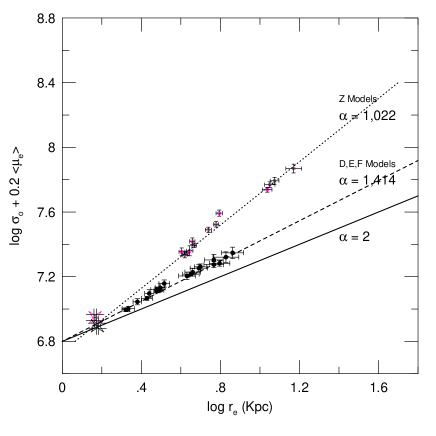
We follow the method given by CdCC95 to compute the characteristic FP variables ($r_{e}$, $\mu_{e}\equiv-2.5\log I_{e}$ and $\sigma_{0}$) of the simulated models. The variables $\sigma_{0}$ and $\mu_{e}$ were combined in the vertical axis according to the usual representation of the FP projected onto the cartesian plane $\log{r_{e}}\times\log{\sigma_{o}}+\beta\mu_{e}$. In all the cases the 3-variate best-fit solutions for a plane gave $\beta=\rm 0.2$ to within 10%, so we decided to keep this coefficient fixed at 0.2 in order to find the orthogonal least squares solutions for the other coefficients, viz. the slope $\alpha$ (the FP ‘tilt’), and the intercept of the fitted plane.

Before analysing the final simulated models in the FP space, however, it is worth to comment that they reproduce the general structural characteristics of elliptical galaxies, e.g. projected triaxialities (from E0 to E5 elliptical objects) and surface density profiles (following the Sersic law). A detailed discussion on the structural properties of the simulated models is given in Dantas (2001).

In Fig. 1 we present the characteristic FP parameters of the objects resulting from the merging of one (D, E e F mergers) and two (Z mergers) component models. In the case of two-component models, the data shown in this figure are relative to the luminous component. The best fit values of the FP slope ($\alpha$) found for these simulations are indicated in the figures. The continuous line ($\alpha=2$) represent the prediction of the virial theorem for homologous, constant $M/L$, systems. In Table 7, we present the results of the best fit values of the data here discussed as well as the results obtained by CdCC95 and DCRdC01. The results indicate that one-component Hernquist mergers (D, E, F) also reproduce reasonably the FP tilt of the elliptical galaxies, consistent with the results obtained with the King models of CdCC95. That is, for both cases, the FP slopes are consistent, within the errors, to that observed for infrared FP of nearby galaxies, that is, $\alpha=1.53\pm 0.08$ (Pahre, Djorgovski & de Carvalho 1998).

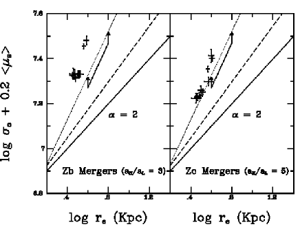
On the other hand, the luminous/barionic objects resulting from the the two-component mergers form a family with a steeper relation in comparison to one-component mergers. (It is interesting to note that if we consider an equivalent to the FP space but for the dark halos of these merger remnants, we find that they constitute an approximate homologous family of objects, as indicates the value $\alpha=1.872$, in Table 7.) In order to test the effects of a more compact halo on these results, we ran two groups of two-component Hernquist mergers with different ratios for the halo to luminous radius (as discussed in Section 2.2.2). Unlike the Z models, these runs were not followed for subsequent (viz., second, etc) generations because of CPU time limitations. In Fig. 2, we show how these more compact halo mergers distribute in the FP space. The arrows over the dotted lines in that figure represent the range occupied by the first generation Z models ($a_{H}/a_{L}=10$), for comparison. It is interesting to notice that the luminous component of the most compact halo models (Zb models), with most negative $E_{orb}$’s, tend to cluster in the FP space in a similar manner as the K collapses. All other models tend to spread out sensibly along a FP-like relation. Also, the luminous body of these models (Zb and ZC models) tend to settle into systematically lower values of $r_{e}$ and at higher values of $y$ ($\equiv\log\sigma_{0}+0.2\langle\mu_{e}\rangle$) than the Z models ($a_{H}/a_{L}=10$). The FP ‘tilts’ of these models suggest a marginally steeper ‘tilt’ than the Z models.

Figure 2: Results for the luminous component of the Hernquist merger simulations, using more compact halos. Left panel: Zb mergers Right panel: Zc mergers. The three lines on these panels are reproductions of the fits shown in Fig.1, for comparison. In particular, the solid line is the prediction of the virial theorem for homologous systems. The arrows over the dotted line represent the range occupied by the first generation Z models ($a_{H}/a_{L}=10$), for comparison.

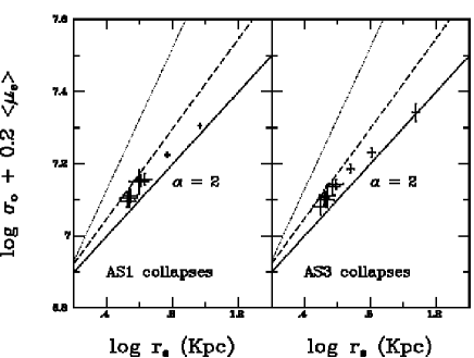
As already mentioned, we have performed two groups (AS1 and AS3 models) of collapse simulations with initial spin in order to verify the effects of the inclusion of rotation on the results by DCdCR01, where evidences for homology were found for pure collapses. The resulting FP ‘tilts’ for both groups ($\alpha_{AS1}=2.204\pm 0.158$; $\alpha_{AS3}=2.306\pm 0.250$) suggests that the resulting models are slightly non-homologous, but in the opposite (viz. $\alpha>2$) sense from the observed FP ‘tilt’ of elliptical galaxies (c.f. Fig. 3).

All these new collapse models evolved for more than $2$ Gyr ($\sim 30T_{cr}$), however, the “hottest” models (viz., AS1-09 and AS3-09, both with initial $\log 2K/|W|=-0.01$) still presented a virial ratio oscillating around $2K/W\sim-1.4$ by that time. These “hottest” models seem to evolve very slowly and still did not reach complete virial equilibrium after $2$ Gyr, whereas all the other models were already well virialized. Removing these “hottest” collapse models results in $\alpha_{AS1-0.01}=1.966\pm 0.270$ and $\alpha_{AS3-0.01}=2.190\pm 0.349$, which are compatible with homology.

Although we cover a reasonable range of $\beta$’s, it is not clear whether the inclusion of more intermediate $\beta$ collapses would necessarily improve the statistics (i.e., decrease the error bar of the fit), since the “coldest” models tend to cluster in the FP space. On the other hand, the inclusion of “hotter” collapses would only exacerbate the observed “inverted” (viz. $\alpha>2$) non-homology. These results seems to indicate that an initial spin is not sufficient to produce non-homology, at least of the same nature of mergers.

Figure 3: Results of the collapse simulations with initial spin in terms of the FP paremeters. Left panel: AS1 collapses, constructed from the progenitor of the “A” models. This progenitor received a solid body rotation resulting on a $\sim 5\%$ perturbation to the initial total kinetic energy of the system, and then “cooled” by a range of $\beta$ factors. Right panel: AS3 models, produced in similar manner as the AS1 collapses, but receiving a larger initial rotational perturbation ($\sim 38\%$). The three lines on these panels are reproductions of the fits shown in Fig.1, for comparison. In particular, the solid line is the prediction of the virial theorem for homologous systems.

Table 7: PF Best Fit Values

Model	$\alpha\pm\delta\alpha$	$N_{fit}$
One-component Models:
D, E, F Mergers	$\alpha=1.414\pm 0.132$	20
King (CdCC95) Mergers	$\alpha=1.36\pm 0.08$	17
K Collapses	no fit: cluster of data points	17
C Collapses:
n = 0	$\alpha=2.070\pm 0.123$	10
n = 1	$\alpha=2.161\pm 0.087$	19
n = 2	$\alpha=2.033\pm 0.342$	10
A Collapses	$\alpha=1.954\pm 0.123$	22
AS1 Collapses (all)	$\alpha=2.306\pm 0.250$	9
AS1 Collapses (removing AS1-09)	$\alpha=2.204\pm 0.158$	8
AS3 Collapses (all)	$\alpha=2.190\pm 0.349$	9
AS3 Collapses (removing AS3-09)	$\alpha=1.966\pm 0.270$	8
Two-component Models:
Z models ($a_{H}=10~{}a_{L}$):
luminous comp.	$\alpha=1.022\pm 0.046$	13
dark comp.	$\alpha=1.872\pm 0.152$	13
both components	$\alpha=1.176\pm 0.070$	13
Zb models ($a_{H}=3~{}a_{L}$):
luminous comp.	$\alpha=1.004\pm 0.123$	9
Zc models ($a_{H}=5~{}a_{L}$):
luminous comp.	$\alpha=1.017\pm 0.105$	9

3.2 Spin Analysis

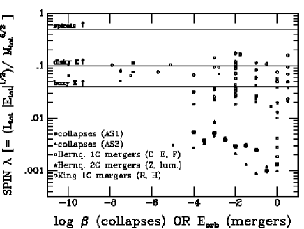
In this section we briefly analyse the how the final spin of the models depend on the initial condition. We parametrize the spin by the dimensioness quantity $\lambda$, defined by (c.f. Peebles 1971):

$$\lambda={L|E|^{1/2}\over GM^{5/2}},$$ (4)

where $L$ is the total angular momentum of the system about its baricenter, $E$ the total energy of the system, and $M$ the total mass (as already mentioned, $G=1$).

Figure 4: Distribution of the spin of the mergers as a function of the initial orbital angular momentum of the pre-merger pair.

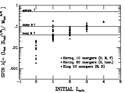
Fig. 4 shows how the spin of the mergers distribute as a function of the initial orbital angular momentum of the pre-merger pair. First, it can be seen that indeed there is a transfer of $L_{orb}$ to the final spin of the merger, since higher $L_{orb}$’s produce systematically higher final spins. Second, intermediate $L_{orb}$’s ($1~{}<~{}L_{orb}~{}<~{}3$) produce objects with spins compatible with boxy ellipticals. We note, however, that the position of the merger products on the FP depends very little on $L_{orb}$ (c.f. CDCC95). In other words, $L_{orb}=3$ mergers could perfectly be produced from $L_{orb}=0$ mergers, and the final products would have approximately the same positions on the FP.

Fig. 5 plot both mergers and collapses as a function of the initial conditions $E_{orb}$ and $\beta$, respectively. It can be seen that mergers from a wide range of $E_{orb}$’s are able to produce objects in the observed range of ellipticals, as opposed to collapses, which fail in this respect. It is interesting to notice that “colder” collapses reach a higher degree of final spin than the “hottest” ones. This seem to imply that the initial rotational pertubations are amplified in the “coldest” collapses. Yet, as we have seen, these “colder” objects still manage to become approximately homologous (see fits for $AS1-09$ and $AS3-09$ sequences in Table 7). Evidently, these results must be interpreted with caution, since we did not reconfigure the initial structure of the progenitor in order to include higher initial spins.

Figure 5: Distribution of the spin of collapses and mergers as a function of the initial collapse factor ($\beta$) and orbital energy ($E_{orb}$), respectively.

3.3 The Virial Coefficients

We use another diagnostics for testing homology on the final simulated objects. A good quantitative measure in this case is the direct computation of the kinematical-structural or virial coefficients ($C_{r},C_{v}$), as described in CdCC95 and DCdCR01:

$$C_{r}\equiv r_{G}/r_{e}$$ (5)

and

$$C_{v}\equiv\langle v^{2}\rangle/\sigma_{0}^{2};$$ (6)

where $r_{e}$ is the effective radius (the radius that defines a sphere containing half of the total luminosity of the system): $L(<r_{e})=L_{tot}/2$. $\sigma_{0}$ is the central projected velocity dispersion, and $r_{G}$ is the gravitational radius, defined by $r_{G}\equiv GM^{2}/|W|$, where $W$ is the total potential energy of the system. $I_{e}\equiv{L(<r_{e})/\pi r_{e}^{2}}$ is the mean surface brightness within $r_{e}$, in linear units. Then, $I_{e}=C_{I}\left({M/2\over\pi r_{e}^{2}}\right)$, with $C_{I}\equiv\left({M\over L}\right)^{-1}$. Inserting the equations above into the virial relation ($\langle v^{2}\rangle={GM/r_{G}}$), we find that $r_{e}=C_{vir}\sigma_{0}^{2}I_{e}^{-1}$, where:

$$C_{vir}\equiv{C_{r}C_{v}\over 2\pi GC_{I}}.$$ (7)

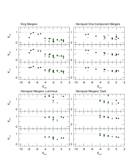
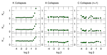
Since, by construction, $C_{I}$ (viz. $M/L$) is constant among the models, the computation of $C_{r}$ and $C_{v}$ directly gives the measure of non-homology among the simulated models. Note that for two-component systems, $r_{G}$ and $\langle v^{2}\rangle$ are calculated from, respectively, the total potential and kinetic energy of the system. Values of $\sigma_{0}$ and $r_{e}$ correspond, however, only to the visible/barionic matter. As already pointed out, non-homologous objects are those which the kinematical-structural coefficients assume different values for each object. The results are presented in Fig. 6, where we plot the coefficients as a function of the initial conditions.

First, we find that the structural coefficients, $C_{r}$, attain different ranges of values for one and two-component models: for one-component mergers, $2.5{~{}}^{<}_{\sim}~{}C_{r}{~{}}^{<}_{\sim}~{}3.5$; whereas for two-component mergers, $8{~{}}^{<}_{\sim}~{}C_{r}{~{}}^{<}_{\sim}~{}15$. This difference is due to the presence of the massive halo in the two-component models, which pushes the gravitational radius to larger values, as compared to the one-component systems. This increase of $r_{G}$ cannot, however, be compensated by $r_{e}$, which depends only on the structure of the luminous core. The kinematical coefficients, $C_{v}$, on the other hand, show similar ranges for both types of mergers. The product $C_{r}C_{v}$ (c.f. upper panel of Fig. 6) therefore attain larger values for two-component models than for one-component ones.

A more relevant aspect of Fig. 6 is the fact that the kinematical/structural coefficients vary in a systematic manner as a function of the initial orbital energy of the merging models, which is in agreement with the results found by CdCC95. This behaviour seem to be an important feature distinguishing mergers from collapses. Indeed, collapses as a whole are approximately homologous objects, although some distinctions between “cold” and “hot” collapses are found (detailed discussion for collapses can be found in DCdCR01). There seems to be no correlation with the orbital angular momentum, as can be seen from an inspection of Fig. 6. On the other hand, it can be seen that the deviation from homology is more accentuated for two-component mergers: If we take the total fractional difference of $y(E_{orb})\equiv(C_{r}C_{v})/2\pi$, $\delta y\equiv|y(E_{orb~{}max})-y(E_{orb~{}min})|/y(E_{orb~{}max})$, we find $\delta y\sim 0.9$ for two-component mergers whereas $\delta y\sim 0.5$ for one-component models ($\delta y$ is $\sim 0$ for homologous objects). This quantity therefore reproduces the deviation from homology as pictured in the FP space (c.f. Fig. 1), with the advantage that it is possible to trace the source of non-homology from the corresponding fractional differences of the $C_{r}$ and the $C_{v}$ coefficients separately. For one-component mergers, $\delta(C_{r})\sim 0.14$, $\delta(C_{v})\sim 0.25$; for two-component mergers, $\delta(C_{r})\sim 0.38$, $\delta(C_{v})\sim 0.42$. Therefore, for one-component mergers, $C_{v}$ contributes more to the non-homology than $C_{r}$, a feature that can be seen clearly from an inspection of Fig. 6.

Figure 6: Ratio of the virial coefficients $C_{vir}$, $C_{r}$ and $C_{v}$ as a function of the initial conditions. Symbols are: 5-point stars for the D models; 3-point stars for the E models; 7-point stars for the E models; 6-point asterisks for the Z models (1st. gen.); 4-point asterisks the for Z models (2nd. gen.); open circles for the King models (1st. gen.); open squares for the King models (2nd. gen.); and open triangles for the King models (3rd. gen.). A dashed horizontal line is indicated and represents an arbitrary homologous family of objects for comparison.

3.4 The Ratio of “Central” to “Envelope” Kinetic Energies

The results of the previous section demonstrate that the (central) non-homology effect which characterizes our merger simulations has a predominant kinematical origin. Now we will analyse the behavior of the total kinetic energy interior to a given radius as compared to the corresponding kinetic energies exterior to that radius. In other words, if we call $K_{tot}(<r)$ the “central” kinetic energy of the the system and $K_{tot}(>r)$ the kinetic energy of its “envelope”, then a measure the ratio of these quantities,$K_{x}\equiv K_{tot}(r>xr_{h})/K_{tot}(r<xr_{h})$, normalized to its progenitor value, should reveal, at least in a gross sense, the effects of the process of relaxation. This process will therefore be viewed as alterations of the kinetic energies of the more gravitationally bounded (“central”) particles against the less bounded ones (“envelope”). Thus if $K_{x}=1$ then the end product model presents the stratification of kinetic energies similar to the progenitor model. If however $K_{x}<1$ then the “central” particles are “hotter” than the “envelope”, as compared to the progenitor.

We analysed the kinetic energy ratio, $K_{x}$, as a function of the initial conditions (collapse factor or orbital energies, for the mergers), for three different radii ($x=0.2$, $0.5$ and $1$). The results are shown in Fig. 7 for the mergers models and in Fig. 8 for the collapse models.

Figure 7: Ratio of the kinectic energies exterior and interior to three distinct radii: $0.2r_{h}$, $0.5r_{h}$, e $1r_{h}$ [notation of the figure: $K_{x}\equiv K_{tot}(r>xr_{h})/K_{tot}(r<xr_{h})$, normalized by the corresponding value of the progenitor (unperturbed model)], as function of the initial conditions. The dashed line indicates that the value of $K_{x}=1$. The symbols are: diamonds for the first generation, circles for the second generation, and crosses for the third generation.

Figure 8: The same as previous figure, but for collapses.

Most collapse models present $K_{x}<1$ for any $x$. The “hottest” K collapses on the other hand approach $K_{x}\rightarrow 1$. In other words, the values of $K_{x}$ do not change with the initial collapse factor ($\beta$), except for the “hottest” K collapses. Moreover the values of $K_{x}$ are similar among different models, except, possibly, the C models which seems more noisy than the others. For larger $x$, all the collapse models have $K_{x}\rightarrow 1$. The general trend is that the collapse models are centrally “hotter” than the corresponding progenitor, independently of the initial $\beta$ (except for $\beta$’s very close to $1$) and the initial model used.

The stratification of kinetic energies in the case of mergers is not similar to the collapses. For mergers, it is clear that $K_{x}$ is a systematic function of the initial orbital energy of the pairs. In other words, for mergers with more negative initial orbital energies $K_{x}\rightarrow 1$, showing no difference with their progenitors, whereas the ones with less negative energies deviate more from the progenitor, and in a systematic way, towards $K_{x}<1$. The magnitude of the deviation from $K_{x}=1$ also depends on the merging models: for instance, is greater for the King models, intermediate for the Hernquist one-component models, and smaller for the Hernquist two-component models. It also seems to slightly increase for increasingly merger generations. There are also examples where $K_{x}>1$ (some Hernquist two-component models, with $x=0.2$). In other words, the behavior of $K_{x}$ for mergers seems to be more complex than collapses and shows a clear systematic dependency on the initial orbital energy of the pairs, in the same sense that the virial coefficients depend systematically on $E_{orb}$.

In case of mergers, the systematic dependency of $K_{x}$ on $E_{orb}$ begins to flatten and tend to be erased for sufficiently large values of $x$. This in fact shows that the merger models tend to a similar stratification of the “central” and “envelope” kinetic energies at sufficiently large radius. In other words, the different $K_{x}$ values among the merger models are not only a function of the initial orbital energy but is a function of $x$ as well, so that the correlation $K_{x}\times E_{orb}$ is stronger at the very center of the models and tend to disappear at sufficiently large radii. This shows therefore that the effect is intimately related to the central parts of the system.

Our detailed description of the ratio of kinetic energies behaviour among models, as given in this section, seem to reinforce the idea that the non-homolgy in mergers is a central effect ruled by how the particles gain kinetic energy during the merger. In other words, the non-homology seem to have a dynamical origin which is not present in simple collapses.

In the following, we focus on the analysis of the relaxation history of both mergers and colapses, which may help us to find clues for understanding the dynamical processes that are at the origin of the non-homology of mergers.

3.5 Relaxation Histories

3.5.1 Evolution of the Virial Ratio $2K/W$

In order to trace a measure of the fluctuations of the gravitational potential on its way to equilibrium, we compared the behaviour of the virial ratio $2K/W$ (measured for the whole system, including escapers) during the evolution of different and representative types of models, namely: a “cold” (A01 model, $\log\beta=-4$) and a “hot” (A09 model, $\log\beta=-0.75$) collapse; against a “rapid” (D10 model, $E_{orb}=-5$, $L_{orb}=0$) and a ”slow” (D9 model, $E_{orb}=0$, $L_{orb}=3$) one-component merger. Fig. 9 shows the behaviour of these representative models. Notice that some models do not stabilize around $2K/W=-1$, as would be expected for a virialized model. This is due to the fact that we are measuring the virial coefficient using the complete particle data, including particles with positive energies which have escaped the system. More “violent” relaxations produce more escapers, and the resulting virial ratio stabilizes around some other value slightly different than $-1$.

Figure 9: The behaviour of the virial ratio $2K/W$ during the evolution of different and representative types of models. Upper panel: collapses. Lower panel: mergers.

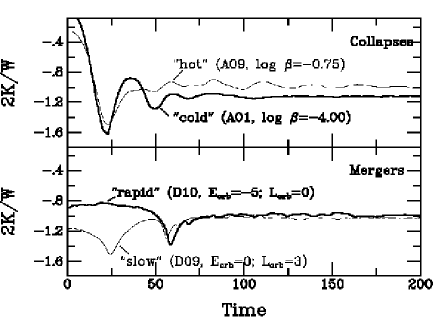
We notice that the most rapidly merging system suffer only one major fluctuation of $2K/W$, subsequently rapidly reaching equilibrium. The slower merger shows that $2K/W$ varies in large periods during the first moments of the evolution (in other words: it does not show a unique abrupt change in $2K/W$, but rather two or more large periodic fluctuations before reaching equilibrium). Collapses, regardless of being “cold” or “hot” show one large initial fluctuation amplitude in $2K/W$. Interestingly, subsequent evolution seem to be different: the “cold” collapse still experiences one more relatively significant fluctuation of $2K/W$ before reaching equilibrium. The “hot” collapse, on the other hand, show a persistent, although of low amplitude, fluctuation of $2K/W$ still for some time, when the “colder” collapse is comparatively well stabilized.

3.5.2 The ‘Kandrup’ Effect

In order to understand the dynamical behaviour presented by the simulated models, we apply a diagnostic advocated by Kandrup et al. (1993). The merging of stellar systems occurs because of a transfer of the orbital energy to the particles of the stellar systems in question. The mechanisms through which this occurs are the tidal interactions, which increase the internal energy of the systems at the expense of their orbital energy. The question here concerns the relation of this mechanism with the central non-homology of the simulated mergers.

During the evolution of the system, the energy of the particles is not, in general, conserved, even in a “coarse grained” sense (viz. through the distribution $N(E)$; for a discussion on the importance of this distribution for stellar systems, see Binney 1982). Kandrup et al. studied the distribution of the energy of the particles in systems resulting from collisions (without the formation of a final single object) and merging of two galaxies. These authors found that there is a “coarse-grained” sense in which the ordering of the mean energy of given collections of particles is unaltered, even though $N(E)$ may vary substantially. In this section, we revisit the question raised by Kandrup et al. and try to connect this fact to the behaviour of the simulated systems in context of the FP. Notice that their conclusions were based on only two simulations of collisions, with only one merger, and two collapses. Here we use a much larger set of simulations and initial conditions, and a larger number of particles as compared to the models used by Kandrup et al. We will not consider time evolutions of mean energies, as Kandrup et al. did, but only the initial and final values of the mean energy of the given collections of particles. We discuss further their diagnostic below.

The method may be considered a “lagrangian” approach to the analysis of how the energy of the particles change because of the relaxation process. The particles of the initial models have been sorted accordingly to their binding energies and the models were partitioned into 5 bins of equal number of particles (a finer partitioning with 10 bins produced essentially the same results). For each of these bins, the mean energy was calculated and the bins ranked with the first one initially containing the most bound particles (most negative mean energy) whereas the fifth, the less bounded ones (less negative mean energy). The mean energy of these collections of particles were then recalculated at the end of the run’s and compared with their initial values. We have limited our analysis for the first generation of mergers. In the case of mergers with equal $E_{orb}$’s, we have included only the model with lower $L_{orb}$. The results of these comparison are displayed in Figs. 10 and 11.

Figure 10: Energy means of $5$ equal number collections of particles, ordered accordingly to their initial mean binding energies. The initial and final mean binding energy values are connected by a line segment (left extreme: initial mean value; right extreme: final value), centered in the initial condition of each model. “Bin numbers” are indicated in the figure: bin number $1$ refers to the most bounded particles; and successively throughout bin number $5$, which refers to the most weakly bound particles. The values of the final mean binding energy of the initially most bounded bin (1) are connected with a dashed line, illustrating how it changes as a function of the initial condition. The models shown are collapses.

Figure 11: The same as previous figure, but for first generation mergers. In the case of mergers with equal $E_{orb}$’s, we have included in the figure only the model with lower $L_{orb}$.

We found that, except for some of the C cases, collapses preserve the ordering of the mean energies per bin entirely. These results confirm the findings of Kandrup et al. Moreover the mean energies per bin that changed more in this case were the ones corresponding to the most bounded bins (1, 2, 3, etc). The central potential becomes deeper after the collapse, and the particles initially more bounded to the system tend to loose energy, becoming even more tied. This effect is also a function of the collapse factor $\beta$, as can be seen by the dashed line in the figure, which connects the most bounded bin (1), illustrating how this bin changes as a function initial condition. In the case of A collapses, the mean energies representing the three less bounded bins converge to similar final values, whereas the two most strongly bounded bins reach even more negative mean values. This behaviour indicate that collapses tend to produce core-halo structures. In the case of C collapses, the mean energies change considerably and chaotically. Recall that these models contain a Hubble flux which may favor the grow of perturbations embedded in these models, adding some complexity in the evolution of the mean energy of these distinct collections of particles.

In the case of mergers (one and two-component models), the preservation of the ordering of the mean energies per bin is not as good as in the case of collapses. For the D models (Hernquist one-component models), the initially most bounded particles will remain as the most bounded ones after the relaxation process. However, it can be seen that the bins number 3 actually cross bins number 2 and reach the values corresponding to bins number 1. In the case of two-component models, the luminous matter tend to reach very negative values of the mean energies, almost converging to similar values for all bins. The general behaviour of the luminous component resemble the behaviour of the most boundly tied particles of the collapse models. The main reason for this may be the fact that, after the initial interaction, the luminous component finds its equilibrium state within the deeper potential well of the dark halo. This might occur through a partial collapse of the luminous matter inside the dark halo. In the case of the dark matter component, there is also some violation of the ordering of the mean energies per bin. In fact, the initially most boundly tied bins (number 1) crosses upwards and gain energy in some cases. The halo seems to be the only system that actually shows clearly this behaviour.

The D models and the luminous component also present the same effect as seen in collapses: the particles initially more bounded to the system tend to loose energy as a function of the initial orbital energy, as can be seen by the dashed line in the figure, which connects the most bounded bins (1). For halos, this behaviour is not as clear.

Note that the mean biding energy of the most bounded bins remains at an almost constant value for collapses (see dashed lines in Fig. 10), rising steeply for the “hottest” collapses. The C models present more fluctuations in this behaviour. For mergers, on the other hand, these changes proceed more smoothly and systematically with the initial orbital energy (dashed lines in Fig. 11). This means that the initially most bounded collection of particles remain at the average the most bounded particles after the relaxation, but at a more negative mean energy than the slower (less negative $E_{orb}$) mergers.

It is clear that if the ordering of the mean energies of particles, partitioned at a coarse-grained level, is strictly conserved, as in collapses, then the most bounded particles (in average closer to the baricenter) continue be the most bounded particles after virialization. However, as pointed out previously, this ordering conservation does not occur for mergers. In other words, some complex behaviour seem to take place during the merger involving the more central or bounded particles, an effect which does not occur at all in collapses (except for some small shuffling between the less bounded bins for the “hottest” C models). In summary, we entirely confirm the results of Kandrup et al. for collapses, but in the case of mergers, some violation of the ordering conservation of the energy bins is present.

4 Discussion

We have simulated a hierarchical non-dissipative merger scheme similar to that of CdCC95, however using different models for representing the progenitors of the $\rm 1^{st}$ generation mergers. In contrast with CdCC95, which considered King density profiles, we used models endowed with cuspy profiles, such as the Hernquist density profile. Also models with a dark halo second component were used in this study. A comparison with collapse simulations (previously analysed in DCdCR01 and here extended to include collapses with initial spins) is presented.

We found that the one-component Hernquist mergers give results similar to those found by CdCC95 for the one-component King models, namely both were able to build-up small scattering FP-like correlations with slopes consistent to those found for the near infrared FP of nearby galaxies. The two-component models also reproduce a FP-like correlation, but with a significantly steeper slope which is in agreement with that found for galaxies at high redshift (Pahre 1998). Pahre finds that the slope of the near-infrared FP decreases with increasing redshift (see his Figure 7.2). Another important piece of evidence of the evolution of the FP with redshift comes from the work of Kelson et al. (1997). The authors find that the structure of the galaxies in the analysed sample has not changed significantly since $z=0.58$, based on the fact that the observed scatter is rather low: $\pm 0.067$ in $\log r_{e}$. Besides, they find a dependence between $M/L_{V}$ and redshift, which reinforces the idea of a stellar population effect in the evolution of the FP.

In nature, dissipational effects must have played a role in producing the FP relations and their scatter, but it would be unwise to completely disregard the role of stellar dynamics in shaping ellipticals as well. Our simulations are only of a dynamical character, with the $M/L$ ratio fixed by construction. Systematic non-homology in the evolved models can produce FP-like ‘tilts’ compatible with those found in nature. In particular, we show the importance of the gravitational potential of the halo for changing the ‘tilt’ of the FP: the magnitude of the change can be seen directly from a comparison between one-component and two-component Hernquist merger models (c.f. Fig. 1). In other words, this simple result clearly shows how the FP slope may be dynamically changed just by the addition of a halo. Therefore, our results suggest that the structure evolution of the halo could also have a collateral importance in changing and shaping the FP ‘tilt’, along with population evolution effects (e.g. Kelson et al. 1997). We speculate on the possibility that halos may suffer evolution from $z\sim 0.5$ to the present. The evolution could be in the form of tidal stripping, which would decrease the mass of the halo, or by the presence of supermassive central black holes, which could alter the matter distribution of the halo, forming a core (c.f. Hennawi & Ostriker 2002). If dark matter presents some level of self-interaction (c.f. Spergel & Steinhardt 2000), then it may drive evolution towards a core in less than a Hubble time (c.f. Yoshida et al. 2000). If some of these processes have operated in halos during the past few Gyrs, in the sense of altering their gravitational potentials at the centers of galaxies, the characteristic scaling properties of the luminous/barionic component might have changed as well. Whether any of these possibilities are in factible is at present an open issue.

A qualitative analysis of the behaviour of the mean energy of collections of particles (as advocated by Kandrup et al. 1993) lead us to consider the possibility that ‘mesoscopic’ constraints could have some connection to the central non-homology. The conservation of the ordering of the mean energy of collections of particles implies that the process of ‘mixing’ in the one-particle energy space is quite inefficient as compared with ‘mixing’ in configuration and/or velocity space (see discussion in Kandrup et al.). This seem to be true for collapses, but not entirely for the central parts of mergers.

The most intense tidal perturbations (shocks) seem to be found for the most rapidly merging systems (more negative orbital energies). In this case, the particles probably withdraw the energy from the relative orbit of the merging pairs at one major fluctuation. Secondary fluctuations on the gravitational potential evolve afterwards rapidly and reach equilibrium in a short timescale as well. The stratification of the kinetic energies resemble that of the progenitor in this case. On the other hand, if the orbital energy is less negative (slow mergers), there is some of time for the particles to withdraw energy from the orbit of the pair, and this process involves periodically large fluctuations on the potential that evolve slowly, taking a larger amount of time to stabilize. This process may be important in “heating up” the central parts of the models approaching $E_{orb}\rightarrow 0$. This should be important in defining the non-homology in mergers because the stratification of the kinetic energies are indeed different to that of the progenitor.

On the other hand, in the case of collapses, the dynamics seem to operate in a different manner than in mergers. Collapses starts off from a spherically symmetric condition that mergers do not share. Collapses also produce not only fast by very high amplitude gravitational potential fluctuations that dump rapidly. This process should be very efficient in heating up the central parts of the models in configuration and/or velocity space, but not efficient enough to have the particles ‘forget’ their initial energies in a collective (‘mesoscopic’) manner. As already pointed out by Kandrup et al., this behaviour is at odds with Lynden-Bell’s theory of ‘violent relaxation’, where ‘mixing’ in energy space is not expected to be inefficient for any given collection of particles. At the same time, we have found that collapses seem to ‘prefer’ forming homologous systems, whereas mergers do not. Some connection between ‘mesoscopic’ constraints and non-homology seem to be apparent, but this is an open question.

We did not atempt at this time to rigorously try to connect the behaviour of the violation of the ordering of the energy bins (Figs. 11 and 10) with the behaviour of the ‘central’ to ‘envelope’ kinetic energies (Figs. 7 and 8). Although interesting, in order to fully understand this effect, we would need to probe the problem of relaxation in a much deeper and/or formal manner, which is not the objetive of our paper at the present time. Figs. 11 and 10 illustrate a diagnostic on the behaviour of the change of energy of the system due to relaxation in a ‘mesoscopic’ scale. Figs. 7 and 8 show a different dignostic, where the change of energy of the central and external parts of the system are compared to their progentor models, not the to their initial condition (as in Figs. 11 and 10), and hence refer to a more ‘macroscopic’ feature of the relaxation process. On the other hand, the main point of Figs. 11 and 10 is not to show how the energy of collections of particles change due to relaxation (although it also certainly shows that) but in what degree the ordering of their mean energies is violated. This type of analysis was first envisaged by Kandrup in 1993 and is still not well understood. In our oppinion, it is not at all clear how one could find any immediate connection between both sets of figures. We know that the non-homology comes primarily as a systematic function of $E_{orb}$. Both sets of figures show systematic behaviour of 2 different types of diagnostics as a function of $E_{orb}$. Collapses show almost no dependecy of these same diagnostics with $\beta$ (except for the “hottest” collapses). Therefore, it seems that relaxation through merging embodies some mechanism which is effective in differentiating the final models, producing non-homology, whereas this mechanism is absent or highly precluded in collapses (again, except for the “hottest” ones, which are just a small perturbation form equilibrium of the progenitor model). In fact, what is lacking in order to make any progress in this direction is a systematic understanding of the nature of the gravitational relaxation mechanism, where several conceptual issues are still unsolved (c.f. Padmanabhan 1990).

In any case, our results seems to strenghten the idea that dissipationless merging could produce significant non-homology in the final objects and therefore FP-like relations in the same sense and with comparable values of the FP ‘tilt’ as those observed in ellipticals. We have shown that, from purely dynamical grounds, mergers can produce FP-like relations while simple collapses cannot (two-component collapses were not investigated here and will be a subject for future work). The evolution of gradients in the gravitational field of the merging galaxies seem to dictate the final non-homology of the end products. Further investigations are necessary in order to stablish, quantify and rigorously explain these complex effects, as preliminary discussed in this paper.

References

- Aguilar & Merritt (1990) Aguilar, L. A. & Merritt, D., 1990, ApJ 354, 33.
- Barnes & Hut (1986) Barnes,J. & Hut, P., 1986, Nature v.324, 446.
- Bekki (1998) Bekki, K., 1998, ApJ, 496, 713.
- Bender & Saglia (1999) Bender & Saglia, 1999, astro-ph/9811416. In Galaxy Dynamics, ASP Conf. Series Vol. 182 (San Francisco: ASP), edited by David R. Merritt, Monica Valluri, and J. A. Sellwood, page 113.
- Binney (1982) Binney, J., 1982, MNRAS 200, 951.
- Binney & Tremaine (1987) Binney, J. & Tremaine, S., 1987, Galactic Dynamics (Princeton: Princeton Univ. Press).
- Burkert (1995) Burkert, A., 1995, ApJ, 447, L25.
- Burstein et al. (1997) Burstein, D., Bender, R., Faber, S. M., & Nolthenius, R., 1997, AJ 114, 1365.
- Busarello et al. (1997) Busarello, G., Capaccioli, M., Capozziello, S., Longo, G., & Puddu, E., 1997, A&A, 320, 415.
- Capelato, de Carvalho & Carlberg (1995) Capelato, H. V., de Carvalho, R. R. & Carlberg, R. G., 1995, ApJ, 451, 525.
- Capelato, de Carvalho & Carlberg (1997) Capelato, H. V., de Carvalho, R. R. & Carlberg, R. G., 1997, in Galaxy Scaling Relations: Origins, Evolution and Applications, proceedings from the ESO Workshop held November, 1996, edited by Luiz Nicolaci da Costa and Alvio Renzini (Springer-Verlag), p. 331.
- Carpintero & Muzzio (1995) Carpintero, D. D. & Muzzio, J. C., 1995, ApJ, 440, 5.
- Ciotti, Lanzoni & Renzini (1996) Ciotti,L., Lanzoni,B., Renzini, A., MNRAS, 282, 1.
- Cole et al. (2000) Cole et al., 2000, MNRAS 319, 168.
- Dantas et al. (2000) Dantas, C. C., Ribeiro, A. L. B., Capelato, H. V., & de Carvalho, R. R., 2000, ApJ, 528, L5.
- Dantas et al. (2001) Dantas, C. C., Capelato, H. V., de Carvalho, R. R., & Ribeiro, A. L. B., 2002, A&A, 384, 772.
- Dantas (2001) Dantas, C. C. , 2001, PhD Thesis, Instituto Nacional de Pesquisas Espaciais, Brazil.
- Davé et al. (2001) Davé, R., Spergel, D.N., Steinhardt, P.J. & Wandelt, B.D., 2001, ApJ, 547, 574.
- de Zeeuw & Franx, M. (1991) de Zeeuw, T. & Franx, M., 1991, ARAA, 29, 239.
- Djorgovski & Davis (1987) Djorgovski, S. G. & Davis, M., ApJ, 1987, 313, 59.
- Djorgovski (1988) Djorgovski, S. G., in Proc. Moriond Astrophysics Workshop, 1988, Starbursts and Galaxy Evolution, ed. T. X. Thuan et al. (Gif sur Yvette: Editions Frontières), 549.
- Djogorvski & Santiago (1993) Djogorvski, S. G. & Santiago, B. X., 1993, in Structure, Dynamics and Chemical Evolution of Elliptical Galaxies, Proc. ESO/EIPC Workshop, ed. I. J. Danziger, W. W. Zeilinger, & K. Kjar (ESO Conf. and Workshop Proc. 45) (Garching:ESO), 59
- Dressler et al. (1987) Dressler, A., Lynden-Bell, D., Burstein, D., Davies, R. L., Faber, S. M., Terlevich, R. J., & Wegner, G., 1987, ApJ, 313, 42.
- Dubinski (1988) Dubinski, J. 1988, MS thesis, Univ. of Toronto.
- Gerhardt et al. (2000) Gerhardt et al. 2000, ApJ, 539, L13.
- Gerhardt et al. (2001) Gerhardt et al. 2001, AJ 121, 1936.
- Gott (1973) Gott III, J. R., 1973, ApJ 186, 481.
- Graham & Colless (1997) Graham, A. & Colless, M., 1997, MNRAS 287, 221.
- Hennawi & Ostriker (2002) Hennawi, J. F. & Ostriker, J. P., 2002, ApJ 572, 41.
- Hernquist (1990) Hernquist, L., 1990, ApJ 356, 359.
- Hernquist (1993) Hernquist, L., 1993, ApJ 409, 548.
- Hjorth & Madsen (1991) Hjorth, J. & Madsen, J., 1991, MNRAS, 253, 703.
- Hjorth & Madsen (1995) Hjorth, J. & Madsen, J., 1995, ApJ, 445, 55.
- Kandrup et al. (1993) Kandrup, H. E., Mahon, M. E., & Smith, H., 1993, A&A 271, 440.
- Kelson et al. (1997) Kelson, D. D., van Dokkum, P. G., Franx, M., Illingworth, G. D., & Fabricant, D, 1997, ApJ, 478, L13.
- Kronawitter et al. (2000) Kronawitter, A., A&AS, 144 53.
- Luwel & Servene (1983) Luwel, M. & Servene, G., 1983, MNRAS, 203, 15P.
- Mihos et al. (1998) Mihos et al., 1998, ApJ 494, 183.
- Navarro, Frenk & White (1997) Navarro, J. R., Frnk, C. S. & White, S. D. M., 1997, ApJ, 490, 493.
- Padmanabhan (1990) Padmanabhan, T., 1990, Physics Reports, 188, No.5, 285-362.
- Pahre (1998) Pahre, M., 1998, PhD Thesis, California Institute of Technology.
- Pahre, Djorgovski & de Carvalho (1995) Pahre, M. A., Djorgovski, S. G. & de Carvalho, R. R., 1995, ApJL, 453, L17.
- Pahre & Djorgovski (1997) Pahre, M. A. & Djorgovski, 1997, in The Nature of Elliptical Galaxies, Proceedings of the Second Stromlo Symposium, eds. M. Arnaboldi, G. S. Da Costa, & P. Saha, ASP Conf. Ser. Vol. 116, (San Francisco: ASP), 154.
- Pahre, Djorgovski & de Carvalho (1998) Pahre, M. A., Djorgovski, S. G. & de Carvalho, R. R., 1998, AJ, 116, 1591.
- Peebles (1971) Peebles, P. J. E., 1971, A&A 11, 377.
- Renzini et al. (1993) Renzini, A., Ciotti, L., D’Ercole, A. & Pellegrini, S., 1993, ApJ, 419, 52.
- Salucci & Burkert (2000) Salucci, P., & Burkert, A., 2000, ApJ, 537, L9.
- Siopis et al. (2000) Siopis et al. 2000, astro-ph 0010326. Proceedings of the International Conference on Stellar Dynamics: Classical to Modern, 21-27 August 2000, St. Petersburg State University, edited by L.P. Ossipkov and I. I. Nikiforov, St. Petersburg University Press, page 420-426.
- Spergel & Steinhardt (2000) Spergel, D. N., & Steinhardt, P. J., 2000, Phys. Rev. Lett., 84, 3760.
- Villumsen (1984) Villumsen, 1984, ApJ, 284, 75.
- Walker et al. (1996) Walker, I. R., Mihos, J. C. & Hernquist, L., 1996, ApJ, 460, 121.
- White (1978) White, S.D.M., 1978, MNRAS, 184, 185.
- Wilkinson & James (1982) Wilkinson, A. & James, R. A., 1982, MNRAS 199, 171.
- Yoshida et al. (2000) Yoshida, N., Springel, V., White, S. D. M., & Tormen, G., 2000, ApJ, 544, L87.