$H$-band observations of the Chandra Deep Field South

We report preliminary results of our $H$-band survey of the Chandra Deep Field South (CDFS). The observations were made using SofI on the NTT, and cover 0.027 square degrees with a 50 % completeness limit of $H$ =20.5, and 0.17 square degrees with a 50 % completeness limit of $H$ =19.8. We used SExtractor to extract sources from our fields. In total we have detected 4819 objects. Star-galaxy separation was performed using the SExtractor parameter “stellarity index”. All objects with an index of 0.5 or lower were classified as galaxies. According to this criterion, 80 % of our detections are galaxies. We then compare our results with previous observations of the CDFS. Our astrometric solutions are in good agreement with the Las Campanas Infrared Survey (LCIRS), the COMBO-17 and the ESO-EIS surveys. The photometry of our catalog compares satisfactorily with the results of the LCIRS, as well as with the GOODS data. Galaxy number counts are presented and compared with the LCIRS results. The present data are intended to complement the recent and future multi-wavelenghth observations of the CDFS and will be used, in conjuction with additional multiband photometry, to find counterparts of the upcoming mid-infrared surveys with SIRTF.

1 Introduction

One of the many reasons for performing a deep survey is to study large-scale structure at high redshifts ($z\geq 1$) and to directly probe galaxy evolution from early epochs to present days. Such studies allow us to trace the history of galaxy formation and evolution (Ellis, 2001; Cohen et al., 2000) and to improve our understanding of the sources of the various components of the cosmic background (Totani et al., 2001; Madau & Pozzetti, 2000). High redshift galaxies are often quite faint, and the use of spectroscopy to measure redshifts and other properties can be prohibitively expensive. The alternative way to estimate redshifts for large samples is to apply photometric techniques (Koo, 1985; Fontana et al., 2000; Fernández-Soto et al., 1999; Le Borgne & Rocca-Volmerange, 2002). This approach relies on the detection of typical SED features. Optical (UBVRI) data are able to detect the Balmer Break at 4000 Å  up to $z$ $\sim$ 1.3, and the Lyman Break at 900 Å  for $z$ $\geq$ 3 (Steidel et al., 1995). For 1.3 $\leq$ $z$ $\leq$ 3, the Balmer Break is redshifted beyond the $I$ band and near infrared (NIR) data in the J and H bands are necessary to constraint the redshift with a high enough accuracy.

Currently, one of the best studied fields in the sky is the Chandra Deep Field South (CDF-S), located at J2000 coordinates $03^{\rm h}32^{\rm m}28^{\rm s}$, $-27^{\circ}48\arcmin 30\arcsec$ (Giacconi et al., 2001). The CDF-S is a “blank” region of the southern sky chosen as the target for an extremely deep exposure with the Chandra X-ray Observatory. It has been the subject of observations with other space-based telescopes as well, including the Hubble Space Telescope (Schreier et al., 2001), as well as with numerous ground-based telescopes in the optical (Arnouts et al., 2001; Wolf et al., 2001), near-infrared (Saracco et al., 2001; Chen et al., 2002), and radio (Kellermann et al., 2000). Several sets of mid- and far-infrared observations with the upcoming Space Infrared Telescope Facility (SIRTF; Fanson et al., 1998) are planned, including Guaranteed Time Observations by the IRAC and MIPS instrument teams and Legacy program observations by the GOODS (Dickinson et al., 2002) and SWIRE (Franceschini et al., 2002) projects.

The ESO Imaging Survey (EIS) has performed the most extensive optical-NIR coverage of the CDF-S to date. It includes $UBVRI$ observations covering 0.25 square degrees (Arnouts et al., 2001) and $JK_{s}$ observations covering $\sim$400 square arcminutes (Vandame et al., 2001). Filling the gap between these two filters is required by photometric redshift determination techniques, and implies observations of the CDFS in the H band. The COMBO-17 survey (Wolf et al., 2001) has imaged a $31.5\arcmin\times$30′ field covering the CDF-S in 5 broad-band and 12 narrow-band filters, but with a wavelength coverage limited to the interval between the 3650 and 9140 Å. The Las Campanas Infrared Survey (Firth et al., 2002; Chen et al., 2002) has recently performed $H$-band observations covering $25\arcmin\times$25′ in the CDF-S, down to a 5 $\sigma$ limiting magnitude of $\sim$ 20.5. ; however, their field is not centered on the Chandra observations. We note that the GOODS SIRTF Legacy team is observing a smaller ($10\arcmin\times 15\arcmin$) area of the CDF-S to a much greater depth than our observations, using ISAAC on the VLT. Their first data are available on the ESO web site.

We have conducted an $H$-band survey of the CDF-S, centered on the X-ray field, and encompassing the spatial coverage of the EIS observations as well as the future IRAC pointings. In the present paper we present the results of this survey. The observations and data reduction are described in Section 2; Section 3 presents the source extraction method and the resulting source lists. The survey performance is discussed in Section 4. Our conclusions are summarized in Section 5.

2 Observations and Data Reduction

2.1 Observations

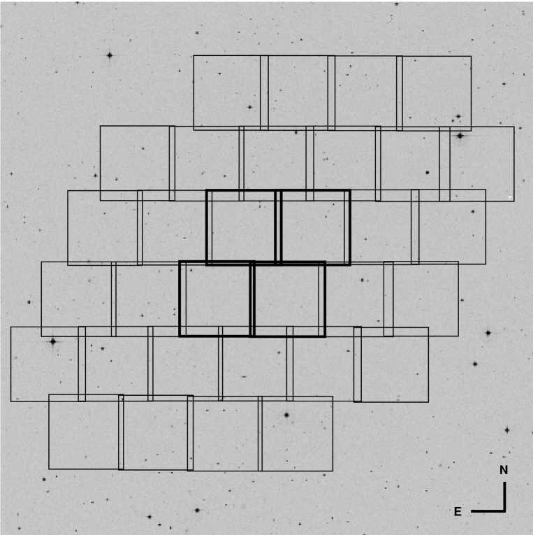
Figure 1: The 32 SofI fields overlaid on a 35′square Digitized Sky Survey image of the Chandra Deep Field South. Each SofI field is 4.9′ square; the deeper central fields are indicated by thicker outlines.

We carried out the observations using the SofI near infrared imaging camera (Moorwood, Cuby & Lidman, 1998) installed on the ESO–NTT telescope at La Silla, during two observing runs: 15–18 November 2000 and 27–30 November 2001. The $H$-band filter of the SofI imaging mode is centered at 1.653 $\mu$m and is 0.297 $\mu$m wide. The SofI detector is a Hawaii HgCdTe 1024x1024 array. Sky conditions were photometric throughout the acquisition of the images with the seeing varying between 0.4–0.8″. We defined 32 $4.9\arcmin\times 4.9\arcmin$ fields covering the CDF-S area (see Figure 1) and observed each of them in the “large field” configuration, with a scale of 0.288″ pixel^-1.

The observations were carried out using the “jitter” technique, one of the most efficient methods of sky acquisition with a minimum loss of observing time. The telescope is offset by small amounts around a central position. Offsets are generated randomly but are restricted within a square box. In our case the box width was 35″. A typical acquisition in jitter mode consisted of 60 1 minute long frames, reaching a total integration time of 1 hr. For the four central fields we repeated the sequence an additional three times, for a total of 4 hours of integration time. Infrared standard stars from the Persson et al. (1998) list were observed every hour at similar airmasses to the science exposures.

2.2 Sky subtraction

Data reduction included the usual steps of flat-fielding (based on dome-flats) and bad pixel fixing, followed by a two-pass sky-subtraction. This method prevents bright objects from affecting the residual sky levels and thus the photometry of faint objects. The jitter routine in eclipse (Devillard, 1999, 1997) was used to make the first-pass sky-subtraction and image registration. jitter does not have an object-masking capability, so we used the dimsum package in IRAF to co-add the first-pass images, derive an object mask from the co-added image, and redo the sky subtraction with objects masked. We then combined the final sky-subtracted images using jitter (which is much faster than IRAF-based tools).

2.3 Astrometry

We performed astrometric calibrations of the images using stars taken from the United States Naval Observatory (Monet, 1998) and 2 Micron All Sky Survey (2MASS) databases. The astrometric solutions were computed using the tasks ccmap and ccsetwcs in the IRAF imcoords package.

In order to check the accuracy of the astrometry our catalogs were compared with the source lists extracted from previous observations of the CDF-S. The relative offsets between the most likely counterparts of our $H$-band detections in the other source lists were computed, and the result is shown in Fig. 2. There is a negligible offset in right ascension and an offset of 0.15″ in declination between our data and the Las Campanas Infrared Survey (LCIRS) catalog. The rms in the difference is $\leq 0.24$″ in both directions. The comparison is particularly good with the result of the COMBO-17 survey. The offsets are quite small ($\leq 0.02$″) in both directions, and the rms is only $\sim 0.2$″. Arnouts et al. (2001) found an offset of $\sim 0.2$″  in $\alpha$ and $\delta$ between the EIS and COMBO images. Not surprisingly, since COMBO astrometric calibrations are very similar to ours, we find a similar shift between our data and the EIS catalogs, $\sim 0.35$″, with a rms of 0.2″.

2.4 Photometric Calibration

We measured the instrumental magnitude of the standard stars in a 10-pixel (2.9″) radius aperture. The magnitude zeropoint of the corresponding exposure was computed as the difference between the instrumental and the cataloged $H$-band magnitudes. The zeropoints are compatible with other results listed on the NTT/SofI web page. Typical changes in the zeropoint over a night are $\leq 0.04$ mag; since this includes real changes with the airmass, this value is probably an upper bound on the zeropoint error. For each CDF-S field (except the four central ones, see below), we took the average of the two values derived from the bracketing standard star observations as the zeropoint. For the co-added images of the four central fields, the median of the zeropoints computed for the individual exposures was adopted.

We tested our photometric calibrations by comparing the magnitudes measured in a similar aperture by the LCIRS team and in the present work. The result is shown in Fig. 3. Our magnitudes are 0.13 mag brighter than those in LCIRS, with an rms of 0.27 for $14\leq H\leq 19$. The cause of this difference is not known. We also checked our measurements by doing photometry on CDF-S H-band images made available by the GOODS team, although the zeropoint for these data is uncertain. We find our aperture magnitudes to be 0.06 mag fainter than those measured on the GOODS images, again with an rms of 0.27 (Fig. 4).

3 Source list

Object detection was performed using version 2.2.2 of the SExtractor package (Bertin & Arnouts, 1996). We performed one SExtractor per field. Each individual catalog was cleaned from spurious detections in the outermost parts of the image, which do not have a full 60-minute exposure time. Thanks to a partial overlap (30 ″) between our pointings, these regions are covered to full depth in adjacent fields, except on the outside of the survey region.

For the extraction we used a 7$\times$7 Gaussian filter with a FWHM of 3 pixels. Weight maps were computed from the image background to improve the quality of the source extraction by taking into account the image quality at each pixel. The SExtractor detection threshold was fixed to a conservative value of 3, and the minimum number of connected pixels above detection threshold to 5 for all fields. The initial catalogs were then cleaned of objects near saturated$/$hot pixels and objects where a reliable estimate of the flux was not feasible.

The final catalog contains 4819 objects, including 956 detections in the four deeper central fields. As an example, the first 40 entries of the final catalog are presented in Table 1. The following quantities are listed:

• Column 1: identification number.

• Column 2 and 3: right ascension and declination (J2000).

• Column 4-7: automatic and isophotal magnitudes and respective errors, as estimated by SExtractor.

• Column 8-9: aperture magnitude (10 pixels, or 2.9″ diameter) and error.

• Column 10: SExtractor stellarity index.

4 Survey performance

4.1 Star-galaxy separation

Star/galaxy separation in deep observations is always challenging. Commonly used techniques are based on object morphology and/or colour properties (e.g. Gardner et al. 19XX, Huang et al., 1997) when available. The SExtractor “stellarity index” (CLASS_STAR) is computed for a given object from the comparison of its luminosity profile with the natural “fuzziness” of the image, as estimated from the seeing FWHM. CLASS_STAR is equal to 0 for confirmed galaxies, and to 1 for confirmed stars. This quantity is known to be a relatively robust galaxy identifier and has the advantage of being widely-used. Our star/galaxy separation is based on the stellarity index. In Figure 6 we plot the distribution of the CLASS_STAR parameter for three different magnitude bins. For the brightest magnitude bin, the objects are concentrated at the two ends of the histogram, while in the faintest bin, the distribution is more uniform. Thus, we consider hereafter every object with CLASS_STAR $\leq 0.5$ or fainter than $H=19.75$ (outer fields) or $H=20.25$ (inner fields) as a galaxy.

We note that our adopted value for the star/galaxy separation is a very conservative one. For instance Maiahara et al. (2000) have used a CLASS_STAR value of 0.8 (including small magnitude adjustments at the faint end) while the EIS classification was based on a CLASS_STAR parameter value of 0.9 (Arnouts et al. 2001). As is obvious from Figure 6 our classification ensures that the galaxy sample does not suffer from possible contamination by misidentified stars.

4.2 Limiting magnitude

To estimate the completeness of our catalog, we used the standard procedure of trying to detect artificial objects inserted in the images. The IRAC ‘mkobject’ task was used to simulate and add 40 stars and 40 galaxies to each field. The object magnitudes were distributed according to a shallow power law from 16.5 to 22.5 (17–23.5 for the central fields). The galaxy half-light radii were either 0.3″ (25% of the galaxies, chosen at random) or 0.7″; we found that this mix reproduced the distribution of (SExtractor parameters) FWHM vs. MAG_BEST found for our detected objects. The size of the PSF used to generate the stars and convolve with the galaxies was matched to the measured seeing in each field. Finally, we ran SExtractor on the resulting image, using exactly the same parameters as for real objects. The entire procedure was repeated 50 times for each field.

Fig. 5 plots the histogram of our completeness estimation (ie. number of artificial objects added/ number of artificial objects detected) for a few fields. We estimated the 50% completeness level for each image by spline-fitting the completeness histograms; for most of the outer fields, the 50% completeness level was $H=19.8$. A few fields — generally those observed at higher airmass or in poorer seeing — had 50% completeness levels up to 0.5 mag brighter. The central fields were complete to fainter magnitudes: $H=20.4$ for fields 19 and 20, and $H=20.7$ for fields 13 and 14.

4.3 Number Counts

We generated a completeness curve for each of the two regions as a sum of the completeness for the individual fields, weighted by the number of galaxies detected in each field. The galaxy counts from the combined catalogs are corrected for incompleteness using this curve, although in practice this is important only for the last 1 or 2 bins. Figure 7 shows the counts for the outer and inner fields, together with comparison data from other groups. Our galaxy counts match those of Chen et al. (2002) extremely well; the counts of Martini (2001) are somewhat higher, and Chen et al. (2002) attribute this to an incorrect magnitude correction on the part of Martini (2001).

5 Summary

We have performed an $H$-band survey of the Chandra Deep Field South covering 0.17 square degrees down to a limiting magnitude of $H_{\rm Vega}\sim 20$. The resulting catalog includes more than 3800 galaxies. We find that our astrometry and photometry are in generally good agreement with other surveys in the region, and our derived galaxy number counts agree well with results from other surveys.
The present work fills the gap between the $J$ and $K$ band data in the EIS database of the CDF-S, allowing the determination of accurate photometric redshifts for a large range of $z$. When combined with already existing optical data, the present data will primarily be used to filter out low-z sources in preparation for the upcoming mid-infrared SIRTF surveys on the CDFS.

Table 1: First 40 entries of the $H$-band source list. All magnitudes are in the Vega system

#	$\alpha$	$\delta$	$m_{auto}$	$\delta m_{auto}$	$m_{iso}$	$\delta m_{iso}$	$m_{aper}$	$\delta m_{aper}$	Class
1	03:31:32.67	27:39:37.19	19.44	0.082	20.33	0.059	19.47	0.069	0.01
2	03:31:35.81	27:39:29.39	19.72	0.083	20.76	0.069	19.75	0.077	0.00
3	03:31:32.74	27:35:19.07	19.31	0.053	19.65	0.038	19.29	0.045	0.00
4	03:31:35.02	27:35:04.61	19.37	0.051	19.54	0.034	19.38	0.053	0.16
5	03:31:41.52	27:35:05.13	19.78	0.068	20.02	0.043	19.73	0.076	0.60
6	03:31:29.99	27:35:22.20	19.58	0.068	20.02	0.042	19.59	0.058	0.00
7	03:31:31.95	27:35:22.88	17.86	0.019	17.99	0.013	18.02	0.014	0.02
8	03:31:28.27	27:35:24.90	17.81	0.013	17.86	0.010	17.84	0.012	0.47
9	03:31:27.16	27:35:27.22	13.19	0.000	13.17	0.000	13.25	0.000	0.98
10	03:31:40.40	27:35:24.21	19.99	0.084	20.58	0.055	19.94	0.085	0.27
11	03:31:29.58	27:35:29.29	16.35	0.004	16.37	0.003	16.39	0.003	0.98
12	03:31:25.50	27:35:29.82	19.64	0.091	20.89	0.082	19.65	0.104	0.72
13	03:31:36.00	27:35:34.12	15.15	0.001	15.14	0.001	15.17	0.001	1.00
14	03:31:32.33	27:35:35.10	19.61	0.064	19.95	0.038	19.64	0.061	0.02
15	03:31:37.93	27:35:41.06	18.25	0.023	18.39	0.017	18.35	0.019	0.02
16	03:31:40.07	27:35:44.24	18.09	0.026	18.39	0.019	18.35	0.020	0.01
17	03:31:29.16	27:35:49.17	19.61	0.078	20.89	0.072	19.67	0.062	0.00
18	03:31:40.11	27:35:51.96	15.97	0.003	15.97	0.003	15.99	0.002	0.98
19	03:31:36.93	27:35:53.85	17.99	0.015	18.05	0.012	18.00	0.014	0.99
20	03:31:41.53	27:35:55.89	19.75	0.074	20.54	0.057	19.73	0.070	0.00
21	03:31:27.31	27:35:57.41	19.93	0.085	21.52	0.095	19.98	0.084	0.00
22	03:31:29.34	27:36:01.93	19.20	0.062	20.34	0.053	19.49	0.052	0.00
23	03:31:26.57	27:36:03.81	19.32	0.068	20.07	0.047	19.48	0.061	0.06
24	03:31:27.36	27:36:06.38	19.25	0.067	20.42	0.057	19.51	0.055	0.00
25	03:31:35.87	27:36:10.69	14.96	0.001	14.96	0.001	14.99	0.001	1.00
26	03:31:31.18	27:36:12.70	18.88	0.048	19.40	0.033	19.10	0.038	0.00
27	03:31:25.98	27:36:18.18	19.55	0.082	20.54	0.066	19.61	0.079	0.00
28	03:31:39.31	27:36:17.86	20.51	0.101	21.31	0.074	20.41	0.128	0.60
29	03:31:28.53	27:36:19.57	18.63	0.028	18.76	0.020	18.66	0.024	0.02
30	03:31:32.00	27:36:22.13	20.45	0.070	20.86	0.056	20.53	0.139	0.69
31	03:31:32.23	27:36:23.73	19.33	0.052	19.66	0.032	19.36	0.048	0.01
32	03:31:29.29	27:36:24.05	18.72	0.038	19.05	0.025	18.85	0.029	0.00
33	03:31:27.76	27:36:25.23	20.29	0.088	21.14	0.067	20.25	0.106	0.21
34	03:31:36.60	27:36:26.34	17.67	0.016	17.83	0.012	17.81	0.012	0.03
35	03:31:45.09	27:36:25.25	19.38	0.044	19.74	0.036	19.42	0.053	0.05
36	03:31:46.20	27:36:26.22	19.59	0.057	19.97	0.044	19.57	0.062	0.00
37	03:31:44.05	27:36:26.97	18.61	0.034	18.86	0.023	18.70	0.028	0.02
38	03:31:28.79	27:36:29.49	19.81	0.073	21.41	0.084	19.87	0.074	0.00
39	03:31:40.31	27:36:40.08	19.01	0.042	19.20	0.027	19.07	0.038	0.18
40	03:31:44.32	27:36:40.36	19.06	0.050	19.40	0.031	19.09	0.039	0.01

Figure 2: Comparison between the coordinates of detections in common with the Las Campanas survey (top left), the $R$-band of the COMBO 17 survey (top right) and the $J$ and $K_{s}$-bands of the EIS survey (bottom).

Figure 3: Comparison of photometry between our data and that of LCIRS.

Figure 4: Comparison of photometry between our data and that of GOODS

Figure 5: Completeness data for fields 5, 23, 13 and 19.

Figure 6: Distribution of CLASS_STAR for objects in 3 different magnitude bins.

Figure 7: Galaxy number counts for the outer and inner fields. Open symbols are data from Chen et al. (2002) and Martini (2001).