Cluster-Cluster Microlensing as a Probe of Intracluster Stars, MACHOs, and Remnants of the First Generation Stars

Abstract

The galaxy cluster Abell 2152 is recently found to be forming a cluster-cluster system with another, more distant cluster whose core is almost perfectly aligned to that of A2152. We discuss the detectability of microlensing events where a single star in the source cluster behind A2152 is extremely magnified by an intracluster compact object in A2152. We show that a search with an 8m-class telescope with a wide field of view, such as the Subaru/Suprime-Cam, can probe intracluster compact objects with a wide mass range of $m_{\rm co}\sim 10^{-5}$–$10^{10}M_{\odot}$, including ranges that have not yet been constrained by any past observations. We expect that the event rate is biased for the background cluster than the foreground cluster (A2152), which would be a unique signature of microlensing, making this experiment particularly powerful. The sensitivity of this experiment for the mass fraction of compact objects would be 1–10% in the total dark matter of the cluster, which is roughly constant against $m_{\rm co}$, with a reasonable telescope time for large telescopes ($\sim$ 10 nights). Therefore any compact objects in this mass range can be detected or rejected as the dominant component of the dark matter. About 10 events are expected if 20% of the cluster mass is in a form of compact objects with $M\sim 1M_{\odot}$, as claimed by the MACHO collaboration for the Milky Way halo. Other possibly detectable targets include intracluster stars stripped by galaxy interactions, and hypothetical very massive black holes ($M\gtrsim 100M_{\odot}$) produced as remnants of the first generation stars, which might be responsible for the recently reported excess of the cosmic infrared background radiation that seems impossible to explain by normal galactic light.

To Appear in the Astrophysical Journal

1 Introduction

Gravitational microlensing of stars in the Magellanic Clouds (MCs) provides us a unique probe of compact objects that might be a significant part of the dark matter in the Galactic halo (Paczyński 1986), and intensive effort has been made so far (see, e.g., Narayan & Bartelmann 1995 for a review). The MACHO collaboration interprets the microlensing events towards MCs as providing evidence for massive compact halo objects (MACHOs) with a mass of $\sim 0.1$–1$M_{\odot}$ in the Galactic halo, constituting a significant fraction ($\sim 20\%$) of the total halo mass (Alcock et al. 2000). The EROS collaboration, on the other hand, has used their observations to place an upper limit of $\sim$10% on the MACHO mass fraction (Lasserre et al. 2000).

When the impact parameter is much smaller than the Einstein radius, a very strong magnification is expected. By using such strongly magnified events, often called pixel lensing (e.g., Gould 1996), it is possible to do a microlensing experiment with very faint, unresolved stars in distant galaxies. The use of such events has been first discussed for M31 (Crotts 1992; Baillon et al. 1993), and then for M87 in the Virgo cluster (Gould 1995). Such events may also add new information to microlensing events towards MCs (Gould 1997; Nakamura & Nishi 1998; Sumi & Honma 2000). A few experiments towards M31 are currently underway (Crotts & Tomaney 1996; Ansari et al. 1997; Riffeser et al. 2001; Paulin-Henriksson et al. 2002; Calchi Novati et al. 2002).

There are a few more approaches other than the pixel lensing, which are proposed to constrain MACHOs in clusters of galaxies. Walker & Ireland (1995) and Tadros, Warren, & Hewett (1998) considered microlensing of background quasars behind the Virgo cluster. While the optical depth ($\tau\sim 10^{-3}$) is larger than the microlensing experiments towards the MCs ($\tau\sim 10^{-7}$), it is not sufficiently large because of the small number of available background quasars. The problem is also compounded by the difficulty of distinguishing microlensing-induced quasar variability from intrinsic mechanisms. Lewis & Ibata (2001) considered to use fluctuation of surface brightness of galaxies by microlensing to constrain cosmologically distributed compact objects, and Lewis, Ibata, & Wyithe (2000) extended this approach to giant gravitationally lensed arcs in galaxy clusters to constrain intracluster MACHOs. However, detection of such fluctuation would require a long observing time of the Hubble Space Telescope or the Next Generation Space Telescope.

Recent developments of advanced observing facilities enable us to do a deep and/or wide search of microlensing events by ground-based telescopes as well. The Suprime-Cam installed in the prime focus of the 8.2m Subaru telescope combines the sensitivity of 8m-class telescopes with a wide field of view of $30^{\prime}\times 30^{\prime}$, and a unique microlensing experiment might be possible by such a facility.

The Hercules supercluster consists of three rich Abell clusters of galaxies (A2147, 2151, and 2152) at $z\sim 0.04$, which seems mildly bound gravitationally, with a total mass of $\sim 8\times 10^{15}M_{\odot}$ (Barmby & Huchra 1998; Blakeslee et al. 2001). Each cluster seems not completely stabilized yet showing rather irregular morphologies, and they have relatively high fraction of spiral galaxies ($\sim$ 50%). Recently another, more distant cluster was found just behind A2152 at $z=0.13$, forming a cluster-cluster system with a projected separation of only $2.4^{\prime}$ (= 0.09$h^{-1}$Mpc at $z=0.04$) (Blakeslee et al. 2001; Blakeslee 2001). Extremely magnified stars in the background cluster by microlensing of compact objects in A2152 may be detectable by a deep and wide monitoring of this region. Here we give an event rate estimate of such phenomena, supposing a sensitivity of 8m-class telescopes with a reasonable telescope time, and show that the sensitivity is good enough to do a unique microlensing experiment for a wide range of the compact object mass.

A similar idea has been studied by Turner & Umemura (1997), but for stars in general field galaxies, i.e., not in clusters. They examined only limited population of source stars and lens mass range, with a simple picture of point-mass lens. However, as we will show, caustic-crossing is likely to be more important when the magnification is extremely large, and simple point-mass picture does not apply. We will present formulations by which one can derive more realistic event rate for a specific observation, taking into account caustic-crossing, event time scales, and realistic stellar luminosity function, for a wide range of the lens mass. We will mention that the cluster-cluster system has some advantages compared with a search made for general fields.

In §2, we present general pictures of expected events and formulations to predict the expected event number. The prediction will be made in §3, and some discussions will be given in §4. Then we will present various astrophysical implications that will be obtained by this cluster-cluster microlensing experiment in §5. Throughout the paper we use $h\equiv H_{0}$/(100km/s/Mpc) = 0.7.

2 Formulations

2.1 General Picture: Point-Mass Lens versus Caustic Crossing

In microlensing experiments towards the Galactic bulge or MCs, where the optical depth is much smaller than unity, generally lensing events can be treated as magnification by a single lens, except for cases where lenses are forming close binaries. On the other hand, when optical depth is close to unity such as microlensing of distant quasars by stars in a galaxy on the line of sight, the effects of the various microlenses cannot be considered independently, and complicated caustic networks arise (Wambsganss, Paczyński, & Schneider 1990; Narayan & Bartelmann 1995). Even if the optical depth is not as large as unity, caustics still exist in the vicinity of the center of the individual lenses, by the external shear induced by nearby point-mass lenses and/or smoothly distributed matter. Therefore the effects of shear could be significant when we consider very large magnification events, even if $\tau\ll 1$. First we should examine which picture is appropriate for the case we will consider here. Assuming typical density profiles in clusters (discussed in more detail later in §3.1), the optical depth $\tau=\Sigma/\Sigma_{\rm crit}$ of the lens cluster A2152 is 0.1–0.2, which is a weighted mean with the density of stars in the source cluster, if all of the cluster mass is in the form of compact objects contributing to microlensing. Here, $\Sigma$ is the surface mass density per unit solid angle, $\Sigma_{\rm crit}=(c^{2}/4\pi G)d_{S}d_{L}/(d_{S}-d_{L})$ the critical surface density, and $d_{S}$ and $d_{L}$ the distances to the source and lens clusters, respectively. Therefore microlensing in this system can marginally be considered as the small optical depth case $(\tau_{\rm co}\equiv f_{\rm co}\tau\ll 1)$, where $f_{\rm co}$ is the mass fraction of the compact lenses. When $f_{\rm co}$ is much smaller than unity, the small $\tau_{\rm co}$ approximation becomes even better. Therefore we assume $\tau_{\rm co}\ll 1$ in this paper, and we will consider only microlensing by one individual microlens. Correction by numerical studies to this may be necessary in the future in the very central region of the cluster when $f_{\rm co}\sim 1$.

When $\tau_{\rm co}\ll 1$, microlensing can be treated as a sum of single point-mass lenses with external shear. The resulting caustics have the shape of an “astroid”, with four cusps at an angular radius $2s\theta_{E}$ from the location of the lens, where $s$ is the external shear and $\theta_{E}$ the Einstein radius (Chang & Refsdal 1979, 1984; Schneider & Weiß1986; Mao 1992; Kofman et al. 1997). The shear is given by the sum of the contributions from nearby compact objects and smooth mass distribution in the cluster, as $s=s_{\rm co}+s_{\rm sm}$. Typically $s_{\rm co}\sim\tau_{\rm co}$, and its distribution is given by

$$p(s_{\rm co}|\tau_{\rm co})=\frac{\tau_{\rm co}s_{\rm co}}{(\tau_{\rm co}^{2}+s_{\rm co}^{2})^{3/2}}$$ (1)

for a random lens distribution (Nityananda & Ostriker 1984). On the other hand, assuming a singular isothermal sphere with a softened core, we find

$$s_{\rm sm}=(1-f_{\rm co})\frac{d_{S}-d_{L}}{d_{S}}\ \frac{4GM_{\rm cl}}{c^{2}R_{\rm cl}}\ \frac{1}{2}\theta^{2}(\theta_{\rm core}^{2}+\theta^{2})^{-\frac{3}{2}}\ ,$$ (2)

where $M_{\rm cl}$ and $R_{\rm cl}$ are the mass and radius of the lens cluster, $\theta$ the angular radius from the center of the cluster-cluster system, and $\theta_{\rm core}$ the angular radius of the core (Narayan & Bartelmann 1995). Here we implicitly assumed that all the mass except for the compact objects is distributed smoothly. The lower limit of $s_{\rm sm}$ is coming from intracluster gas, which is typically $\sim 10\%$ of the total cluster mass [i.e., $(1-f_{\rm co})\gtrsim 0.1)$]. For a typical configuration, the weighted mean of this shear by the source star density is $\sim 0.02$ for the A2152 system if $f_{\rm co}=0$.

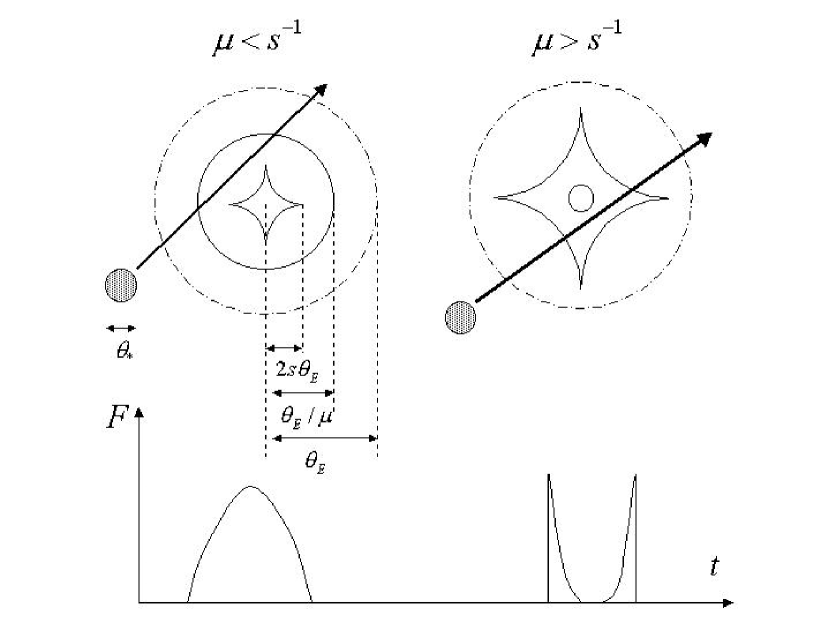
Figure 1: A schematic diagram for the two different cases of microlensing events: the point-mass lens limit ($\mu<s^{-1}$, left-hand side) and the caustic-crossing dominant limit ($\mu>s^{-1}$, right-hand side), where $\mu$ is the magnification required for detection and $s$ is the external shear at the lens location. The dot-dashed circles are the Einstein radius, and the solid circles have radii of $\theta_{E}/\mu$, and a source star with a radius $\theta_{*}$ must hit this region for its detection in the point-mass lens picture. On the other hand, the astroid-shaped curves are caustics, extending to $\sim 2s\theta_{E}$, and a source star must hit this region for its detection, in the caustic crossing limit. The corresponding light-curves are shown in the bottom, where the finite source size effect is assumed to be negligible. (For the condition of significant finite source size effect, see text.)

We should examine whether the caustics around the lens center generated by the external shear has a significant effect on the microlensing events. We use terms of ‘point-mass lens limit’ and ‘caustic-crossing limit’ when the caustic-crossing effect is negligible or not, respectively. The appropriate picture, point-mass lens or caustic crossing, is determined by the value of the shear $s$ and the magnification required for detection of a microlensed star, $\mu$. (See a schematic explanation in Fig. 1). When $\mu\ll s^{-1}$, the impact parameter (the minimum angular separation between a lens and a source star) required for detection is $\sim\theta_{E}/\mu$, which is much bigger than the size of the caustics, $2s\theta_{E}$. In this region outside the caustics, the magnification behavior is similar to that of an ideal point-mass lens without shear. On the other hand, when $\mu\gg s^{-1}$, a star crosses caustics before it reaches the radius of $\theta_{E}/\mu$, and hence the strong magnification by caustic crossing would dominate observable events. As mentioned above, the external shear is expected to be $\sim$ 0.02–0.2. Considering the distance modulus of the source cluster (38.73) and typical sensitivity of 8m-class telescopes ($m_{I}\sim 26$ at one hour exposure), we expect that the caustic crossing is appropriate in most cases, except for the brightest classes of source stars ($M_{I}\sim-10$) for which only a magnification of $\mu\sim 10$ is required for detection. In next subsections we will give formulations to estimate microlensing event rate for the both limits, and calculate the expected number of events. Then we examine, for typical events contributing to the event number, which limit applies in a supposed observation, which should be dependent on the lens mass considered.

In this paper we consider two modes of observation with total duration of $T_{\rm obs}$: (1) a consecutive observation during a night, typically $T_{\rm obs}\sim$ 6 hrs, and (2) a monitoring beyond the time scale of one night with arbitrary sampling time interval. The time resolution $t_{\rm res}$ would be minutes for the observing mode (1) for typical instruments, while it is $T_{\rm obs}/N_{\rm sample}$ for the mode (2), where $N_{\rm sample}$ is the total number of sampling (i.e., nights) during the total observing duration $T_{\rm obs}$.

2.2 Point-Mass Lens Limit ($\mu\ll s^{-1}$)

Let $f_{\rm lim,0}$ be the flux sensitivity limit with an exposure time $t_{\rm exp,0}$, for a given telescope. We also assume that the sensitivity limit scales as $f_{\rm lim}=f_{\rm lim,0}(t_{\rm exp}/t_{\rm exp,0})^{-1/2}$. First we consider the optimal lensing time scale and magnification to search for a microlensing event of a source star whose original luminosity is $L_{*}$, for the observing mode (1). The magnification required for detection at a flux level $f_{\rm lim}$ becomes $\mu=4\pi\tilde{d}_{\rm S}^{2}f_{\rm lim}/L_{*}$. For this magnification, the impact parameter between the source star and the lens must be smaller than $\theta<\theta_{E}/\mu$ when $\mu\gg 1$, and the time duration of lensing is given by $t_{\rm lens}=t_{\rm lens,E}\ \mu^{-1}$. Here, $t_{\rm lens,E}=\theta_{E}d_{L}/V$ is the Einstein-ring crossing time, and $V$ is the relative transverse velocity between the source and lens projected on the lens plane. The lensing duration must be longer than the supposed exposure time to detect an event, and hence this condition, $t_{\rm lens}\geq t_{\rm exp}$, results in the limiting magnification $\mu_{\lim}$ required, as:

$$\mu>\mu_{\lim}=\frac{t_{\exp,0}}{t_{\rm lens,E}}\left(\frac{4\pi\tilde{d}_{S}^{2}f_{\lim,0}}{L_{*}}\right)^{2}\ .$$ (3)

For the observing mode (2), the sensitivity is determined by the unit exposure time $t_{u}$ during one night (typically $t_{u}\sim$ 6 hrs), rather than by the lensing time scale that is longer than $t_{u}$. In this case, the limiting magnification is simply given as $\mu_{\lim}=4\pi\tilde{d}_{\rm S}^{2}f_{\rm lim,u}/L_{*}$, where $f_{\rm lim,u}=f_{\lim,0}(t_{u}/t_{0})^{-1/2}$ is the sensitivity limit for an exposure of the unit time scale.

We should also examine the finite source size effect. When the impact parameter $\theta_{E}/\mu$ becomes smaller than the size of source stars, i.e., $r_{*}>r_{\rm crit}\equiv\theta_{E}d_{S}/\mu$, this effect becomes significant, where $r_{*}$ is the size of stars.

To help the reader get a rough image of possible events, we show the values of representative quantities such as $t_{\rm lens}$, $\mu_{\lim}$, $r_{*}$ and $r_{\rm crit}$, for some values of lens mass $m_{\rm co}$ in Table 1. The observing mode (1) is assumed. For the treatment of stellar size and other parameters for the cluster-cluster system, see §3.1. These quantities could be very different for different source star luminosity, and this means that only stars in a relatively narrow range of luminosity would contribute to event rate, whose event time scale $t_{\rm lens}$ is matching the practical observing time scale.

The optical depth for such extremely magnified events is given by $\tilde{\tau}_{\rm co}=\tau_{\rm co}\mu_{\lim}^{-2}=f_{\rm co}m_{\rm co}^{-1}\Sigma(\theta)\pi\theta_{E}^{2}\mu_{\lim}^{-2}$, where $m_{\rm co}$ is the mass of compact lens objects, and $\Sigma(\theta)$ is the surface mass density of the lens cluster at the angle $\theta$ from the center. Then the total number of microlensing events detectable in one snapshot of the source cluster is given by

$$N_{\rm snapshot}(L_{*})dL_{*}=\int_{0}^{\theta_{\rm cl,S}}2\pi\theta d\theta S_{*}(\theta)\phi(L_{*})dL_{*}\tilde{\tau}_{\rm co}(\theta)\ ,$$ (4)

for source stars whose luminosity is in a range from $L_{*}$ to $L_{*}+dL_{*}$, where $S_{*}$ is the mean surface brightness of galaxies in the source cluster, $\phi$ the stellar luminosity function (LF) of source stars normalized by the total stellar luminosity, and $\theta_{\rm cl,S}$ the maximum angular extension of the source cluster. Here we implicitly assumed that the two clusters are perfectly aligned, which is a reasonable approximation for the A2152 system since the projected angular separation of the centers of the two clusters is comparable or even smaller than the typical core size of clusters. For a monitoring with duration $T_{\rm obs}$, the total expected number of events is then given by integrating over $L_{*}$,

$$N_{\rm event}=\int dL_{*}N_{\rm snapshot}(L_{*})\max(1,T_{\rm obs}/t_{\rm lens})\ .$$ (5)

In practice, the integration range over $L_{*}$ must be limited, since the lensing time scale must be reasonable with respect to the finite time resolution or duration of observation. (Note that $t_{\rm lens}\propto m_{\rm co}L_{*}^{2}$.) For the observing mode (1), we perform this integration when a condition on $t_{\rm lens}$, $5t_{\rm res}<t_{\rm lens}<T_{\rm obs}$, is satisfied, and for the observing mode (2), we set a condition $0.5T_{\rm obs}<t_{\rm lens}<2T_{\rm obs}$.

2.3 Caustic Crossing Limit ($\mu\gg s^{-1}$)

First we consider the event rate by lenses with a fixed value of shear $s$, and then we will integrate it over $s_{\rm co}$ with the probability distribution $p(s_{\rm co}|\tau_{\rm co})$. It can be shown that the magnification distribution function $P(\mu)$ becomes asymptotically the same with that of a point mass lens when $\mu\gg s^{-1}$, and behaves like $P(\mu)\propto\mu^{-3}$ (Schneider 1987; Kofman et al. 1997). It should be noted that not only the behavior ($\propto\mu^{-3}$) but also the angular area in the source plane for magnification larger than a given $\mu$ becomes the same as those of point mass lens in the limit of $\mu\gg s^{-1}$ (Kofman et al. 1997). Large magnification events should be dominated by caustic-crossing rather than cusps, since $P(\mu)$ around the cusps decreases with increasing $\mu$ as $\propto\mu^{-7/2}$, which is faster than the total $P(\mu)$ (Mao 1992). For a source crossing the caustics around a lens, the projected length of caustics on the source plane is $\sim 8s\theta_{E}$. Let $\theta_{\mu}$ be a characteristic width of the region along the caustics where magnification is larger than $\mu$. Then we expect that the area of this region, $\sim 8s\theta_{E}\theta_{\mu}$ should be equal to the equivalent area for a single point-mass lens, $\pi(\theta_{E}/\mu)^{2}$. Then we obtain

$$\theta_{\mu}\sim\frac{\pi\theta_{E}}{8s\mu^{2}}\ ,$$ (6)

which is related with the time duration for this magnification as:

$$t_{\mu}=\frac{\theta_{\mu}d_{L}}{V}\ .$$ (7)

These relations indicate that the light curve around the caustic crossing with a constant lens velocity is $\mu\propto t^{-1/2}$, as is well known for sources inside the caustics, while magnification suddenly drops when a source crosses and gets outside the caustics (e.g., Schneider & Weiß1986). Since the sensitivity of a telescope also roughly scales as $f_{\lim}\propto t^{-1/2}$, the signal-to-noise ratio should be roughly constant against the exposure time in a consecutive monitoring observation.

Therefore all stars brighter than a threshold luminosity can be detected by microlensing, when they pass a caustic. For observing mode (1), the magnified flux $f_{\mu}=\mu L_{*}/(4\pi\tilde{d}_{S}^{2})$ must be greater than the flux limit $f_{\lim}=f_{\lim,0}(t_{\mu}/t_{0})^{-1/2}$, and hence we obtain

$$L_{*,\min}(s)>4\pi\tilde{d}_{S}^{2}f_{\lim,0}\sqrt{\frac{8sVt_{0}}{\pi\theta_{E}d_{L}}}\ ,$$ (8)

which is independent of $t_{\mu}$ or the exposure time. In the case of observing mode (2), the sensitivity limit with an exposure of the unit observing time $t_{u}$ should be fainter than the magnified flux of stars with a lensing time scale of the total observing duration, i.e., $t_{\mu}=T_{\rm obs}$. Then we get

$$L_{*,\min}(s)>4\pi\tilde{d}_{S}^{2}f_{\lim,0}\sqrt{\frac{8sVt_{0}T_{\rm obs}}{\pi\theta_{E}d_{L}t_{u}}}\ .$$ (9)

Ignoring the finite source size effect, the maximum magnification $\mu_{\max}$ that can be observed is determined by the minimum time resolution, $t_{\rm res}$. Replacing $t_{\mu}$ by $t_{\rm res}$ in eqs. (6) and (7), we obtain:

$$\mu_{\max}=\sqrt{\frac{\pi\theta_{E}d_{L}}{8s\ t_{\rm res}V}}\ .$$ (10)

On the other hand, $\mu_{\max}$ may be limited by the finite source size effect. This effect becomes to be visible when the crossing time of stars, $r_{*}d_{L}/(Vd_{S})$, becomes larger than the time resolution $t_{\rm res}$. This condition can be written as:

$$r_{*}>r_{\rm crit}\equiv\frac{t_{\rm res}Vd_{S}}{d_{L}}\ .$$ (11)

These representative quantities, such as $M_{I,\max}$ corresponding to $L_{*,\min}$, $\mu_{\max}$, $r_{*}$ corresponding to $L_{*,\min}$, and $r_{\rm crit}$ are shown for some values of the lens mass, in Table 1. The observing mode (1) is assumed. It should be noted that $L_{*,\min}$ depends very weakly on the lens mass as $\propto m_{\rm co}^{1/4}$, and this suggests that this experiment has a sensitivity in a wide range of the lens mass, as we will see below. Although the finite source size effect seems too strong in all cases shown here, it should be noted that here we used rather small $t_{\rm res}=0.1$hrs as typically possible time resolution. We can increase $t_{\rm res}$ to, say, 1 hr for the observing mode (1) and 1 day for the mode (2). Then we may observe modest effect of finite source size, which does not seriously decrease detectability of events, but give important information about the stellar size that is useful to estimate $m_{\rm co}$.

The expected event number per one source star is calculated as the expected number of the caustic crossing, whose length is $\sim 8s\theta_{E}$ per microlens, as:

$$N_{1}(\theta,s_{\rm co})\ ds_{\rm co} = 8s(\theta)\ \theta_{E}\frac{V}{d_{L}}n_{\rm co}(\theta)\ p(s_{\rm co}|\tau_{\rm co})\ ds_{\rm co}\ T_{\rm obs}$$ (12)

$$= \frac{8s(\theta)\ VT_{\rm obs}\tau_{\rm co}(\theta)\ p(s_{\rm co}|\tau_{\rm co})\ ds_{\rm co}}{\pi\theta_{E}d_{L}}\ ,$$ (13)

for lenses whose $s_{\rm co}$ is in a range from $s_{\rm co}$ to $s_{\rm co}+ds_{\rm co}$, where the surface number density of lens is $n_{\rm co}=\tau_{\rm co}/(\pi\theta_{E}^{2})$. Note again that $s=s_{\rm co}+s_{\rm sm}$. Then the total event number is obtained by integrating over $s_{\rm co}$ and angular radius from the center of the cluster-cluster system, as:

$$N_{\rm event} = \int_{0}^{\theta_{\rm cl,S}}2\pi\theta d\theta S_{*}(\theta)\ \int ds_{\rm co}$$ (14)

$$\times N_{*}[L_{*,\min}\{s(\theta,s_{\rm co})\}]\ N_{1}[\theta,s_{\rm co}]\ ,$$

where $N_{*}(L_{*})$ is the number of stars brighter than $L_{*}$, i.e.,

$$N_{*}(L_{*})=\int_{L_{*}}^{\infty}\phi(L_{*}^{\prime})dL_{*}^{\prime}\ ,$$ (15)

which is normalized by the total stellar luminosity.

2.4 Image Separations and Time Delays

In the above formulations, we implicitly assumed that different lensed images cannot be resolved in observations, and the arrival time difference among them is negligible compared with observational time scales. Here we check this point. In the point-mass lens limit, there are two images separated by $\theta_{\rm sep}\sim 2\theta_{E}$, and time delay between the two can be calculated by the time delay function which is the sum of the geometrical and gravitational time delays (Narayan & Bartelmann 1995). To the third order of $1/\mu$ when $\mu\gg 1$, we find

$$\Delta t=\frac{d_{L}d_{S}}{c\ d_{LS}}\ \frac{\theta_{E}^{2}}{6\mu^{3}}\ .$$ (16)

In the caustic crossing limit, the separation of newly created two images when a source just gets inside the caustics is given by $\theta_{\rm sep}\sim\theta_{E}/\mu s$ ($\theta_{\rm sep}\rightarrow 0$ when the source approaches to the caustic), and time delay between the two images is given as

$$\Delta t\sim\frac{d_{L}d_{S}}{c\ d_{LS}}\ \frac{\theta_{E}^{2}}{\mu^{3}s^{2}}\ ,$$ (17)

which has a similar form to the point-mass lens limit (see, e.g., Schneider & Weiß 1986). As we will see later, the point-mass lens limit can be applied only for a small lens mass range of $m_{\rm co}\lesssim 0.1M_{\odot}$, and hence the image separation is practically unresolved by observations. The factor of $\mu^{-3}$ in $\Delta t$ indicates that the time delay is much shorter than observing time scales in all the lens mass range considered in this paper.

3 Event Rate Estimations

3.1 Input Parameters

We use a cluster total mass $M_{\rm cl}=10^{15}h^{-1}M_{\odot}$ for  the lensing cluster A2152 by a dynamical mass estimate within $R_{\rm cl,L}=d_{L}\theta_{\rm cl,L}=1.6h^{-1}$ Mpc (Barmby & Huchra 1998). The mass of the source cluster is uncertain, but it seems more massive than A2152 (Blakeslee 2001). Here we use the same mass and radius with those of A2152. The velocity dispersion of A2152 is $\sim$700 km/s, and probably it has a comparable transverse peculiar velocity of bulk motion. Therefore, we use $V$ = 1000 km/s as a plausible value.

The density profiles of lens objects in the lens cluster and source stars in the source cluster must be specified. For the stellar density profile in the source cluster, we assume the King profile (King 1962) ($S_{*}\propto[1+(\theta/\theta_{\rm core})^{2}]^{-1}$), which is the most widely used for the number distribution of galaxies. We also assume a core size of $R_{\rm core}=0.09h^{-1}$Mpc in the King profile. We consider observations in the $I$ band, and use a mass-to-light ratio of the source cluster to normalize the surface brightness $S_{*}$, as $M_{\rm cl}/L_{\rm cl,I}=180h(M_{\odot}/L_{I,\odot})$, which is converted from $M/L_{V}$ for rich clusters in Bahcall & Comerford (2002) using a typical color of cluster galaxies, $V-I=1.6$. In this paper we use the same King profile also for lens objects in the lens cluster; this is reasonable when the lens objects are tracing the stellar mass in the cluster, as expected for intracluster stars. On the other hand, the Navarro, Frenk, & White (1997, hereafter NFW) density profile may be appropriate for non-interacting dark matter (see also Bartelmann 1996 for the projected surface density profile of NFW). If we use the NFW profile [$\rho\propto(cr/R_{\rm cl,L})^{-1}(1+cr/R_{\rm cl,L})^{-2}$] for the lens cluster with a typical concentration parameter of $c=5$ (e.g., Allen, Ettori, & Fabian 2001), we find that the microlensing probability is reduced by a factor of about 2 compared with the King profile. Finally, we use the singular isothermal sphere with a softened core (eq. 2), having the same core radius with the King profile, to calculate the shear of smoothly distributed mass. It is partially for computational simplicity, but also a reasonable treatment for intracluster gas.

The LF of source stars must be specified. Here we try two LFs for disk and elliptical galaxy populations. For disk galaxies, we used the $I$ band LF of Mamon & Soneira (1982). For elliptical galaxies or stellar population in bulges, we use the LF of our Galaxy bulge presented in Terndrup, Frogel, & Whitford (1990) showing a cut-off of giant stars brighter than $M_{I}=-4$, corresponding to the tip of the red giant branch. The elliptical/bulge LF has some structure around $M_{I}\sim 0$ due to the red clump stars. The stellar size as a function of stellar luminosity $M_{I}$ is necessary to check the finite source size effect. The approximate radius of stars, $r_{*}$, is calculated by the bolometric luminosity and the effective temperature ($r_{*}\propto L_{*,\rm bol}^{1/2}T_{\rm eff}^{-2}$). According to Mamon & Soneira (1982), we consider five subclasses of stellar populations, i.e., two supergiant classes (Ia and Ib), bright giants (II), giants (III), and main sequence (V), which are dominant in different ranges of $M_{I}$ with an increasing order, and the borders between these are $M_{I}\sim-8,-6,-4,$ and 0. The $(V-I)$ versus $M_{I}$ relation for these subclasses is also given in Mamon & Soneira (1982), from which we infer the spectral type, effective temperature, and bolometric corrections in Zombeck (1990). The LF, $(V-I)$ color, and stellar radius are shown in Fig. 2.

3.2 Results

Here we calculate the expected event rate supposing an observation by Subaru/Suprime-Cam, whose sensitivity is $m_{\lim,0,I}=26.0$ (S/N=5) at $t_{\exp,0}$= 1 hr. In the point-mass lens approximation, we require a signal-to-noise of $S/N>10$ and $S/N>5$ for the observing modes (1) and (2), respectively. The higher $S/N$ is required for the observing modes (1) to assure sufficient $S/N$ to construct a microlensing light curve. On the other hand, in the caustic-crossing limit, we require a signal-to-noise of $S/N>5$ and $S/N>3$, respectively. The lower $S/N$ is adopted because the strong magnification near the caustic-crossing is expected to increase total effective $S/N$ compared with the point-mass lens limit. (However, when the finite source size effect is significant, this may not apply. See below.)

In Figures 3 and 4, we show the expected limit on $f_{\rm co}$ obtained by an observation using 10 nights, i.e., 10 times repetition of the observing mode (1) with $T_{\rm obs}=6$ hrs and $t_{\rm res}=0.1$ hrs, in the limits of point-mass lens and caustic crossing, respectively. Figures 5 and 6 are the same, but for the observing mode (2) using 10 nights, with $T_{\rm obs}=10$ days and $N_{\rm sample}=10$. In all these four figures, the limits on $f_{\rm co}$ are shown in the upper panels as a function of various lens mass. In the lower panels, we plot the mean of $s\mu$, $r_{*}$, and $M_{I}$ for events contributing to $N_{\rm event}$. The calculation in the point-mass lens or caustic-crossing limits is valid only when $s\mu\lesssim 1$ or $\gtrsim 1$, respectively. Here, the limit on $f_{\rm co}$ is defined as the value where the total expected event number, $N_{\rm event}$ is unity. It should be noted that $N_{\rm event}\propto f_{\rm co}$ in the point-mass lens limit, while this relation holds only approximately in the caustic-crossing limit, since a change of $f_{\rm co}$ would change the shear $s$. Equations 8, 9, 13, and 14 indicate that this relation depends on the shape of LF, and $N_{\rm event}\propto f_{\rm co}$ is exactly valid only when $N_{*}(L_{*})\propto L_{*}^{-2}$, which is a roughly correct approximation in a range of $M_{I}\lesssim-4$.

The point-mass lens approximation is valid only when $\langle s\mu\rangle\lesssim 1$, while the caustic-crossing limit is appropriate only when $\langle s\mu\rangle\gtrsim 1$, where $\langle x\rangle$ represents a mean of the quantity $x$ over all detectable events. The transition between the two limits occurs at $\langle\mu s\rangle\sim 1$, which is at $m_{\rm co}\sim 10^{-5}M_{\odot}$ in the observing mode (1) and at $m_{\rm co}\sim 0.1M_{\odot}$ in the observing mode (2), respectively. At these transition points, both the limits are approximately valid and hence the event rate predictions should agree with each other. Indeed the two predictions agree at the transition lens mass scale, providing a support for the validity of our formulations and calculations.

Most behavior of the $f_{\rm co}$ limit as a function of $m_{\rm co}$ can be understood as follows. A trend easily seen is that typical source star luminosity contributing to event rate becomes smaller with increasing lens mass. In the point-mass limit, the duration of strong magnification required for detection is $t_{\rm lens}\propto t_{\rm lens,E}/\mu_{\lim}\propto m_{\rm co}L_{*}^{2}$. Since we are supposing 10 nights duration of observation, and the detectable time scale is limited by this specific time scale. Therefore $\langle L_{*}\rangle\propto m_{\rm co}^{-1/2}$. In the caustic-crossing limit, on the other hand, there is the minimum source star luminosity $L_{*,\min}$ for detectable events, and hence $\langle L_{*}\rangle\propto L_{*,\min}\propto\theta_{E}^{-1/2}\propto m_{\rm co}^{-1/4}$. This is why the typical source star luminosity and limits on $f_{\rm co}$ are less sensitive to $m_{\rm co}$ in the caustic-crossing limit, than the point-mass limit. The event rate in the point-mass lens limit scales as

$$R_{\rm event}\propto\frac{dN_{*}(\langle L_{*}\rangle)}{d\log L_{*}}\ \tilde{\tau}_{\rm co}\propto\frac{dN_{*}(\langle L_{*}\rangle)}{d\log L_{*}}\ \langle L_{*}\rangle^{2}\ ,$$ (18)

per logarithmic stellar luminosity interval. On the other hand, the event rate in the caustic-crossing limit scales as $\propto N_{*}(\langle L_{*}\rangle)\ \theta_{E}^{-1}\propto N_{*}(\langle L_{*}\rangle)\ \langle L_{*}\rangle^{2}$. These two have the same dependence on $L_{*}$, and hence the curves of $f_{\rm co}$ limit in Figs. 3–6 can be understood as inverted stellar luminosity function per logarithmic interval which is multiplied by $L_{*}^{2}$. Since $dN_{*}/d\log L_{*}\propto N_{*}(L_{*})\propto L_{*}^{-2}$ at $M_{I}\lesssim-4$, the limit on $f_{\rm co}$ is roughly constant, but it becomes weaker with decreasing stellar luminosity at $M_{I}\gtrsim-4$ because of the change of the luminosity function slope.

The finite source size effect could be significant in the observing mode (1). (Note that the finite source size effect is not taken into account in the event rate estimates presented here.) Although $r_{*}/r_{\rm crit}$ appears to be much larger than unity in the caustic-crossing limit (Fig. 4), this partly comes from the use of small $t_{\rm res}$ = 0.1 hrs in eq. (11), as mentioned in §2.3. Since the light curve of caustic crossing is $f\propto t^{-1/2}$ for a point source, the signal-to-noise ratio does not change much when we change the monitoring time scale of events. If we choose a longer time scale, the finite source size effect becomes less significant. We will be able to increase $t_{\rm res}$ up to a few hours during a night, and hence the finite source size effect should not severely suppress the detectable event rate estimated here, especially for larger $m_{\rm co}$. The finite source size effect is mostly insignificant for the observing mode (2).

To summarize, these results indicate that monitoring of the cluster-cluster system using 10 nights of a wide-field 8m-class telescope can probe possible intracluster compact objects, with a sensitivity to the mass fraction in the total cluster mass as $f_{\rm co}\sim$ 1–3 % at $m_{\rm co}\sim 10^{-5}$–$10^{8}M_{\odot}$ in the observing mode (1), and $f_{\rm co}\sim$ 3–10 % at $m_{\rm co}\sim 10^{-3}$–$10^{10}M_{\odot}$ in the observing mode (2). The sensitivity in the observing mode (1) might be somewhat reduced by the finite source size effect, but we expect that it is not significant.

4 Discussion

A weak point of pixel lensing is that there is a degeneracy of lens parameters due to the lack of information of the source star luminosity. Even if we assume the transverse lens velocity as $V\sim 1000$ km/s, the lens mass cannot be determined if we do not know the source luminosity. It is not easy to break this degeneracy, but it might be possible if the color of microlensing events is measured. Elliptical galaxies have only old stellar populations and there is a sharp cut off of the stellar luminosity function at the tip of the red giant branch, where the $V-I$ color of stars becomes rapidly redder at almost constant $M_{I}$ on the color-magnitude diagram (e.g., Jablonka et al. 1999). Therefore, when a microlensing event with very red color is observed in an elliptical galaxy, it is very likely that the source star has an absolute magnitude of $M_{I}\sim-4$, making the lens mass estimate possible. When the finite source size effect is seen in an observed light curve, it also gives additional information on the apparent stellar size, which can be used to break the degeneracy (Gould 1997; Sumi & Honma 2000).

It is important to discriminate the microlensing events from other astronomical transient sources. In addition to the features generally used in microlensing searches, i.e., characteristic light curves and achromatic behavior, there are two expected signatures that are unique for this system: 1) more events are expected for stars in the source cluster $(z=0.13)$ rather than in the lens cluster $(z=0.04)$, and 2) the event distribution is even more concentrated to the cluster center than the matter distribution in clusters, since the lensing probability is proportional to the product of the surface densities of the source and lens clusters.

Another interesting possibility that may be useful for discrimination and breaking the degeneracy is repetition of caustic crossings. When a source star crosses the astroid-shaped caustics of a lens, typically two, and sometimes even more caustic-crossings are expected. The time interval of repetition is roughly given as

$$t_{\rm rep}\sim\frac{2s\theta_{E}d_{L}}{V}=3.0\times 10^{6}\left(\frac{m_{\rm co}}{M_{\odot}}\right)^{1/2}\left(\frac{s}{0.01}\right)\ \rm s\ .$$ (19)

Therefore, repetition of caustic-crossings is expected during the observing duration $T_{\rm obs}\sim$ 10 days, if the lens mass is smaller than $m_{\rm co}\lesssim 0.1M_{\odot}$. Such repeating events at the same location in a host galaxy with characteristic light-curves of caustic crossing would be a good evidence for microlensing, and also provide independent information of $\theta_{E}$, and hence, the lens mass.

In the microlensing experiments towards the Magellanic Clouds, the self-lensing event rate by stars in MCs is comparable to those by lenses in the Galactic halo. This has been one of the major causes of the controversial interpretations of the microlensing events to MCs (e.g., Jetzer, Mancini, & Scarpetta 2002). The situation is similar also for the pixel lensing experiments towards the M31 galaxy (Paulin-Henriksson et al. 2002) or M87 in the Virgo cluster (Gould 1995). However, in the cluster-cluster system, the lens cluster is located far from both the source system and the observer, and the lensing events by compact objects in the lens cluster should dominate those in the source cluster, because of the larger Einstein radius. In fact, the optical depth to the self-lensing does not depend on the distance, but is simply $\tau\sim(\upsilon_{\rm vir}/c)^{2}\sim 10^{-7}$–$10^{-6}$ which is much smaller than that of the cluster-cluster system, where $\upsilon_{\rm vir}\sim 200$ km/s is the virial velocity of the stellar system.

We should examine that the microlensing event rate in the cluster-cluster system are sufficiently higher than contaminating events by stars or lenses in the field outside the source and lens clusters. First we consider the case that the stars in the source cluster are lensed by compact objects outside the lens cluster (i.e., in the field). A comparison can be made in terms of the optical depth; taking the matter density of the universe to be $\Omega_{M}=0.3$, we found that the field optical depth to the distance $d_{S}$ is $4.2\times 10^{-3}$, which is more than 10 times smaller than that of the lens cluster, 0.1–0.2, which is a weighted mean with the source star surface density. Secondly, we consider the case where stars in field galaxies behind the lens cluster are lensed by compact objects in the lens cluster. Assuming a constant stellar to total mass ratio for clusters and fields, about a third of the stellar mass of the source cluster is included in the field galaxies in the cone made by the observer and a projected surface area of the source cluster. For these field stars, mean optical depth of the lens cluster is $\sim 0.03$ assuming the King profile. Combining these factors, it can be concluded that the events by source stars in the field is more than 10 times less frequent than those by stars in the source cluster.

Apart from microlensing, the mean steady flux of stars and galaxies in the background cluster are also magnified by macrolensing, i.e., gravitational lensing effect of the mass distribution on the cluster scale. This effect makes less luminous stars detectable than we considered by the above formulations, and hence increasing the event rate. According to the modeling of Blakeslee et al. (2001), we expect that macrolensing magnification is greater than a factor of 1.5 in the central 30” radius region of A2152, for background sources at $z\sim 0.13$. The magnification becomes more than 10 within the 10” radius. These regions are not significant compared with the total cluster field, but somewhat comparable with the core regions of these clusters. Since a considerable fraction of projected mass is included in the core regions, this effect could be significant and may be observed as even stronger concentration of events to the core regions, than expected from the product of surface densities of the source and lens clusters. On the other hand, it should also be noted that the macrolensing effect must be corrected when one estimates the mean galaxy surface brightness, $S_{*}$, from observed galaxy distributions.

When a microlensing event occurred in a very high surface-brightness region of a galaxy, the sensitivity to transient point sources could be effectively reduced. However, generally ground-based observations are limited by the sky background rather than surface brightness of galaxies. Assuming a sky background of 19.5 mag arcsec^-2 in the $I$ band for a moderately dark sky at Mauna Kea, we estimated about 74% of the galactic light of the source cluster at $z=0.13$ is coming from a region whose surface brightness is lower than the sky background, by using the local galaxy luminosity function, the mean luminosity-size relation of galaxies, and surface brightness profiles presented in Totani & Yoshii (2000). Here, we assumed a condition of 1 arcsec seeing, and the morphological type mix is taken to be 70% for the ellipticals and 30% for spirals. Therefore, effective reduction of the sensitivity due to high surface brightness of host galaxies is not a serious problem.

5 Astrophysical Implications

The sensitivity of $f_{\rm co}\sim$ a few percent in a range of $m_{\rm co}\sim 10^{-5}$–$10^{10}M_{\odot}$ is sufficiently good as a probe for the nature of dark matter; we could detect or reject any compact objects in this mass range as the dominant component of the dark matter in galaxy clusters. It should be noted that this mass range fills up the “desert” of the constraints on $\Omega_{M}$ in the form of compact objects: $m_{\rm co}\sim 10$–$10^{5}M_{\odot}$, which has hardly been constrained by past observations. Microlensing searches in nearby galaxies or quasar variability have constrained at $m_{\rm co}\lesssim 10M_{\odot}$, while millilens searches for radio quasars or echos of gamma-ray bursts constrained at $m_{\rm co}\gtrsim 10^{5}M_{\odot}$ (Narayan & Bartelmann 1995; Nemiroff et al. 2001; Wilkinson et al. 2001, and see Wambsganss 2002 for the latest review).

Hawkins (1993, 1996) claimed that variability seen in high-$z$ quasars is due to the microlensing action of Jupiter-mass compact objects distributed cosmologically, whose density is enough to explain a significant fraction of the dark matter. However, this claim has been questioned by a number of authors (e.g., Baganoff & Malkan 1995; Alexander 1995). Some observations of strongly lensed quasars have been used to exclude this possibility (Schmidt & Wambsganss 1998; Wyithe, Webster, & Turner 2000), although it also depends on assumed quasar sizes. The latest data of EROS project also seem to have excluded this possibility (Lasserre et al. 2000). Anyway, this experiment would provide another independent test for this controversial claim.

If MACHOs exist in the intracluster space with a similar mass fraction ($\sim$ 20%) suggested by the MACHO collaboration (Alcock et al. 2001), the cluster-cluster microlensing search should find about 1–10 events. However, it should be noted that the mass-to-light ratio of clusters is much larger than that of the Galactic halo. If the abundance of MACHOs scales with luminous matter, we expect that the intracluster MACHO mass fraction is much smaller than in the Galaxy. Some observations suggest that MACHOs may be white dwarfs (Ibata et al. 2000; Oppenheimer et al. 2001), but if 20% of the total cluster mass is in the form of white dwarfs, and the matter content in the cluster system is the same as that of the whole universe, almost all of the cosmic baryons predicted by the big-bang nucleosynthesis [$\Omega_{B}\sim 0.02h^{-2}=0.07h^{-2}\Omega_{M}(\Omega_{M}/0.3)^{-1}$, Burles & Tytler (1998)] must be locked up in white dwarfs. Such a case would easily violate the constraint coming from the cosmic background radiation (CBR) in optical and infrared bands (Madau & Pozzetti 2000).

On the other hand, there are a few recent reports by independent groups for detections of the near-infrared CBR (Matsumoto 2000; Cambrésy et al. 2001; Wright 2001), and the reported flux is by a factor of a few higher than the flux integration of galaxy counts in the same band, which is difficult to explain by normal galactic light even if the incompleteness of galaxy surveys and the cosmological surface brightness dimming of galaxies are taken into account (Totani et al. 2001). Though the discrepancy may be solved if there are some systematic errors in processes of diffuse CBR measurement, e.g., subtraction of the zodiacal light (Wright & Johnson 2001), it is also possible that the CBR excess is due to exotic extragalactic sources that are very different from normal galaxies. If white dwarfs that were formed at very high redshift are responsible for this excess ($I\sim 30\rm nW\ m^{-2}sr^{-1}$), the mass density of white dwarfs and their progenitors would be about 2% and 10% of the nucleosynthetic baryons, respectively, assuming that 80% of baryons in progenitors is returned into interstellar space (Madau & Pozzetti 2000). Therefore, a plausible fraction of such white dwarfs in the total cluster mass is only $\sim$ 0.2%. It is not impossible, but rather difficult to detect these objects by the cluster-cluster microlensing experiment, unless a large number of nights are available.

Another possible source of this excess of CBR is the first generation stars at redshift $z\sim 10$, whose UV and optical light is redshifted to the near infrared band (Santos, Bromm, & Kamionkowski 2002; Schneider et al. 2002; Salvaterra & Ferrara 2002). Recent theoretical studies on the formation of primordial stars strongly indicate that they are very massive ($\gtrsim 100M_{\odot}$), and a majority of them might eventually evolve into massive black holes without ejection of any amount of heavy elements. Then, a major episode of the first-generation star formation is possible before the interstellar matter is polluted by metals and normal star formation begins (Schneider et al. 2002). Assuming a conversion efficiency from the rest mass to radiation energy that is similar to normal stars, a mass comparable with the present-day stars [$\Omega_{*}\sim 0.0024h^{-1}$, Fukugita, Hogan, & Peebles (1998)] must have been locked in the first generation stars and then their remnant black holes with $M\gtrsim 100M_{\odot}$, to explain the CBR excess. If such black holes are diffusely distributed in intracluster medium, the cluster-cluster microlensing search might detect them.

It is expected that there is a diffuse population of intracluster stars that are stripped from galaxies by interactions with other galaxies or intracluster gas. Observations of diffuse optical light, intracluster planetary nebulae, and red giant stars indicate that the amount of stellar light from such intracluster stars is 10–50% of the total light from galaxies in clusters, though these estimates are still highly uncertain (e.g., Vílchez-Gómez, Pelló, & Sanahuja 1994; Gonzalez et al. 2000; Arnaboldi et al. 2002; Durrell et al. 2002; Okamura et al. 2002). As shown above, about one percent of $\Omega_{M}$ is locked in stars in the universe, and this fraction is probably even higher in clusters of galaxies because of larger fraction of elliptical galaxies. Therefore, if the amount of intracluster stars is comparable with that of stars in member galaxies, the microlensing search of the Hercules supercluster might detect them, providing a completely independent information for intracluster stars.

The author is deeply indebted to B. Paczyński for many inspiring conversations. He would also like to thank M. Chiba, E. Komatsu, S. Mao, J. Ostriker, T. Sumi, J. Wambsganss, and M. Kubota for useful information and discussions. He has been financially supported in part by the JSPS Postdoctoral Fellowship for Research Abroad.

Table 1: Quantities for Some Representative Cases

		Point-Mass Lens Limit						Caustic Crossing Limit
$m_{\rm co}[M_{\odot}]$	$\theta_{E}[\mu{\rm as}]$	$M_{I}$	$t_{\rm lens}$[hrs]	$\mu_{\lim}$	$r_{*}[R_{\odot}]$	$r_{\rm crit}[R_{\odot}]$		$M_{I,\max}$	$\mu_{\max}$	$r_{*}[R_{\odot}]$	$r_{\rm crit}[R_{\odot}]$
$10^{-6}$	$5.8\times 10^{-3}$	$-10$	11	3.7	400	190		$-8.75$	$1.3\times 10^{2}$	200	1.7
$10^{-3}$	$1.8\times 10^{-1}$	$-7$	44	29	150	770		$-6.9$	$7.1\times 10^{2}$	150	1.7
$1$	5.8	$-3$	29	$1.4\times 10^{3}$	40	500		$-5.0$	$4.0\times 10^{3}$	50	1.7
$10^{3}$	$1.8\times 10^{2}$	1	19	$6.8\times 10^{4}$	3	330		$-3.1$	$2.2\times 10^{4}$	30	1.7
$10^{6}$	$5.8\times 10^{3}$	5	12	$3.3\times 10^{6}$	0.9	220		$-1.3$	$1.3\times 10^{5}$	10	1.7
$10^{9}$	$1.8\times 10^{5}$	9	7.6	$1.7\times 10^{8}$	0.4	140		$0.6$	$6.8\times 10^{5}$	4	1.7

Figure 2: The luminosity function (LF), $(V-I)$ color, and radius of source stars as a function of $I$ magnitude. Five different classes of stars [supergiants (Ia and Ib), bright giants (II), giants (III), and main sequence (V)] are assumed to be dominant, depending on the magnitude, as shown in the top panel. The solid line in the top panel is LF in spiral galaxies, while the dashed line is that in elliptical galaxies having old stellar populations.

Figure 3: The sensitivity to the mass fraction $f_{\rm co}$ of compact objects in the total cluster mass, in the limit of point-mass lens approximation (valid only when $s\mu\lesssim 1$), by 10 times repetition of consecutive monitoring during a night (6 hrs) with observing mode (1). Top panel: the limit on $f_{\rm co}$ as a function of the lens mass, assuming the stellar luminosity function in spiral galaxies (dashed line), in elliptical galaxies (dot-dashed line), and the weighted mean with relative proportions of 30% for spirals and 70% for ellipticals (solid line). Bottom panel: the mean values of original absolute $I$ magnitude of source stars ($M_{I}$), product of magnification and shear ($s\mu$), and the ratio of the stellar size to the critical size for finite source size effect ($r_{*}/r_{\rm crit}$).

Figure 4: The same as Fig. 3, by 10 times repetition of consecutive monitoring during a night (6 hrs) with observing mode (1), but in the limit of the caustic-crossing approximation, which is valid only when $s\mu\gtrsim 1$.

Figure 5: The same as Fig. 3, but by the observing mode (2) with $T_{\rm obs}=10$ days and $N_{\rm sample}=10$. This figure is assuming the single lens limit, which is valid only when $s\mu\lesssim 1$.

Figure 6: The same as Fig. 3, but by the observing mode (2) with $T_{\rm obs}=10$ days and $N_{\rm sample}=10$, and in the limit of the caustic-crossing approximation, which is valid only when $s\mu\gtrsim 1$.

References

- (1)
- (2) Alcock, C. et al. 2001, ApJ, 542, 281
- (3)
- (4) Alexander, T. 1995, MNRAS, 274, 909
- (5)
- (6) Allen, S.W., Ettori, S., & Fabian, A.C. 2001, MNRAS, 324, 877
- (7)
- (8) Ansari, R. et al. 1997, A&A, 324, 843
- (9)
- (10) Arnaboldi, M. et al. 2002, AJ, 123, 760
- (11)
- (12) Baganoff, F.K., & Malkan, M.A. 1995, ApJ, 444, L13
- (13)
- (14) Bahcall, N.A. & Comerford, J.M. 2002, ApJ, 565, L5
- (15)
- (16) Baillon, P., Bouquet, A., Giraud-Héraud, Y., & Kaplan, J. 1993, A&A, 277, 1
- (17)
- (18) Barmby, P. & Huchra, J.P. 1998, ApJ, 115, 6
- (19)
- (20) Bartelmann, M. 1996, A&A, 313, 697
- (21)
- (22) Blakeslee, J.P., Metzger, M.R., Kuntschner, H., & Côte, P. 2001, ApJ, 121, 1
- (23)
- (24) Blakeslee, J.P. 2001, to appear in The Dark Universe: Matter, Energy, and Gravity, STScI Symposium, April 2001, Ed. M. Livio (astro-ph/0108253)
- (25)
- (26) Burles, S. & Tytler, D. 1998, ApJ, 499, 699
- (27)
- (28) Calchi Novati, S. et al. 2002, A&A, 381, 848
- (29)
- (30) Cambrésy, L., Reach, W.T., Beichman, C.A., Jarret, T.H. 2001, ApJ, 555, 563
- (31)
- (32) Chang, K. & Refsdal, S. 1979, Nature, 282, 561
- (33)
- (34) Chang, K. & Refsdal, S. 1984, A&A, 132, 168 (E) 139, 558
- (35)
- (36) Crotts, A.P.S. 1992, ApJ, 399, L43
- (37)
- (38) Crotts, A.P.S. & Tomaney, A.B. 1996, ApJ, 473, L87
- (39)
- (40) Durrell, P.R., Ciardullo, R., Feldmeier, J.J., Jacoby, G.H., & Sigurdsson, S. 2002, ApJ, 570, 119
- (41)
- (42) Fukugita, M., Hogan, C.J., & Peebles, P.J.E. 1998, ApJ, 503, 518
- (43)
- (44) Gonzalez, A.H., Zabludoff, A.I., Zaritsky, D., & Dalcanton, J.J. 2000, ApJ, 536, 561
- (45)
- (46) Gould, A. 1995, ApJ, 455, 44
- (47)
- (48) Gould, A. 1996, ApJ, 470, 201
- (49)
- (50) Gould, A. 1997, ApJ, 480, 188
- (51)
- (52) Hawkins, M.R.S. 1993, Nature, 366, 242
- (53)
- (54) Hawkins, M.R.S. 1996, MNRAS, 278, 787
- (55)
- (56) Ibata, R., Irwin, M.J., Bienaymé, O., Schlolz, R., & Guibert, J. 2000, ApJ, 532, L41
- (57)
- (58) Jablonka, P., Bridges, T.J., Sarajedini, A., Meylan, G., Maeder, A., & Meynet, G. 1999, ApJ, 518, 627
- (59)
- (60) Jetzer, Ph., Mancini, L., & Scarpetta, G. 2002, A&A, 393, 129
- (61)
- (62) King, I. 1962, AJ, 67, 471
- (63)
- (64) Kofman, L., Kaiser, N., Hoi Lee, M., & Babul A., 1997, ApJ, 489, 508
- (65)
- (66) Lasserre, T. et al. 2000, A&A, 355, L39
- (67)
- (68) Lewis, G.F., Ibata, R.A., & Wyithe, J.S.B. 2000, ApJ, 542, L9
- (69)
- (70) Lewis, G.F., & Ibata, R.A. 2001, ApJ, 549, 46
- (71)
- (72) Madau, P. & Pozzetti, L. 2000, MNRAS, 312, L9
- (73)
- (74) Mamon, G.A. & Soneira, R.M. 1982, ApJ, 255, 181
- (75)
- (76) Mao, S. 1992, ApJ, 389, 63
- (77)
- (78) Matsumoto, T. 2000, in proceedings of the IAU symposium 204, ‘The Extragalactic Infrared Background and its Cosmological Implications’, ed. M. Harwit.
- (79)
- (80) Nakamura, T. & Nishi, R. 1998, Prog. Theo. Phys. 99, 963
- (81)
- (82) Narayan, R. & Bartelmann, M. 1995, in Formation of Structure in the Universe, Proceedings of the 1995 Jerusalem Winter School, ed. A. Dekel and J.P. Ostriker (Cambridge University Press)
- (83)
- (84) Navarro, J.F., Frenk, C.S., & White, D.M. 1997, ApJ, 490, 493
- (85)
- (86) Nemiroff, R.J., Marani, G.F., Norris, J.P., Bonnel, J.T. 2001, Phys. Rev. Lett. 86, 580
- (87)
- (88) Nityananda, R. & Ostriker, J. P. 1984, Journal of Astrophys. Astron. 5, 235
- (89)
- (90) Okamura, S. et al. 2002, PASJ in press, astro-ph/0211352
- (91)
- (92) Oppenheimer, B.R., Hambly, N.C., Digby, A.P., Hodgkin, S.T., Saumon, D. 2001, Sci., 292, 698
- (93)
- (94) Paczyński, B. 1986, ApJ, 304, 1
- (95)
- (96) Paulin-Henriksson, S. et al. 2002, preprint, astro-ph/0207025
- (97)
- (98) Riffeser, A. et al. 2001, A&A, 379, 362
- (99)
- (100) Salvaterra, A. & Ferrara, A. 2002, MNRAS in press, astro-ph/0210331
- (101)
- (102) Santos, M.R., Bromm, V., Kamionkowski, M. 2002, MNRAS in press (astro-ph/0111467)
- (103)
- (104) Schmidt, R. & Wambsganss, J. 1998, A&A, 335, 379
- (105)
- (106) Schneider, P., & Weiß, A. 1986, A&A, 164, 237
- (107)
- (108) Schneider, P. 1987, ApJ, 319, 9
- (109)
- (110) Schneider, R., Ferrara, A., Natarajan, P., & Omukai, K. 2002, ApJ, 571, 30
- (111)
- (112) Sumi, T. & Honma, M. 2000, ApJ, 538, 657
- (113)
- (114) Tadros, H., Warren, S., & Hewett, P. 1998, New. Astron. 42, 115
- (115)
- (116) Terndrup, D.M., Frogel, J.A., & Whitford, A.E. 1990, ApJ, 357, 453
- (117)
- (118) Totani, T. & Yoshii, Y. 2000, ApJ, 540, 81
- (119)
- (120) Totani, T., Yoshii, Y., Iwamuro, F., Maihara, T., & Motohara, K. 2001, ApJ, 550, L137
- (121)
- (122) Turner, E.L. & Umemura, M. 1997, ApJ, 483, 603
- (123)
- (124) Vílchez-Gómez, R., Pelló, R., & Sanahuja, B. 1994, A&A, 283, 37
- (125)
- (126) Walker, M.A. & Ireland, P.M. 1995, MNRAS, 275, L41
- (127)
- (128) Wambsganss, J., Paczyński, B., & Schneider, P. 1990, ApJ, 358, L33
- (129)
- (130) Wambsganss, J. 2002, in ‘Where’s the Matter? Tracing Bright and Dark Matter with the New Generation of Large Scale Surveys’, Eds. M. Treyer & L. Tresse (astro-ph/0207616)
- (131)
- (132) Wilkinson, P.N. et al. 2001, Phys. Rev. Lett. 86, 584
- (133)
- (134) Wright, E. L. 2001, ApJ, 553, 538
- (135)
- (136) Wright, E. L. & Johnson, B. D. 2001, submitted to ApJ, astro-ph/0107205
- (137)
- (138) Wyithe, J. S. B., Webster, R. L., & Turner, E. L. 2000, MNRAS, 315, 51
- (139)
- (140) Zombeck, M.V. 1990, Handbook of Space Astronomy and Astrophysics, Cambridge Univ. Press.
- (141)