Photometric Properties of Galaxy Population in the Cluster EIS 0048-2942 at $\mathrm{z\sim 0.64}$

Deep photometric data in the V-, R-, I-, z- and K-bands for the cluster of galaxies EIS 0048-2942 are used to investigate the properties of the galaxy populations at $\mathrm{z\sim 0.64}$ in a field of $\mathrm{2.5\times 2.5\leavevmode\nobreak\ Mpc^{2}}$. The sample of candidate cluster members ($\mathrm{N=171}$) is selected by the photometric redshift technique and is complete up to $\mathrm{I=22.5}$. Galaxies were classified as spheroids and disks according to the shape of the light profile in the I-band, as parametrized by the Sersic index. In both optical and NIR, spheroids define a sharp colour-magnitude sequence, whose slope and zero points are consistent with a high formation redshift ($\mathrm{z_{f}>2}$). The disk population occupies a different region in the colour-magnitude diagram, having bluer colours with respect to the red sequence. Interestingly, we find some level of mixing between the properties of the two classes: some disks lie on the colour-magnitude sequence or are redder, while some spheroids turn out to be bluer. The spatial distribution of cluster galaxies show a clumpy structure, with a main over-density of radius $\mathrm{\sim 0.5\leavevmode\nobreak\ Mpc}$, and at least two other clumps distant $\mathrm{\sim 1\leavevmode\nobreak\ Mpc}$ from the center. The various sub-structures are mostly populated by the red galaxies, while the blue population has an almost uniform distribution. The fraction of blue galaxies in EIS 0048-2942 is $\mathrm{f_{B}=0.11\pm 0.07}$. This is much lower than what expected on the basis of the Butcher-Oemler effect at lower redshifts.

1 Introduction

Since 1978 (Butcher & Oemler 1978a , 1978b ), several studies have been fruitfully undertaken in order to investigate the galaxy evolution in clusters.

Photometric and spectroscopic works found a systematic enhancement of the fraction of blue galaxies in the cores of distant clusters up to $\mathrm{z}\sim 0.5$, known as Butcher – Oemler (BO) effect (e.g. Butcher & Oemler BO84 (1984), Couch & Sharples CoS87 (1987), Rakos & Schombert RaS95 (1995), Margoniner et al. MdC01 (2001), Ellingson et al. ELY01 (2001)), suggesting a strong increase in the star formation of cluster galaxies with redshift (but see also Koo et al. KKN88 (1988)). It was also found that the blue galaxy fraction increases with cluster-centric distance (e.g. Kodama & Bower KOB01 (2001)). Recent studies pointed out, however, that selection criteria, as for instance the use of optically selected samples, could affect significantly the determination of the BO effect (e.g. Andreon & Ettori AnE99 (1999), Fairley et al. FJW02 (2002)). For what concerns early-type galaxies, photometric studies at different redshifts, showed that they appear to be a passively evolving population, where the reddening of more massive galaxies with magnitude (the colour-magnitude relation) is the result of a mass-metallicity relation (e.g. Aragoń-Salamanca et al. AEC93 (1993); Kodama & Arimoto 1997; Gladders et al. 1998; Stanford et al. SED98 (1998); Kodama et al. KAB98 (1998), hereafter KABA98).

Different studies have attempted to explain the observational scenario. Kodama & Bower (KOB01 (2001)) showed that the colour-magnitude (hereafter CM) diagrams of cluster galaxies at intermediate redshift can be explained by the continuous accretion of field galaxies, whose star formation is inhibited by the hostile cluster environment. The origin of the blue galaxies has also been investigated by using spectroscopic and morphological data. Barger et al. (BAR96 (1996)) and Poggianti & Barbaro (PoB96 (1996)) showed that a significant fraction of galaxies in distant clusters could have experienced a recent burst of star formation (but see also Abraham et al. 1996). Moreover, Couch et al. (CBS98 (1998)) found that most of the blue galaxies have the same properties of normal star forming field spirals, while Dressler et al. (DOC97 (1997)) showed that the morphological content of distant clusters evolves significantly, the fraction of S0s decreasing with redshift. Up to date, it is unknown the origin of the mechanism that drives changes of star formation and morphology when galaxies are accreted into the cluster, although it is clear the effectiveness of detailed photometric and spectroscopic studies in order to explain the scenario of galaxy evolution.

The cluster EIS 0048-2942 (hereafter EIS 0048) was detected by Olsen et al. (1999a ) using the I-band galaxy catalogue of the ESO Imaging Survey (EIS, Renzini & da Costa 1997) and the cluster redshift was estimated to be $\mathrm{z\sim 0.6}$ by the matched filter method (see Olsen et al. 1999b ). This candidate was also identified in the EIS catalogue by Lobo et al. (LIL00 (2000)) with an estimated redshift $\mathrm{z\sim 0.85}$ by a modified version of the matched filter algorithm. Later, a spectroscopic follow-up (Serote-Roos et al. SLI01 (2001)) confirmed the presence of a structure at $\mathrm{z\sim 0.64}$ with 15 concordant redshifts.

This work is the first of a series devoted to the detailed study of this new galaxy cluster at $\mathrm{z\sim 0.64}$, for which multi-band photometry and spectroscopic data have been collected.

The paper consists of two parts. The first part deals with data reduction and sample selection, while in the second part we discuss the photometric properties of the galaxy population. The reader interested only in the second part may skip to Sect. 7. In Sect. 2 we present the photometric observations. Data reduction and photometric calibration are described in Sects. 3 and 4 for VRIz and K-band, respectively. Aperture photometry is presented in Sect. 5, while Sect. 6 deals with the photometric redshift estimates. In Sect. 7 we introduce the galaxy shape classification. The colour-magnitude distributions are discussed in Sect. 8. The spatial distribution of the cluster population and the BO effect are studied in Sects. 9 and 10, respectively. A summary is given in Sect. 11.

In the following we assume $\Omega_{m}=0.3$, $\Omega_{\Lambda}=0.7$ and $\mathrm{H_{0}=70\leavevmode\nobreak\ Km\leavevmode\nobreak\ s^{-1}Mpc^{-1}}$. With this cosmology the age of the universe is $\mathrm{\sim 13.5\leavevmode\nobreak\ Gyr}$, and the redshift $\mathrm{z=0.64}$ corresponds to a look-back time of $\mathrm{\sim 6\leavevmode\nobreak\ Gyr}$.

Figure 1: V-band FORS2 image of the cluster field. The rectangles show the K-band ISAAC pointings, while the spatial scale is reported in the lower–left corner.

2 Observations

New photometric observations of the cluster of galaxies EIS 0048 were carried out at the ESO Very Large Telescope (VLT) during two observing runs in August 2001. All the nights were photometric with excellent seeing conditions.

The data include VRIz and K-band imaging taken with FORS2 and ISAAC instruments, respectively. The VRIz images consist of a single pointing of $6.8\!\times\!6.8\leavevmode\nobreak\ \mathrm{arcmin}^{2}$ for each band, while for the K-band a mosaic of four pointings covers a total area of $4.9\!\times\!4.9\leavevmode\nobreak\ \mathrm{arcmin}^{2}$. Furthermore, we obtained a mosaic of three FORS2 pointings in I-band by using the high resolution (HR) observing mode. The reduction of the HR images will be presented elsewhere. In order to correct for the fringing patterns in the I(SR)- and z-bands, we obtained five dithered exposures with a dithering box of size $25^{\prime\prime}$. For the K-band, we collected two sets of 22 exposures for each pointing with $\mathrm{DIT=12\leavevmode\nobreak\ sec}$ and $\mathrm{NDIT=6}$, by using a dithering box of size $15^{\prime\prime}$. The overlapping of the VRIz and K-band images is shown in Fig. 1, while the relevant information on the data are summarized in Table 1.

Table 1: Relevant information on the observations. Col. 1: waveband. The symbols SR and HR denote the standard and high resolution I-band images, respectively. Col. 2: pixel scale. Col. 3: total exposure time for each pointing. Col. 4: full width half maximum of the seeing disk. For the I(HR)- and K-bands, we report the range for the various pointings.

$$\begin{array}[]{cccc}\hline\cr\vskip 3.0pt plus 1.0pt minus 1.0pt\cr\mathrm{Band}&\mathrm{Scale}&\mathrm{T_{exp}}&\mathrm{Seeing}\\ &{}^{\prime\prime}/\mathrm{pxl}&\mathrm{ksec}&{}^{\prime\prime}\\ \vskip 3.0pt plus 1.0pt minus 1.0pt\cr\hline\cr\vskip 3.0pt plus 1.0pt minus 1.0pt\cr{\rm V}&0.2&3.6&0.6\\ {\rm R}&0.2&2.4&0.9\\ {\rm I(SR)}&0.2&1.2&0.8\\ {\rm I(HR)}&0.1&1.8&0.3\!-\!0.4\\ {\rm z}&0.2&1.8&0.6\\ {\rm K}&0.15&3.2&0.4\!-\!0.5\\ \vskip 3.0pt plus 1.0pt minus 1.0pt\cr\hline\cr\end{array}$$

3 VRIz data

Figure 2: Correction of the fringing in the z-band image. Upper – left and right panels show a portion of the z-band image before and after the correction. The profiles of the average of three columns are shown in the lower plots. Intensities are in units of the standard deviation of the background, ${\rm\sigma_{BG}}$.

3.1 Reduction

The data reduction was performed by using IRAF  and Fortran routines developed by the authors.

The bias was corrected by using zero exposure images and the prescan/overscan regions of the frames. For each filter, the scientific images were divided by a flat-field frame obtained by combining twilight sky exposures. After this correction, however, low frequency variations of $\sim 5\%$ were still present across the images. We obtained, therefore, a sky flat frame by median combining the scientific exposures taken during the night. In these frames, residual objects were masked and a polynomial fit was applied. The division of the scientific frames by the fitting surfaces allowed to reduce the low frequency variations across the chip to $\sim 0.5\%$.

After this procedure, fringing patterns were noticeable in the R-, I- and particularly in the z-band frames. For the R-band, we did not apply any correction since the fringes, found only in the right side of the chip, showed peak-to-peak variations in the final image of less than half the r.m.s. of the background. For the I-band, fringing was almost completely removed because of the dithering between the various exposures. Since dithering did not remove the fringing pattern in the z-band, we created a fringing model by filtering the relative sky flat frame. The model was suitably scaled and then was subtracted from each scientific image, as illustrated in Fig. 2. This allowed to reduce the peak to peak variations of the fringing pattern in the final image from $\sim 4$ times to $\sim 0.5$ times the background noise.

For each image, cosmic rays were detected by using the IRAF task COSMICRAYS and a mask frame was produced including cosmic rays and chip defects. The images were corrected for the different airmass with the relative extinction coefficients (see next section) and added by using the corresponding masks with the IRAF task IMCOMBINE.

Figure 3: Colour - colour diagrams of the stars in the cluster field (black circles). Gray circles mark the synthetic colours for the stellar spectra of Pickles (PIC98 (1998)). The curve in the lower panel is the polynomial fit to the locus of the Pickles stars, that was used to match the observed and the synthetic distributions.

3.2 Photometric calibration

The VRI images were calibrated into the Johnson-Kron-Cousins photometric system by using comparison standard fields from Landolt (LAN92 (1992)) observed during each night. Instrumental magnitudes of the standard stars were derived within an aperture of $10^{\prime\prime}$ by running SExtractor (Bertin & Arnouts BeA96 (1996)). For each waveband, we adopted the following calibration relation:

$${\rm M=M^{\prime}+\gamma\cdot C-A\cdot X+ZP}\hskip 28.45274pt$$ (1)

where M and C are magnitude and colour of the standard star, ${\rm M^{\prime}}$ is the instrumental magnitude, $\gamma$ is the coefficient of the colour term, ${\rm A}$ is the extinction coefficient, X is the airmass, ${\rm ZP}$ is the zero point. For each waveband, the quantities ${\rm\gamma}$, ${\rm A}$ and ${\rm ZP}$ were derived by a robust least square fit to the data, except when standard stars with a sufficient range of colours and/or airmasses were not available. In such case, we adopted the value of $\gamma$ and/or ${\rm A}$ of the FORS2 standard calibrations relative to the period of our observations. In Table 2, we report the fitting coefficients, the corresponding values of the FORS2 standard calibrations and the uncertainty on the photometric calibration given by the r.m.s. of the residuals to the fit. The results of the fit are in very good agreement with the FORS2 standard calibrations, with differences in the zero points smaller than ${\rm 0.03\leavevmode\nobreak\ mag}$.

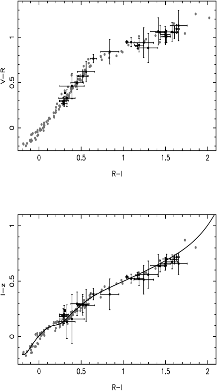
To check the accuracy of the photometric calibration, we considered the distribution in the (V-R,R-I) diagram of the stars present in the cluster field. The observed colours were corrected for the different seeing of the images as described in Sect. 5. In Fig. 3 (upper panel) we compare this distribution with that obtained from the synthetic stellar spectra of the HILIB library (Pickles PIC98 (1998)). The synthetic colours were produced by using the total efficiency curves of FORS2 and were calibrated with respect to the Vega spectrum. The observed and the synthetic distribution are in very good agreement, confirming the accuracy of data reduction and calibration, and the photometric quality of the observing nights.

Since no standard comparison fields were available for the z-band, we adopted the following calibration method. Synthetic z magnitudes were produced from the Pickles spectra and were calibrated by assuming ${\rm I-z=0}$ for the Vega spectrum. The zero point was obtained by fitting the distribution in the (R-I,I-z) diagram of the stars in the cluster field, corrected for seeing effects, to the locus of the synthetic colours. The result of the fit is illustrated in Fig. 3 (lower panel). The uncertainty on the zero point was estimated with the bootstrap method by taking into account the uncertainties on the colours of the stars. We obtained ${\rm ZP_{z}=25.216\pm 0.012}$. For the atmospheric extinction coefficient in the z-band, we assumed ${\rm A_{z}=0.08\leavevmode\nobreak\ mag/airmass}$, that is typical for the Paranal site.

Table 2: Results of the photometric calibration of the VRI data. Col. 1: waveband. Col. 2: colour C used in Eq. (1). Cols. 3, 4: colour term coefficients $\gamma$ and $\gamma^{\prime}$. Cols. 5, 6: atmospheric extinction coefficients ${\rm A}$ and ${\rm A^{\prime}}$. Cols. 7, 8: zero points ZP and ${\rm ZP^{\prime}}$ scaled to ${\rm 1sec}$. Col. 9: r.m.s. of the fitting residuals. The quantities marked by a prime are the FORS2 standard calibrations (see note 2). The uncertainties refer to $1\sigma$ standard intervals. Dots denote the quantities kept fixed in the fits (see text).

$$\begin{array}[]{ccccccccc}\vskip 3.0pt plus 1.0pt minus 1.0pt\cr\hline\cr&{\rm C}&{\rm\gamma}&{\rm\gamma^{\prime}}&{\rm A}&{\rm A^{\prime}}&{\rm ZP}&{\rm ZP^{\prime}}&{\rm\sigma}\\ \vskip 3.0pt plus 1.0pt minus 1.0pt\cr\hline\cr\vskip 3.0pt plus 1.0pt minus 1.0pt\cr{\rm V}&{\rm V-I}&{\rm.....}&{\rm 0.010\pm 0.005}&{\rm 0.18\pm 0.02}&{\rm 0.154\pm 0.007}&{27.280\pm 0.030}&{\rm 27.287\pm 0.014}&0.005\\ {\rm R}&{\rm V-R}&{\rm.....}&{\rm-0.018\pm 0.011}&{\rm 0.10\pm 0.01}&{\rm 0.114\pm 0.007}&{27.420\pm 0.013}&{\rm 27.450\pm 0.015}&0.013\\ {\rm I}&{\rm V-I}&{\rm-0.058\pm 0.004}&{\rm-0.059\pm 0.005}&{\rm.....}&{\rm 0.053\pm 0.007}&{26.474\pm 0.003}&{\rm 26.484\pm 0.037}&0.018\\ \vskip 3.0pt plus 1.0pt minus 1.0pt\cr\hline\cr\end{array}$$

4 K-band data

4.1 Reduction

The data reduction was performed by using ISAAC pipeline recipes included in Eclipse, version 4.0, the InfraRed Data Reduction (IRDR) software (see Sabbey et al. SML01 (2001)) and Fortran routines developed by the authors.

For both observing nights, we derived a dark frame by using the dark recipe of Eclipse. Since the dark variations between the two nights were less than $1-2\%$, the dark frames were averaged and then subtracted from all images. As shown in Fig. 4, a double ramp pattern along the column direction was noticeable in the scientific images after dark subtraction. The effect was found to be almost constant along the chip rows, varying from $\sim-5\%$ at the rows where the detector starts to be read out (rows 1 and 513), to $\sim 3-5\%$ at the rows read last. Since this pattern was not present in the flat-field frame, it must be a residual additive signal uncorrected by the dark subtraction. As discussed in the ISAAC Data Reduction Manual (version 1.5, Amico et al. ACD02 (2002)), this effect can be due to the dependece of the ISAAC infrared detector bias on time and on illumination flux. To remove such an effect, we applied a suitable correction immediately after dark subtraction. Each image was collapsed by taking the median along the row direction, and a low-pass filter was applied to the first 512 and to the last 512 samples of this signal in order to remove high frequency variations due to the noise and to the pixel to pixel response of the chip. The one-dimensional frame obtained by this procedure (see Fig. 4) was subtracted column by column from the original image, removing the ramp pattern at better than $\sim 1\%$.

Figure 4: Pattern remaining in the K-band images after dark subtraction. The gray line represents the signal after low-pass filtering (see text).

For the flat-field correction, we divided the scientific images by a differential flat-field frame, obtained by two sets of twilight sky exposures taken in the morning and in the evening, respectively. Each twilight exposure was corrected for the odd-even effect, particularly noticeable in the lower left quadrant (where it amounted to $\sim 2\%$ peak to peak variation). To this aim, we used the oddeven recipe of Eclipse. For each set of twilight images, a flat-field frame was obtained by subtracting high and low counts exposures in order to correct for residual additive components not removed by the dark subtraction. The final flat-field was derived by averaging the morning and evening twilight flats. This procedure allows to minimize intensity variation within the array at twilight. To test the accuracy of the flat-field correction, we compared the magnitudes of each photometric standard star at the different chip positions. The differences were found to be $\sim 5-7\%$ ($1\sigma$ standard level). To achieve higher accuracy, we applied an illumination correction by retrieving from the ESO archive the illumination frames closest in time to the date of our observations. After illumination correction, the variation were found to be $\sim 1\%$, that we assumed as the final accuracy of the flat-field.

The subsequent reduction included sky subtraction and image combining, that were performed by a two-step procedure. First, the images were processed by using the IRDR software. For each frame, a sky image was obtained by a robust mean of the eight nearest sequence exposures. After sky subtraction, a mask image was created for each frame by running SExtractor (Bertin & Arnouts 1996) with the checkimage OBJECTS option and was used to measure the dithering offsets. The first step coadded images were then obtained by combining the exposures within each sequence. At the second step, we created an object mask for the coadded images obtained at the first iteration by using SExtractor. These masks were expanded by a factor of 1.5 and de-registered to the corresponding dither exposures. Pixels with low and high counts in the flat-field were also included into the masks in order to reject hot and cold pixels. For each frame, the sky image was obtained by the average of the six nearest exposures rejecting masked pixels. The images were then coadded by using the IRAF task IMCOMBINE with a SIGCLIP algorithm for cosmic ray rejection.

4.2 Photometric calibration

The photometric calibration of the ISAAC data was performed by using standard stars from the list of Infrared NICMOS Standard Stars (Persson et al. PMK98 (1998)) and from the list of UKIRT standard stars (see Hunt et al. HMT98 (1998)).

The images were airmass-corrected by assuming an extinction coefficient ${\rm A_{K}=0.08\leavevmode\nobreak\ mag/airmass}$, typical for the period of our observations, and the total fluxes of the standard stars were estimated within a circular aperture of diameter $8^{\prime\prime}$. A small systematic difference of $\sim 0.05\leavevmode\nobreak\ {\rm mag}$ was found between the zero points derived from the UKIRT and NICMOS standard stars. Such result is not unexpected, since the UKIRT standards can be affected by small systematic and/or random errors with respect to those of the NICMOS list (see Sect. 5.2 of Persson et al. PMK98 (1998)). The final zero point was obtained, therefore, by considering only the NICMOS standard stars, and was estimated to be $24.34\pm 0.01\leavevmode\nobreak\ {\rm mag}$ (scaled to $1{\rm sec}$ exposure time). This is in good agreement with the value of the ISAAC pipeline (${\rm ZP\sim 24.36}$), relative to the period of our observations.

5 Aperture photometry

A catalogue of each image was produced by using the software SExtractor (Bertin & Arnouts BeA96 (1996)). Since the images have different seeing, particular care was taken in the choice of deblending parameters in order that objects were deblended in the same way for each band. For each object, we obtained magnitudes within a fixed aperture of diameter $2.3^{\prime\prime}$, corresponding to a physical size of ${\rm\sim 15\leavevmode\nobreak\ kpc}$ at ${\rm z=0.64}$, and magnitudes within an aperture of diameter ${\rm\alpha\cdot r_{K}}$, where ${\rm r_{K}}$ is the Kron radius (Kron KRO80 (1980)). We chose $\alpha=2.0$, for which the Kron magnitude is expected to enclose $92\%$ of the total flux. The total magnitudes were computed by adding $\mathrm{0.08\leavevmode\nobreak\ mag}$ to the Kron magnitudes.

Figure 5: Comparison of I-band high resolution and standard resolution aperture magnitudes. Differences are in the sense SR - HR. The dot – dashed line marks the aperture correction estimated by the method described in the text.

The catalogues were cross-correlated by deriving the coordinate transformation between each image and the V-band image. To this aim, we proceeded as follows. A first list of matched objects was obtained by using the IRAF task XYXYMATCH, with the triangle pattern algorithm. This method has the advantage to be robust with respect to geometric distortion effects in the images. The final transformations were obtained by fitting the coordinates of the objects in the matching list with polynomials of order 5, which allowed to correct for geometric distortion effects with an accuracy better than 0.5 pixel. The derived coordinate transformations were used to match the catalogues by using a nearest algorithm, producing a final list of ${\rm N=4868}$ sources detected in at least one band. For the objects with multiple K-band observations, the magnitudes turned out to be fully consistent within the photometric errors, and the final magnitudes were estimated by a weighted mean of the various measurements.

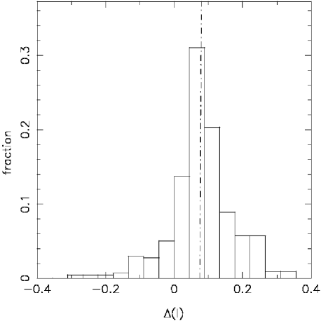
Since the images have different seeing (cfr. Table 1), the derivation of the colour indices requires suitable aperture corrections. To this aim, each image was convolved with a double gaussian kernel, whose parameters were chosen interactively to match the PSF of the image with the worst seeing (R band). Noise was added in order to compensate for the smoothing introduced by the convolution. The aperture corrections were estimated by the robust mean of the differences between the magnitudes of the objects in the original and the convolved images, and amount to $\mathrm{0.05\leavevmode\nobreak\ mag}$ in V, $\mathrm{0.03\leavevmode\nobreak\ mag}$ in I, $\mathrm{0.06\leavevmode\nobreak\ mag}$ in z, and $\mathrm{0.10\leavevmode\nobreak\ mag}$ in K. The corresponding uncertainties were estimated by the errors on the mean, and are $\mathrm{0.007\leavevmode\nobreak\ mag}$, $\mathrm{0.013\leavevmode\nobreak\ mag}$, $\mathrm{0.02\leavevmode\nobreak\ mag}$, and $\mathrm{0.03\leavevmode\nobreak\ mag}$ in V, I, z and K, respectively. These values were added in quadrature to the photometric errors of the magnitudes. To test our procedure, we compared the magnitudes of the sources in common between the standard and high resolution I-band images, whose seeing values are $0.3^{\prime\prime}$ and $0.8^{\prime\prime}$, respectively. The magnitude differences are shown in Fig. 5 together with the aperture correction derived as described above. The figure demonstrates the accuracy of the adopted method.

The completeness in each band was estimated following the method of Garilli et al. (GAR99 (1999)), that consists in the determination of the magnitude at which the objects start to be lost since they are below the brightness threshold in the detection cell. Details will be given elsewhere (Massarotti et al. 2002, in preparation). The completeness magnitudes in V-, R-, I-, z- and K-band are 25.7, 25.0, 23.2, 22.5 and 21.2 respectively.

6 Photometric redshifts

Photometric redshifts were estimated according to the Spectral Energy Distribution (SED) fitting method (see Massarotti et al. 2001a, b, and references therein). In order to achieve a reasonable accuracy, we considered galaxies with signal-to-noise ratio $\mathrm{S/N>5}$ in at least three bands. This sample contains ${\rm N=633}$ galaxies, of which ${\rm N=360}$ have K-band information, and is complete up to the total magnitude ${\rm I_{T}=22.5}$.

Figure 6: Distribution of photometric redshifts $z_{\mathrm{p}}$ for galaxies with $18.5\leq I\leq 22.5$, after subtraction of the field counts estimated by the VIRMOS survey data. The dashed line marks the redshift 0.64.

The photometric redshifts were derived as described in Busarello et al. (BML02 (2002)), here we briefly outline the technique. Taking into account the depth of our imaging, we looked for redshifts in the range $z\in[0.0,2.5]$ with a step of 0.01. Model galaxy spectra were provided by the code of Bruzual & Charlot (BrC93 (1993)). The adopted templates consist of models with a Scalo (SCA86 (1986)) IMF and with an exponential SFR $e^{-t/\tau}$. We chose $\tau=1,4,15$ Gyr, to describe the colours of $E/S0$, $Sa/Sb$, and $Sc/Sd$ templates. To allow for different metallicities of early-type galaxies, we introduced $E/S0$ models with ${\rm Z/Z_{\odot}}=$0.2, 0.4, 1 and 2.5, while template spectra evolution was followed in the time interval $t\in[0.01,12.0]$ Gyr. To estimate the uncertainty ${\rm\Delta z_{p}}$ in the photometric redshift, we performed numerical simulations by taking into account the uncertainties on magnitudes. Since the K-band does not cover the whole cluster field, we investigated the possible bias on $\mathrm{z_{p}}$ for the galaxies without K-band data. To this aim, we compared the photometric redshifts obtained for the sources with $\mathrm{I_{T}<22.5}$ (a) by taking into account and (b) by ignoring the K-band. The number of galaxies which were found to be cluster members in case (a) and no cluster members in case (b), and viceversa, turned out to be negligible ($<5\%$).

We defined a galaxy as a cluster member when the photometric redshift is in the range ${\rm z_{p}\in[0.54,0.74]}$. However, to obtain a reliable sample of cluster members via photometric redshifts it is crucial to take into account possible degeneracies of template colours at different redshifts. By inspecting colours of GISSEL98 templates, we found that some degeneracy exists between colours of blue $Sc/Sd$ galaxies at the cluster redshift ($\mathrm{V-R=0.94}$, $\mathrm{R-I=0.94}$, $\mathrm{I-K=2.62}$ with $\mathrm{t_{form}=12\leavevmode\nobreak\ Gyr}$, $Z=Z_{\odot}$) and those of red $E/S0$ galaxies at $z\sim 0.3$ ($\mathrm{V-R=1.04}$, $\mathrm{R-I=0.82}$, $\mathrm{I-K=2.80}$ with $\mathrm{t_{form}=12\leavevmode\nobreak\ Gyr}$, $Z=Z_{\odot}$). To correct for this effect, we also considered as cluster members the objects having $z\in[0.3,0.4]$ and ${\rm\Delta z_{p}}$ consistent with the cluster redshift. We found that ${\rm N=19}$ galaxies satisfy this criterion. Most of these galaxies ($\sim 75\%$) turn out to be disk dominated objects and therefore their late spectral type is also supported by the shape of the light profile (Sect. 7). The final list of cluster members brighter than ${\rm I=22.5}$ consists in ${\rm N=171}$ galaxies.

To gain insight into the contamination by field galaxies in our sample, we used the VIRMOS preparatory photometric survey as the control sample. These data, kindly provided by the VIRMOS Consortium (Le Fèvre et al. 2002, in preparation), are actually the proper dataset for estimating the field contamination in our sample because of their large field, similar filters and high depth). In particular, to estimate the redshift distribution for field galaxies we used the VIRMOS catalogues (VRIK, McCracken et al. 2002, in preparation) relative to a 150 arcmin² field with available K-band photometry. It has to be noticed that the photometric redshifts were obtained for the field and the cluster by using a similar photometric baseline and the same procedure. The distribution of photometric redshifts, after subtraction of the field counts, is shown in Fig. 6 for the objects with $18.5\leq$ I $\leq 22.5$, corresponding to the magnitude range of cluster galaxies up to the completeness limit of the sample with photometric redshifts. It is dominated by the peak around the cluster redshift. The FWHM of the peak is $\sim 0.1$ and is due to the intrinsic redshift distribution of the cluster members and to the errors on photometric redshifts. The redshift distribution of VIRMOS galaxies is in full agreement with that relative to the cluster field outside of the peak at $\mathrm{z}\sim 0.64$, thus confirming the effectiveness of our selection procedure and the reliability of the VIRMOS control field. In the field of EIS 0048 we found $\mathrm{N}=140\pm 12$ galaxies with $\mathrm{z}<0.5$ and $\mathrm{N}=46\pm 7$ galaxies with $0.8<\mathrm{z}<1.8$, while in the same redshift ranges the number of galaxies predicted on the basis of the control sample are $\mathrm{N}=141.5\pm 6.6$ and $\mathrm{N}=43\pm 4$ respectively. According to the VIRMOS data, $\mathrm{N}=48\pm 4$ ($25\%$) galaxies of the cluster sample are expected to be field galaxies.

In Fig. 7 we compare photometric ($z_{\mathrm{p}}$) and spectroscopic ($z_{\mathrm{s}}$) redshifts for a sub–sample of 25 cluster galaxies (Busarello et al. 2002, in preparation, and C. Lobo, private communication). We notice that all the spectroscopically confirmed cluster members satisfy the selection criterion previously discussed.

Figure 7: Comparison of spectroscopic $z_{\mathrm{s}}$ and photometric redshifts $\mathrm{z_{p}}$ for 25 spectroscopically confirmed cluster members.

7 Galaxy shape classification

Although a proper morphological classification requires the high quality of the HST images, relevant information on the properties of the light distribution of distant galaxies can be obtained by using ground based data (see La Barbera et al. LBM02 (2002), hereafter LBM02, and references therein). We used the procedure described in LBM02 to model the surface brightness distribution of galaxies in the cluster field, by fitting Sersic models convolved with the PSF of our images. This analysis will be presented in detail in a forthcoming paper.

For the present work, we will use the information on the shape of the galaxy light profiles as parametrized by the Sersic index n. We fitted Sersic models both to the standard resolution (SR) and to the high resolution (HR) I-band images. Accurate structural parameters for the galaxies at the redshift of EIS 0048 can be obtained from the very good seeing of the HR images (La Barbera et al. 2002, in preparation). Nevertheless, we found that a reliable separation between galaxies with low n value (disks) and galaxies with a higher value of the shape parameter (spheroids) can be also done with our SR images, allowing us to perform the galaxy shape classification in the whole observed field. In fact, only $\sim 8\%$ of the galaxies brighter than ${\rm I_{T}=22}$ have a different classification in the HR and the SR images, while the number of mismatches increases to $\sim 17\%$ at ${\rm I_{T}\sim 22.5}$. Moreover, for the galaxies with discordant classification we did not find any significant systematic effect: $\sim 10\%$ of the galaxies defined as disks on the basis of the HR data are classified as spheroids in SR, and vice-versa for the remaining $\sim 7\%$.

We chose ${\rm n=2}$ to discriminate between the two classes of galaxies. As shown by numerical simulations (see van Dokkum et al. vDF98 (1998)), this criterion corresponds to separate objects with a low bulge fraction ($<20\%$) from galaxies with a larger bulge component. Our final sample of galaxies with shape information consists of all the ${\rm N=171}$ cluster members brighter than ${\rm I_{T}=22.5}$.

8 Colour-magnitude relations

The optical (V-I) and NIR (V-K) colour-magnitude diagrams for the objects in the cluster field are shown in Fig. 8. The black dots denote objects brighter than $\rm{I_{T}}=22.5$ defined as cluster members according to their photometric redshift (see Sect. 6), while different symbols are used to mark disks and spheroids. At this magnitude limit, we have shape classification for all the cluster members.

Figure 8: Colour-magnitude diagrams for the galaxies in the cluster field (gray circles). Black symbols denote objects with $\rm{I_{T}}<22.5$ defined as cluster members on the basis of their photometric redshift. Circles denote the spheroids, while disks are marked by crosses. The dashed lines are the best fits to the CM while the dotted lines limit the $\pm\sigma$ intervals. The error bars in the left corners of the plots indicate the mean uncertainties on colours and magnitudes at $\mathrm{I_{T}\sim 19.7}$ and $\mathrm{I_{T}\sim 22.2}$ for the upper plot and at $\mathrm{K_{T}\sim 17}$ and $\mathrm{K_{T}\sim 19}$ for the lower plot.

8.1 Distribution in the CM planes

Spheroids define sharp CM relations both in the (V-K,K) and in the (V-I,I) planes. The sequences extend for at least 3 magnitudes, up to the completeness limits of our samples, and are defined in the plots by the loci enclosed within the dotted lines (see next section for details). It is interesting to notice that 43 spheroids are significantly bluer with respect to the $V-I$ red sequence, among them 24 are bluer in the range $[-0.4,-0.2]\leavevmode\nobreak\ \mathrm{mag}$. In particular, we find six blue spheroids at very bright magnitudes ($\mathrm{I_{T}}<20.2$ and ${\rm 1.9<V-I<2.2}$). Two of these have also K-band photometry and lie on the red locus in the (V-K,K) plane. We verified that the classification of these blue spheroids is the same in all our images, and therefore it is not affected by a possible uncertainty on the Sersic index. Most of the disks (43) are bluer with respect to the optical red locus, although $10$ galaxies do not show significant deviations and other two have redder colours. Four of these 12 galaxies have K-band photometry and are located above the V-K CM relation.

Since our sample is selected by the photometric redshift technique, some considerations are needed about the contamination by field objects in our diagrams. On the VIRMOS data, in the (V-I,I) plane we expect $39.5\pm 3.5$ blue galaxies, $8\pm 1.6$ red sequence objects and $0.6\pm 0.4$ redder galaxies. These numbers indicate that the presence of blue spheroids and red disks is not due to the field contamination but that at least some of these objects are real cluster members. Moreover, on the basis of the comparison field sample, the cluster membership of the bright blue spheroids is highly significant. In fact, in the range of magnitude and colours of these galaxies, we expect that only $0.5\pm 0.5$ objects could be field contaminants.

8.2 Slope and zeropoint of the CM relations

We study the CM relation of EIS 0048 by comparing our results with the models of KABA98. We performed a linear regression of the V-K and V-I colour-magnitude sequences by considering the following relations:

$${\rm V-I\,} = {\rm A_{VI}+B_{VI}\cdot I}$$ (2)

$${\rm V-K} = {\rm A_{VK}+B_{VK}\cdot K}.$$ (3)

The fits were done by minimizing the bi-weight scatter of the residuals (see Beers, Flynn & Gebhardt BFG90 (1990)), and the algorithm was modified in order to weight each point with the corresponding uncertainty on the photometric redshift estimate. Only objects within the completeness limit of our photometry were considered. This procedure allows to minimize the effect of outliers and of objects with poor photometric information and/or cluster membership. We also verified that the fitting results do not change by excluding disks from our sample. The uncertainties on the fitting parameters were obtained by numerical simulations of the distributions in the CM planes. For the optical relation, we obtained ${\rm A_{VI}=3.95\pm 0.30\leavevmode\nobreak\ mag}$ and ${\rm B_{VI}=-0.073\pm 0.015}$, with a r.m.s. of the residuals that amounts to ${\rm\sigma_{VI}=0.10\pm 0.03\leavevmode\nobreak\ mag}$. For the NIR, due to the smaller sample size, the relative uncertainty on the CM slope is large: ${\rm B_{VK}=-0.15\pm 0.08}$. Therefore, we chose to repeat the fit by using a fixed value of the slope ${\rm B_{VK}=-0.11}$, that is typical for the spheroids in clusters at the same redshift (see Fig. 4 in KABA98). This gives ${\rm A_{VK}=7.75\pm 0.05\leavevmode\nobreak\ mag}$, with r.m.s. of the residuals ${\rm\sigma_{VK}=0.14\pm 0.06\leavevmode\nobreak\ mag}$. The fits to the CM relation are shown in Fig. 8 along with the relative $3\leavevmode\nobreak\ \sigma$ intervals. We denote an object as a blue galaxy if it lies more than $3\leavevmode\nobreak\ \sigma$ below the (V-I,I) CM fit, as a red galaxy otherwise.

Figure 9: I-band image of the cluster field. The map of the counts density is represented by the gray contours. The grey intensity is proportional to the density value. Triangles and circles mark disks and spheroids respectively.

By considering the previous results, we see that the dispersions around the optical and NIR CM relations can be fully explained by the typical uncertainty on galaxy colours (${\rm\sim 0.1\leavevmode\nobreak\ mag}$, cfr. Fig. 8), and that, therefore, the intrinsic scatter of the relations is very small. Unfortunately, due to the field contamination and to the uncertainty on morphological selection, the quoted errors on the dispersions are too large to obtain an accurate quantitative estimate of the intrinsic scatter. The fitting coefficients of the Eqs. (3) can be compared with the predictions of the KABA98 models relative to the ${\rm V_{555}-I_{814}}$ vs. ${\rm I^{T}_{814}}$ and the ${\rm V-K}$ vs ${\rm K^{T}}$ CM relations considered by the authors (see Figs. 4, 5 in KABA98), where ${\rm V_{555}}$ and ${\rm I_{814}}$ are the magnitudes of the HST filters. By comparing the value of ${\rm B_{VI}}$ with the values shown in Fig. 4 (right middle panel) in KABA98, we see that our estimate is fully consistent with the prediction of a pure metallicity sequence with an old epoch (${\rm z_{f}=4.5}$) of galaxy formation. Pure metallicity models, with a more recent formation epoch, ${\rm z_{f}=1.7}$ and ${\rm z_{f}=1.2}$, are discarded at $1.5\sigma$ and $2.0\sigma$ confidence level respectively. The zero points of the CM relations can be compared with the values shown in Fig. 5 in KABA98. To this aim, we referred the ${\rm A_{VI}}$ and ${\rm A_{VK}}$ coefficients to the magnitudes $\mathrm{K_{T}}=-25.5$ and $\mathrm{I_{T}}=-22$, by using the same cosmology adopted by KABA98 (${\rm H_{0}=50\leavevmode\nobreak\ Km\leavevmode\nobreak\ s^{-1}Mpc^{-1}}$, $\Omega_{m}=0.3$, $\Omega_{\Lambda}=0.7$) and by estimating ${\rm K}$ corrections from Poggianti (Pog97 (1997)). For the NIR, we obtain a corrected value of the zero point ${\rm A^{c}_{VK}=5.58\pm 0.05\leavevmode\nobreak\ mag}$, that is consistent with the models of KABA98 having ${\rm z_{f}\geq 1.7}$, while younger models are not consistent with our data. For the optical zero point, we obtain ${\rm A^{c}_{VI}=2.33\pm 0.03\leavevmode\nobreak\ mag}$ that is about 0.2 mag below the value relative to the model with ${\rm z_{f}\sim 4.5}$. We notice, however, that this difference can be affected by the uncertainty on the zero point of the HST photometry (see e.g. Holtzman et al. HBC95 (1995)), making this disagreement not significant. In fact, the comparison of the ${\rm R-K}$ CM with KABA98 gives the same results obtained for the ${\rm V-K}$ relation. Moreover, we notice that the ${\rm V-I}$ colour predicted by the GISSEL98 synthesis code (see Bruzual & Charlot BrC93 (1993)) for an E template, with solar metallicity and with ${\rm z_{f}}=4.5$, is ${\rm 2.34\leavevmode\nobreak\ mag}$, in full agreement with the value of ${\rm A^{c}_{VI}}$.

9 Spatial distribution of cluster populations

To further investigate the properties of the blue and red galaxy populations, we analyzed their spatial distribution in the cluster field. In Fig. 9, we show a map of the number density of the objects defined as cluster members according to their photometric redshifts. Cluster galaxies show an evident clumpy distribution: the peak of the density is associated to a main structure having projected radius $\sim 1.0^{\prime}-1.5^{\prime}$ ($\mathrm{\sim 0.5\leavevmode\nobreak\ Mpc}$ at ${\rm z=0.64}$), while at least two secondary clumps of galaxies are found at a distance of $\sim 3.0^{\prime}$ ($\mathrm{\sim 1.2\leavevmode\nobreak\ Mpc}$) from the main peak. Although we cannot quantify the number of spheroid and disks that are expected to be field objects, it is quite remarkable that the various structures are populated, mostly, by galaxies with a more concentrated shape, while disks are found preferably in the low density regions.

Figure 10: Map of the counts density for the red and blue cluster populations (upper and lower panels). The grey scale is the same for both panels.

By using the separation between red and blue galaxies discussed in Sect. 8.2, we constructed the density maps relative to the two classes of objects (see Fig. 10). The clumps of galaxies defining the cluster structure are evident in the plot relative to the red population, for which we expect a very low field contamination ($\sim 7\%$). With the exception of a possible clump near the border of the field, the density map of the blue population does not show any particular structure. This is partly due to the field contamination, but it could also indicate that cluster blue galaxies do not share the same spatial distribution of the red ones. In fact, if we construct the density map of the blue galaxies, by weighing each object with the relative luminosity, we find that the clumps present in the lower panel of Fig. 10 outside the region corresponding to the cluster central structure, become the dominant features in the plot. We point out, however, that a spectroscopic survey in the field is needed in order to definitely exclude the contamination effect.

10 Butcher-Oemler effect

In order to derive the fraction of blue galaxies ${\rm f_{B}}$ in the cluster EIS 0048, we followed the procedure of Butcher & Oemler (1978a , 1978b ). We computed the fraction of galaxies that are ${\rm 0.2\leavevmode\nobreak\ mag}$ bluer than the red sequence in the rest-frame (B-V,V) diagram within a magnitude limit ${M_{V}=-20}$, and that are enclosed within ${R_{30}}$, the radius containing $30\%$ of the total galaxy population.

Figure 11: Density profile of the galaxies defined as cluster members. Error bars denote Poissonian uncertainties. Density have been arbitrarily scaled in order to have a density of $\mathrm{1\leavevmode\nobreak\ gal/arcmin^{2}}$ for the field (dashed horizontal line). The curves show the models fitted to the density profile (see upper-right).

In Fig. 11, we show the density profile of the cluster members derived by considering circular coronae centered on the peak of the density map (see Fig. 9) with the suitable correction for the rectangular geometry of our field. The density counts relative to the cluster core decrease gradually up to a distance of ${\rm\sim 2\leavevmode\nobreak\ arcmin}$, while the substructures of Fig. 9 are shown by the increase of the profile between ${\rm R=2^{\prime}}$ and ${\rm R=4^{\prime}}$. At large distances, the density is very close to the value expected in the field, showing that the estimate of field contamination is reliable. To derive the value of ${\rm R_{30}}$, we need to predict the fraction of cluster galaxies ${\rm f_{O}}$ expected out of the observing field. To this aim, we used an extrapolation of the density profile, by fitting the density counts of the cluster core (${\rm R<2^{\prime}}$) by different models. We considered the models adopted by Adami et al. (AMK98 (1998)) to analyze a large sample of nearby clusters: the generalized Hubble and King profiles, the generalized NFW (see Navarro, Frenk & White NFW95 (1995), NFW96 (1996)) and de Vaucouleurs models. The fitted profiles were integrated from ${\rm R=4^{\prime}}$ up to an Abell radius (${\rm 3h_{50}^{-1}Mpc}$), giving ${\rm f_{O}=20\pm 5\%}$. This value was used to calculate ${\rm R_{30}}$ and the concentration parameter ${\rm C=\log(R_{60}/R_{20})}$, where ${\rm R_{p}}$ is the radius that encloses ${\rm p\%}$ of the total number of cluster galaxies. The same procedure was repeated by extrapolating the density profile out of ${\rm R}=2^{\prime}$, without considering the substructures present between ${\rm R}=2^{\prime}$ and ${\rm R}=4^{\prime}$. In Table 3 we report the values of ${\rm C}$ and ${\rm R_{30}}$ estimated for case 1 (R$<2^{\prime}$) and for case 2 t(R$<4^{\prime}$), and the corresponding uncertainties, obtained by taking into account the Poissonian error on our number counts and the uncertainty on the density of field counts. As it was expected, the value of ${\rm R_{30}}$ is smaller for case 1, and ranges between ${\rm R_{30}}\sim 1^{\prime}$ and ${\rm R_{30}}\sim 1.5^{\prime}$, while the value of ${\rm C}$ varies from $\sim 0.43$, that is typical of a not particurarly compact cluster, to $\sim 0.5$, that is closer to that of a more rich, concentrated structure (see Butcher & Oemler 1978b ). To check our estimate of ${\rm R_{30}}$ and ${\rm C}$, we repeated the calculation by considering only the red cluster members. We obtained ${\rm R_{30}}=1.2\pm 0.1$ and ${\rm C}=0.53\pm 0.02$ for case 1, while ${\rm R_{30}}=1.5\pm 0.19$ and ${\rm C}=0.44\pm 0.013$ for case 2. These values are fully consistent with those reported in Table 3.

Table 3: Standard parameters for the computation of the BO effect. See text for details.

$$\begin{array}[]{lcccc}\vskip 3.0pt plus 1.0pt minus 1.0pt\cr\hline\cr&{\rm C}&{\rm\Delta C}&{\rm R_{30}}&{\rm\Delta R_{30}}\\ &&&(^{\prime})&(^{\prime})\\ \hline\cr{\rm 1(R<2^{\prime})}&0.50&0.02&1.0&0.07\\ {\rm 2(R<4^{\prime})}&0.43&0.02&1.5&0.17\\ \hline\cr\end{array}$$

The blue fraction ${\rm f_{B}}$ was computed by using the ${\rm V-I}$ colour index, that is very close to ${\rm B-V}$ rest-frame at the cluster redshift. In order to convert ${\rm V-I}$ colour into ${\rm B-V}$ rest-frame, we used the synthesis code of Bruzual & Charlot (1993) to construct galaxy templates with different age, metallicity, star formation rate, and dust content, and we computed for each of them ${\rm V-I}$ and ${\rm B_{r}-V_{r}}$ colours, where $\mathrm{B_{r}}$ and $\mathrm{V_{r}}$ are magnitudes in the redshifted B and V filters. The relation between the two colours was found to be described very well by a polynomial of degree four, with a very small r.m.s. of $0.025{\rm\leavevmode\nobreak\ mag}$. The same procedure was adopted to convert the ${\rm I}$ magnitudes into rest-frame V-band magnitudes. The value of ${\rm f_{B}}$ was computed by subtracting the fraction of blue galaxies obtained for the cluster sample to that expected for the field. The calculation was performed by considering only galaxies brighter than ${\rm M_{V}}=-20$, that corresponds to ${\rm I}\sim 22.5$ at ${\rm z=0.64}$. We notice that this corresponds to the completeness limit of our cluster sample. The uncertainty on ${\rm f_{B}}$ was estimated by taking into account Poissonian and photometric errors of both cluster and field samples. In Fig. 12, we show the trend of ${\rm f_{B}}$ versus the cluster-centric distance. At distances between ${\rm R=1^{\prime}}$ and ${\rm R=1.5^{\prime}}$, that enclose our estimate of ${\rm R_{30}}$ (cfr. Table 3), we obtain ${\rm f_{B}=0.11\pm 0.07}$. We notice that this result is very robust with respect to our computation of ${\rm R_{30}}$: ${\rm f_{B}}$ is, in fact, practically constant between ${\rm R}=1^{\prime}$ and ${\rm R=}2^{\prime}$.

Figure 12: Fraction of blue galaxies within R, where R is the cluster-centric distance.

The blue galaxy fraction of the cluster EIS 0048 can be compared with the value predicted by the standard BO effect at ${\rm z=0.5}$, ${\rm f_{B}=0.25}$, and the values obtained by recent works, who have attempted to compute the BO effect at ${\rm z>0.5}$. In particular, the BO effect has been investigated at ${\rm z\sim 0.8}$ by van Dokkum et al. (vDF00 (2000)), who found ${\rm f_{B}=0.22\pm 0.05}$, and by Rakos & Schombert (RaS95 (1995)), who estimated a very high blue galaxy fraction, ${\rm f_{B}\sim 0.8}$. In agreement with van Dokkum et al. (vDF00 (2000)), our results do not indicate a high increase in the BO effect at ${\rm z>0.5}$. The cluster EIS 0048 at ${\rm z=0.64}$ shows a quite low blue galaxy fraction, about one half of the standard BO effect at ${\rm z=0.5}$. By looking at Fig. 12, it is also interesting to notice that the value of ${\rm f_{B}}$ seems to increase at distances greater than ${\rm R=2^{\prime}}$ up to $\sim 23\%$ at ${\rm R=4^{\prime}}$. This would be consistent with what found by previous studies at lower redshift (e.g. Kodama & Bower KOB01 (2001), Fairley et al. FJW02 (2002)), and can be explained as a consequence of accretion of field galaxies into the cluster structure.

11 Summary.

We have studied the properties of the galaxy populations in the cluster $\mathrm{EIS\,0048}$   at $z=0.64$, by using a large photometric baseline including V-, R- I-, z- and K-band data. Cluster members have been selected by using the photometric redshift technique, producing a final list of $\mathrm{N=171}$ galaxies complete up to $\mathrm{I=22.5}$. To estimate the field contamination, we used as control sample the VIRMOS preparatory photometric survey, for which photometric redshifts were estimated by using the same procedure adopted for the cluster sample. Out of the $\mathrm{N=171}$ candidate members, N=48 objects are expected to be field contaminants. Cluster galaxies have been classified into disks and spheroids on the basis of the shape of the light profile parametrized by the Sersic index $\mathrm{n}$. The contamination between the two classes is expected to vary from $\sim 8\%$ at $\mathrm{I=22}$ to $\sim 17\%$ at $\mathrm{I=22.5}$.

Colour – magnitude distributions.

Spheroids and disks show an evident segregation in the CM diagrams. The first family of galaxies define a sharp red sequence both in the optical and in the NIR, while disks have in general bluer colours and are located preferably below the CM relations. We find, however, some level of mixing between the properties of the two classes: some spheroids have blue colours, while some disks are red or redder than the red sequences. Interestingly, some of the blue spheroids are found at bright magnitudes (I $<20$) and are not expected to be field contaminants.

Spatial distributions.

Disks and spheroids show a sharp spatial segregation, with disk galaxies found preferably in the low density regions. The spheroid population defines a central structure with a diameter of $\sim 1.0\leavevmode\nobreak\ Mpc$, and secondary clumps located at a distance $>1.0$ Mpc from the main density peak. By analyzing the density map of blue and red galaxies, we find that the two populations have a very different spatial distribution, the blue galaxies showing an amorphous structure.

A standard Butcher – Oemler analysis has been performed in order to derive the fraction of blue cluster galaxies. The cluster $\mathrm{EIS\,0048}$   is characterized by a concentration parameter $\mathrm{C\sim 0.45}$, that is intermediate between a very rich cluster and a less concentrated, poor structure. The radius that encloses $30\%$ of the total galaxy population is comprised between $1$ and $1.5$ arcmin ($0.4-0.6\leavevmode\nobreak\ \mathrm{Mpc}$). The fraction of blue galaxies amounts to $\mathrm{0.11\pm 0.07}$, and increases up to $\sim 23\%$ at a distance of $\sim 1.6\leavevmode\nobreak\ \mathrm{Mpc}$. We do not find, therefore, a strong BO effect in the cluster $\mathrm{EIS\,0048}$ at $\mathrm{z=0.64}$, in agreement with previous studies who did not find a high increase of the fraction of blue galaxies at $\mathrm{z>0.5}$.