Gravitational waves from stars orbiting the Sagittarius A^∗ black hole

Abstract

One of the main astrophysical processes leading to strong emission of gravitational waves to be detected by the future space-borne interferometer LISA is the capture of a compact star by a black hole with a mass of a few million solar masses in the center of a galaxy. In previous studies, main sequence stars were thought not to contribute because they suffer from early tidal disruption. Here we show that, according to our simulations of the stellar dynamics of the Sgr A^∗ cluster, there must be one to a few low-mass main sequence stars sufficiently bound to the central Galactic black hole to be conspicuous sources in LISA observations. The probability that a white dwarf may be detectable is lower than $0.5$ and, in spite of mass segregation, detection of a captured neutron star or stellar black hole in the center of the Milky Way is highly unlikely.

1 Introduction

Recently, the presence of massive black holes (MBHs, with masses from a few $10^{5}$ to a few $10^{9}M_{\odot}$) in the center of non-active galaxies has received considerable observation support, mainly from the kinematics of stars or gas in the center-most region of nearby galaxies (Kormendy & Gebhardt 2001). One of the most convincing cases is the Milky Way for which the motion of individual stars can be observed, both along the line of sight or perpendicular to it (Genzel et al. 2000; Ghez et al. 2000; Schödel et al. 2002). They orbit a dark mass of $2.6\times 10^{6}\,M_{\odot}$ whose extent is less than 0.001 pc and coincides with the radio source Sgr A^∗.

These MBHs reside at the center of stellar clusters whose densities may exceed $10^{7}\,M_{\odot}\,\mathrm{pc}^{-3}$ (Lauer et al. 1998; Alexander 1999). An exciting consequence of this is the possibility for a star to be captured onto a relativistic orbit around the MBH by emission of gravitational radiation (Hils & Bender 1995; Sigurdsson & Rees 1997; Freitag 2001; Ivanov 2002). For a source at a distance of a few hundreds of Mpc and a MBH’s mass in the range between $10^{4}$ and $10^{7}\,M_{\odot}$, the frequency of these waves will enter LISA’s range as the orbit shrinks down (Thorne 1998; Danzmann 2000). If it withstands the tidal forces, the star will eventually find itself on an unstable, plunging orbit and disappear through the BH’s horizon. The computation of the late, strong-field, phases of this inspiral requires full general relativistic treatment and cannot be handled with tools presently available (see Glampedakis & Kennefick 2002; Glampedakis et al. 2002 and references therein). Nevertheless when the pericenter distance, $R_{\mathrm{p}}$ is still well beyond the stability limit ($3R_{\mathrm{S}}=6GM_{\mathrm{BH}}c^{-2}$ for a circular orbit around a non-rotating BH, with $G$ the gravitational constant, $M_{\mathrm{BH}}$ the BH’s mass and $c$ the speed of light), approximate methods can be used to determine how the orbit evolves through emission of gravitational waves. For a star with mass $M_{\ast}$ on an initial orbit of semi-major axis $a_{0}$ and high eccentricity, $1-e_{0}\ll 1$, the time to plunge is approximately (Peters 1964)

$$T_{\mathrm{plunge}} \simeq \frac{2^{1/2}24}{85}\frac{c^{5}}{G^{3}M_{\mathrm{BH}}^{2}M_{\ast}}(1-e_{0})^{7/2}a_{0}^{4}\simeq 3.2\times 10^{6}\,\mathrm{yrs}$$

$$\times\left(\frac{M_{\mathrm{BH}}}{10^{6}\,M_{\odot}}\right)^{2}\left(\frac{M_{\ast}}{1\,M_{\odot}}\right)^{-1}\left(\frac{R_{\mathrm{p}}^{0}}{10\,R_{\mathrm{S}}}\right)^{4}\left(\frac{1-e_{0}}{10^{-5}}\right)^{-1/2},$$

where $R_{\mathrm{p}}^{0}$ is the initial pericenter distance. Compact stars, i.e. white dwarfs (WDs), neutron stars (NSs) or stellar black holes (SBHs) spiral all the way down to the horizon but a main sequence star (MSS) is torn apart by the tidal gravitational field of the MBH at a distance $R_{\mathrm{d}}=k(M_{\mathrm{BH}}/M_{\ast})^{1/3}R_{\ast}\simeq 50\,k\,R_{\mathrm{S}}(M_{\mathrm{BH}}/10^{6}\,M_{\odot})^{-2/3}(\bar{\rho}_{\ast}/1\,\mathrm{g}\,\mathrm{cm}^{-3})^{-1/3}$, where $R_{\ast}$ is the radius of the star, $\bar{\rho}_{\ast}$ its average density and $k$, a constant of order unity, depends on the stellar structure (Hills 1975; Rees 1988) . Hence a MSS may come close enough to the MBH to emit significant amounts of gravitation radiation only if it is compact enough. Note that $\bar{\rho}_{\ast}$ is maximum for $M_{\ast}\simeq 0.07\,M_{\odot}$, at the transition to brown dwarfs (Chabrier & Baraffe 2000).

We only consider quadrupolar gravitational radiation because it dominates energy and angular momentum losses. In the weak field approximation and neglecting the gravitational influence of other stars, the orbit may be treated as a Keplerian ellipse whose parameters slowly change as a result of emission of gravitational radiation. The latter is emitted at integer multiples of the orbital frequency, $\omega_{n}=n(GM_{\mathrm{BH}})^{1/2}a^{-3/2}$. At a distance $D$ from the source, the strain amplitude in the $n^{\mathrm{th}}$ harmonic is

$$h_{n} = \gamma(n,e)\frac{1}{D}\frac{G^{2}M_{\mathrm{BH}}M_{\ast}}{c^{4}a}$$

$$\simeq 2\times 10^{-27}\gamma\left(\frac{D}{1\,\mathrm{Mpc}}\right)^{-1}\left(\frac{a}{1\,\mathrm{pc}}\right)^{-1}\left(\frac{M_{\mathrm{BH}}}{10^{6}\,M_{\odot}}\right)\left(\frac{M_{\ast}}{1\,M_{\odot}}\right),$$

where the non-dimensional factor $\gamma$ is an intricate function of $n$ and the eccentricity $e$ (Peters & Mathews 1963; Pierro et al. 2001). For simplicity, we consider the the rms amplitude, averaged over $+$ and $\times$ polarizations and all directions.

We assume that a star is irremediably captured by the MBH if it gets on an orbit with a time scale for shrinkage by emission of gravitational radiation shorter than the time over which 2-body relaxation could significantly modify the pericenter distance, $T_{\mathrm{mod}}\simeq\theta^{2}T_{\mathrm{rel}}<T_{\mathrm{rel}}$ (Sigurdsson & Rees 1997; Ivanov 2002). $T_{\mathrm{rel}}$ is the usual relaxation time (Binney & Tremaine 1987) and $\theta$ is the angle between the trajectory and the direction to the center. The typical eccentricity of capture orbits may be estimated from the condition $T_{\mathrm{plunge}}<T_{\mathrm{rel}}$:

$$1-e<\left(\frac{V_{\mathrm{orb}}}{c}\right)^{\!\!10/7}\!\!\left(\frac{M_{\mathrm{BH}}}{M_{\mathrm{cusp}}}\right)^{\!\!2/7}\simeq 10^{-5}\left(\frac{V_{\mathrm{orb}}}{100\,\mathrm{km\,s}^{-1}}\right)^{\!\!10/7}.$$ (3)

Here, $V_{\mathrm{orb}}$ is a typical velocity for stars in the “cusp”, i.e. the central region of the cluster where the kinematics is dominated by the gravitational attraction of the MBH. $M_{\mathrm{cusp}}$, of order $M_{\mathrm{BH}}$, is the total stellar mass in this region. The rate of capture is controlled by processes that send stars onto these extremely elongated orbits. In a spherical cluster, the most important one is 2-body relaxation.

2 Numerical model of the central cluster

To compute capture rates, many difficulties have to be faced, in particular the role of mass segregation, stellar collisions or tidal disruptions. Although these complications can be included to some extent into analytical computations (Sigurdsson & Rees 1997; Miralda-Escudé & Gould 2000), the intricate nature of the problem calls for numerical simulations. We have recently developed a new Monte Carlo (MC) code to follow the long term evolution of galactic nuclei (Freitag & Benz 2001, 2002; Freitag 2001). This tool is based on the scheme proposed by Hénon (1973) to simulate globular clusters but, in addition to relaxation, it also includes collisions, tidal disruptions, stellar evolution and captures.

For this work, we devised a model which represents the central cluster of our Galaxy. It is an $\eta$-model (Tremaine et al. 1994). The stellar density is $\rho_{\ast}(R)=\eta M_{\mathrm{cl}}/(4\pi R_{\mathrm{b}}^{3})\,r^{\eta-3}(1+r)^{\eta-1}$, with $r=R/R_{\mathrm{b}}$, $\eta=1.3$, $M_{\mathrm{cl}}=8.67\times 10^{7}\,M_{\odot}$ (total stellar mass) and $R_{\mathrm{b}}=22$ pc. The central BH has a mass of $M_{\mathrm{BH}}=2.6\times 10^{6}\,M_{\odot}$. These quantities were chosen to provide a good agreement with the observed run of the enclosed mass around Sgr A^∗ as a function of the distance and the star counts (Genzel et al. 2000), while imposing $\mu\stackrel{{\scriptstyle\mathrm{def}}}{{=}}M_{\mathrm{BH}}/M_{\mathrm{cl}}=0.03$, a relatively large ratio chosen for the sake of resolution. We assume all stars formed $10^{10}$ years ago with a “universal” initial mass function (IMF), ${\mathrm{d}N_{\ast}}/{\mathrm{d}M_{\ast}}\propto M_{\ast}^{-\alpha}$ with $\alpha=0.3$ between $0.01$ and $0.08\,M_{\odot}$, 1.3 between $0.08$ and $0.5\,M_{\odot}$ and 2.3 up to $120\,M_{\odot}$ (Kroupa 2001). We do not include giant stars. All WDs, NSs and SBHs are assumed to have 0.6, 1.4 and 7 $M_{\odot}$, respectively. There is no initial mass segregation. The number of particles for our main simulation is $6\times 10^{6}$, so that each particle represents 65.5 stars.

3 Results of simulations

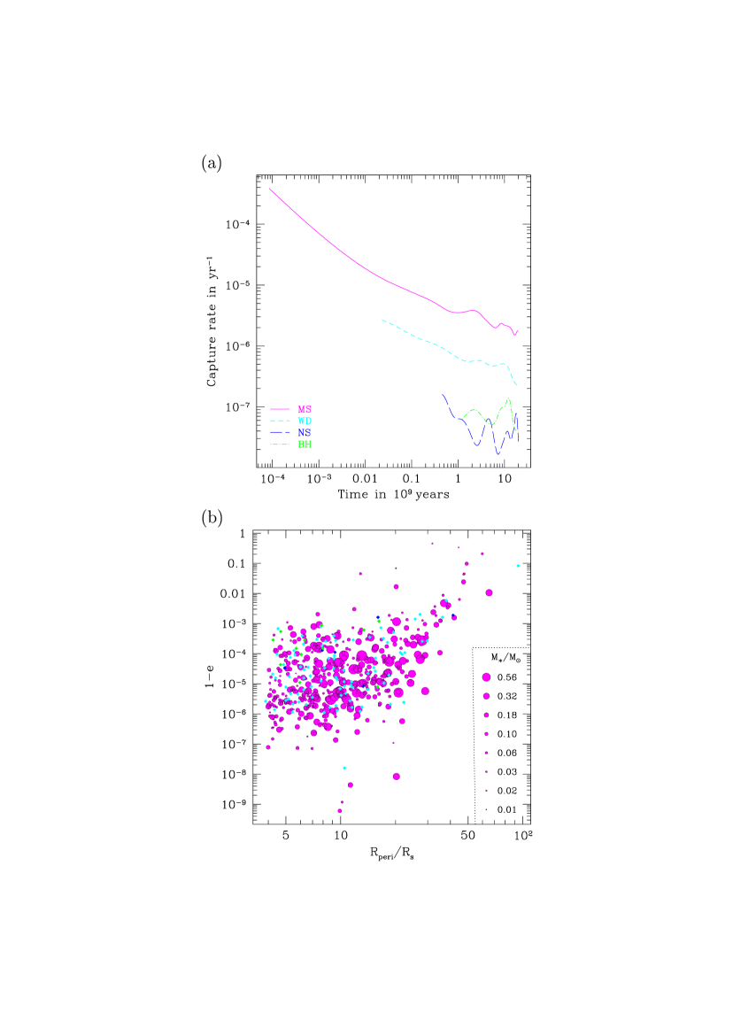
Figure 1: Captures through emission of gravitational waves for our Monte Carlo simulation of the Galactic center. (a) Evolution of the capture rates for the various stellar species. Note that only a small number of events have occurred for SBHs or NSs, hence the noisy curves. (b) Orbital parameters at capture for each event (which has a statistical weight of 65.5 stars). $e$ is the eccentricity and $R_{\mathrm{p}}$ the pericenter distance (in units of the Schwarzschild radius, $R_{\mathrm{S}}=2.5\times 10^{-7}$ pc). Only events that occurred in the first 10 Gyrs of the simulation are included. The surface of disks for MSSs is proportional to the mass of the star. Capture of compact remnants are represented with diamonds.

In Fig. 1a, we show the capture rates as a function of time. As captures are rare, we have integrated the evolution of the nucleus over many billion years to improve statistics. However, over such a long time scale, the nucleus model experiences a relatively important evolution. Most notably, significant mass segregation occurs. At the end of the simulation, the density is dominated by SBHs (which represent only 2 % of the stellar mass) in the region interior to $\sim 0.15\,$pc while the density of MSSs has decreased from a steep $\rho_{\ast}\propto R^{-1.7}$ to a milder $R^{-1.3}$ peak. This explains the steady decrease in the MSS capture rate. Given its efficiency, mass segregation should in principle be introduced from the beginning of the simulation, which is unfortunately impossible for lack of observational constrains and adequate cluster models. Anyway, it is clear that the predicted MSS capture rate is in excess of $2\times 10^{-6}\,\mathrm{yr}^{-1}$ and may be as high as a few $10^{-5}\,\mathrm{yr}^{-1}$. For WDs, the rate is a few $10^{-7}\,\mathrm{yr}^{-1}$ and around $5\times 10^{-8}\,\mathrm{yr}^{-1}$ for NSs and SBHs. These latter values are based on a small number of events and have low statistical significance. In Fig. 1(b), the initial orbital parameters are reported for all captures. One sees that orbits are very elongated, as predicted, with very small pericentre distances. Previous, analytical, studies did not address the capture of MSSs. They predicted a WD capture rate ranging from $10^{-8}\,\mathrm{yr}^{-1}$ (Hils & Bender 1995; Ivanov 2002) to $10^{-7}\,\mathrm{yr}^{-1}$ (Sigurdsson & Rees 1997). Explaining why these estimates are different from each other and from our result is beyond the scope of this letter as it would require a lengthy discussion of the different nucleus models and various treatments of the physics in these papers. We note that our WD rate is similar but larger than that of Sigurdsson & Rees (1997) while these authors predict an initial SBH capture rate some three orders of magnitude larger than ours!

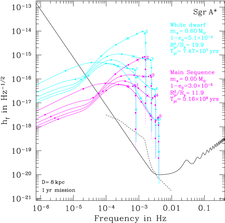
Figure 2: Gravitational signal for two events from our Sgr A^∗simulation, a WD and a low-mass MSS. We plot the amplitude versus frequency for the 5 first Fourier components of the quadrupolar radiation (Pierro et al. 2001). We use $h_{f}\stackrel{{\scriptstyle\mathrm{def}}}{{=}}h^{\mathrm{rms}}\sqrt{T_{\mathrm{obs}}}$ where $T_{\mathrm{obs}}$ is the effective duration of observation at frequency $f$, i.e., the mission duration (one year) if the signal is stable over that period. The sharp drop in the signal amplitude at the end of the evolution is due to either the time left before swallowing or the characteristic time for frequency increase, $f(\mathrm{d}f/\mathrm{d}t)^{-1}$, being shorter than the mission duration. The crosses represent the position 1000 years before plunge through the horizon. Other ticks are for positions $10^{6}$, $10^{5}$, $10^{4}$, 100, 10, 1 year, 1 month and 1 day before plunge. The segments in dotted line for the MSS correspond to $R_{\mathrm{p}}<R_{\mathrm{d}}$, a regime where tidal disruption should have occurred. The solid V-shaped curve represents LISA’s intrinsic noise ($\mathrm{SNR}=1$, Larson et al. 2000). The dashed line is an estimate of the confusion noise due to unresolved WD binaries in our Galaxy (Bender & Hils 1997).

During the course of the MC simulations, captured stars are immediately removed from the cluster. Their initial orbital parameters being known, we come back to this data and compute the inspiralling and concomitant gravitational waves emission (Pierro et al. 2001; Glampedakis et al. 2002). To illustrate this, in Fig. 2, we plot the evolution of the frequency and amplitude of the lowest five harmonics of the emitted waves for typical WD and MSS events. The WD would be detectable during a few $10^{5}$ years and the MSS for nearly $10^{6}$ years. NSs and a SBHs typically have shorter detectability durations. Multiplying these times by the respective capture rates, one gets rough estimates for the expected average number of LISA sources at the Galactic center. However, the MC data permits more precise determinations through the following method. For each event $i$, we computed the evolution of the 20 first harmonics of the rms amplitude and selected at each time the one with the highest LISA signal-to-noise ratio (SNR). Then we compute $T_{i}^{(\mathrm{detec})}(s)$, the time during which there is a harmonic with SNR larger than $s$. Finally, we get the expected number of sources with a harmonic component stronger than SNR $s$ by summation,

$$N^{(\mathrm{detec})}(s)=\frac{N_{\ast}}{N_{\mathrm{p}}}\frac{1}{\Delta T_{\mathrm{simul}}}\sum_{i=1}^{N_{\mathrm{events}}}\,T_{i}^{(\mathrm{detec})}(s).$$ (4)

The summation is realized over all the $N_{\mathrm{events}}$ events that occurred during some given time interval $\Delta T_{\mathrm{simul}}$.

Fig. 3 is the result of this computation. To have reasonable statistics, we set $\Delta T_{\mathrm{simul}}=10^{9}$ yrs for MSSs and WDs and $2\times 10^{10}$ yrs for NSs and SBHs. The most striking results concern MSSs. Even though complete tidal disruption has been assumed when the particle reaches $R_{\mathrm{d}}$, the predicted number of sources with $\mathrm{SNR}\geq 10$ is of order 3-5. If sources with SNR of 3 can be detected, then LISA should be able to observe of order 10 MSSs orbiting the Sgr A^∗ MBH. Note that for such long-lived sources, the SNR is proportional to the square root of the mission duration, likely to exceed one year.

4 Discussion

A major concern regarding this result is the role of tidal interactions which may enter the game before they are strong enough to disrupt a star in a single passage. Tides are raised at each pericentre passage, converting some orbital energy into stellar pulsation. These oscillations dampen into heat through mechanisms and on time scales that are still uncertain (McMillan et al. 1987; Kumar & Goodman 1996). Conservatively, we assume complete dissipation, thus disregarding the possibility of energy being transfered back from the oscillations to the orbital motion at next periastron passage, and ineffective radiation of this energy. The ratio of the amount of energy to be dissipated (either by gravitational waves or tides) to reach a relativistic detectable orbit, to the star’s self-binding energy is of order $(R_{\mathrm{S}}/R_{\mathrm{p}})(c/V_{\ast})^{2}(1-e)\gg 1$ where $V_{\ast}\approx 600\,\mathrm{km\,s}^{-1}$ is the escape velocity from the stellar surface. Consequently, with our assumptions, tidal dissipation cannot influence the orbit without first strongly affecting the stellar structure. Hence, to get a (over)estimate of the impact of tidal interactions in reducing the expected number of detectable stars, we computed for all capture events the tidal energy pumped into the star at each periastron passage, assuming $e\simeq 1$ and using the $n=1.5$ polytrope model from McMillan et al. (1987). When the accumulted energy reached 20 % of the self-binding energy, the star was considered disrupted. Recomputing $N^{(\mathrm{detec})}(s)$ with this pessimistic procedure, we still get of order 0.5–2 and 4–8 MSS sources with $\mathrm{SNR}\geq 10$ and $\mathrm{SNR}\geq 3$, respectively, see Fig. 3. We conclude that tidal interactions can potentialy reduce the number of sources significantly but probably not supress them completely.

We have tested the robustness of our result to several other aspects of the modeling, through a series of lower resolution simulations ($N_{\mathrm{p}}=10^{6}$). Interestingly, our conclusions are not affected if we assume a constant stellar formation rate during the $10^{10}\,$years preceding the beginning of the simulation. Observations of the Arches cluster, close to the Galactic center, are hinting to an IMF exponent of $\alpha\simeq 1.65$ for $M_{\ast}>10\,M_{\odot}$ (Figer et al. 1999). If we adopt $\alpha=1.65$ for stars more massive stars than $8\,M_{\odot}$, the capture rate is slightly lower. With the extreme assumption that $\alpha=1.65$ above $0.5\,M_{\odot}$, a very SBH-rich population is formed. After a few billion years, they dominate the central pc from which they have expelled most of the MSSs whose capture rate is reduced by a factor of 3. Modifications of the low-mass part of the IMF have direct consequences because only stars less massive than $\sim 0.6\,M_{\odot}$ may be detected before tidal disruption. The IMFs with the largest or lowest proportion of low mass stars that are still compatible with local observations (Kroupa 2001) lead to a number of predicted MSS sources higher by 40-80 %, respectively lower by of order 25 %.

Only low mass MSSs contribute as more massive but less denser ones suffer from early tidal disruption. Hence, the MSS signal would be too weak to be detected from distant galaxies. A MS source would only be marginally detectable during of order $10^{3}$ years if located in the Virgo cluster which is too short to ensure a significant detection probability. Local group galaxies are probably ruled out as well. The BH at the center of M 31 has a mass of a few $10^{7}\,M_{\odot}$ so that the frequency of gravitational waves would be too low. Detailed simulations for M 32 yield a probability for a MS source with SNR above 1 of order 0.3–0.5 only. If massive BHs are present in dwarf galaxies or globular clusters (Gebhardt et al. 2002; Gerssen et al. 2002) and their masses follow the well known correlation with the velocity dispersion of the host galaxy (Tremaine et al. 2002), they impose too intense tidal forces in their vicinity. To summarize, captured MSSs should be detected at the Galactic center, many $10^{5}$ years before plunge, but all other sources are predicted to be compact remnants in galaxies at distances of a few hundreds of Mpc, during the last few months or years of inspiral.

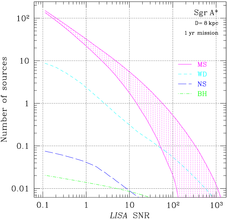
Figure 3: Expected number of sources of gravitational waves at the Galactic center. This figure shows the number of MSSs, WDs, NSs and SBHs predicted to produce a signal above a given signal-to-noise ratio ($\mathrm{SNR}$). For MSSs and WDs, the capture events that occurred in the first $10^{9}$ years of our Monte Carlo simulation have been included in the computation (95 and 11 events respectively). For NSs and BHs, we used the first $2\times 10^{10}$ years (13 and 22 events). The orbital evolution of each captured star, as driven by emission of gravitational radiation around a non-spinning black hole, has been integrated down to plunge instability or tidal disruption (Glampedakis et al. 2002) and, at each time, we select the Fourier component of the quadrupolar radiation (Pierro et al. 2001) yielding the highest SNR. The upper curve for MSSs is obtained when tidal heating is neglected. The lower curve corresponds to a pessimistic estimate of the decrease in the number of sources due to tidal heating, as described in the main text (the number of contributing events is reduced to 27).

References

- Alexander (1999) Alexander, T. 1999, ApJ, 527, 835
- Bender & Hils (1997) Bender, P. L. & Hils, D. 1997, Classical and Quantum Gravity, 14, 1439
- Binney & Tremaine (1987) Binney, J. & Tremaine, S. 1987, Galactic Dynamics (Princeton University Press)
- Chabrier & Baraffe (2000) Chabrier, G. & Baraffe, I. 2000, ARA&A, 38, 337
- Danzmann (2000) Danzmann, K. 2000, Advances in Space Research, 25, 1129
- Figer et al. (1999) Figer, D. F., Kim, S. S., Morris, M., Serabyn, E., Rich, R. M., & McLean, I. S. 1999, ApJ, 525, 750
- Freitag (2001) Freitag, M. 2001, Classical and Quantum Gravity, 18, 4033
- Freitag & Benz (2001) Freitag, M. & Benz, W. 2001, A&A, 375, 711
- Freitag & Benz (2002) —. 2002, A&A, 394, 345
- Gebhardt et al. (2002) Gebhardt, K., Rich, R. M., & Ho, L. C. 2002, ApJ, 578, L41
- Genzel et al. (2000) Genzel, R., Pichon, C., Eckart, A., Gerhard, O. E., & Ott, T. 2000, MNRAS, 317, 348
- Gerssen et al. (2002) Gerssen, J., van der Marel, R. P., Gebhardt, K., Guhathakurta, P., Peterson, R. C., & Pryor, C. 2002, AJ, 124, 3270
- Ghez et al. (2000) Ghez, A. M., Morris, M., Becklin, E. E., Tanner, A., & Kremenek, T. 2000, Nat, 407, 349
- Glampedakis et al. (2002) Glampedakis, K., Hughes, S. A., & Kennefick, D. 2002, Physical Review D, 66, 64005
- Glampedakis & Kennefick (2002) Glampedakis, K. & Kennefick, D. 2002, Physical Review D, 66, 44002
- Hénon (1973) Hénon, M. 1973, in Dynamical structure and evolution of stellar systems, Lectures of the 3rd Advanced Course of the Swiss Society for Astronomy and Astrophysics (SSAA), ed. L. Martinet & M. Mayor, 183–260
- Hills (1975) Hills, J. G. 1975, Nat, 254, 295
- Hils & Bender (1995) Hils, D. & Bender, P. L. 1995, ApJ, 445, L7
- Ivanov (2002) Ivanov, P. B. 2002, MNRAS, 336, 373
- Kormendy & Gebhardt (2001) Kormendy, J. & Gebhardt, K. 2001, in 20th Texas Symposium on relativistic astrophysics, ed. H. Martel & J. C. Wheeler, 363
- Kroupa (2001) Kroupa, P. 2001, MNRAS, 322, 231
- Kumar & Goodman (1996) Kumar, P. & Goodman, J. 1996, ApJ, 466, 946
- Larson et al. (2000) Larson, S. L., Hiscock, W. A., & Hellings, R. W. 2000, Physical Review D, 62, 062001
- Lauer et al. (1998) Lauer, T. R., Faber, S. M., Ajhar, E. A., Grillmair, C. J., & Scowen, P. A. 1998, AJ, 116, 2263
- McMillan et al. (1987) McMillan, S. L. W., McDermott, P. N., & Taam, R. E. 1987, ApJ, 318, 261
- Miralda-Escudé & Gould (2000) Miralda-Escudé, J. & Gould, A. 2000, ApJ, 545, 847
- Peters (1964) Peters, P. C. 1964, Physical Review, 136, 1224
- Peters & Mathews (1963) Peters, P. C. & Mathews, J. 1963, Physical Review, 131, 435
- Pierro et al. (2001) Pierro, V., Pinto, I. M., Spallicci, A. D., Laserra, E., & Recano, F. 2001, MNRAS, 325, 358
- Rees (1988) Rees, M. J. 1988, Nat, 333, 523
- Schödel et al. (2002) Schödel, R. et al. 2002, Nat, 419, 694
- Sigurdsson & Rees (1997) Sigurdsson, S. & Rees, M. J. 1997, MNRAS, 284, 318
- Thorne (1998) Thorne, K. S. 1998, in Black Holes and Relativistic Stars, ed. R. M. Wald, 41
- Tremaine et al. (2002) Tremaine, S. et al. 2002, ApJ, 574, 740
- Tremaine et al. (1994) Tremaine, S., Richstone, D. O., Byun, Y., Dressler, A., Faber, S. M., Grillmair, C., Kormendy, J., & Lauer, T. R. 1994, AJ, 107, 634