Constraints on the Cluster Environments and Hot Spot Magnetic Field Strengths of the Radio Sources 3C 280 and 3C 254

Abstract

We present new Chandra Observatory observations together with archival Hubble Space Telescope and radio observations of 3C 254, a radio quasar at $z=0.734$, and 3C 280, a radio galaxy at $z=0.996$. We report the detection of X-ray and possible HST optical counterparts to the radio hot spots in 3C 280 and of an X-ray counterpart to the western radio hot spot in 3C 254. We present constraints on the presence of X-ray clusters and on the magnetic field strengths in and around the radio hot spots for both targets. Both sources were thought to be in clusters of galaxies based on reports of significant extended emission in ROSAT PSPC and HRI images. The exquisite spatial resolution of the Chandra Observatory allows us to demonstrate that these sources are not in hot, massive clusters. The extended emission seen in ROSAT observations is resolved by Chandra into point sources, and is likely to be X-ray emission associated with the radio hot spots of these sources, with possible additional contributions from unrelated point sources. The intergalactic medium around these sources could be dense, but it is demonstrably not dense and hot. We conclude that radio sources are not reliable signposts of massive clusters at moderately high redshifts. We present measurements of the X-ray and optical fluxes of source features and discuss what physical processes may give rise to them. X-ray synchrotron emission could explain the radio, optical, and X-ray hot spot fluxes in 3C 280; this would require continuous acceleration of electrons to high Lorentz factors since the synchrotron lifetime of relativistic electrons that could produce the X-ray emission would be of order a human lifetime. Synchrotron self Compton (SSC) emission with or without inverse Compton (IC) emission due to scattering of the cosmic microwave background radiation can also explain the X-ray emission from the hot spots, though these most likely would require that some other physical process be invoked to explain the optical emission seen in 3C 280. High spatial resolution radio data with broad frequency coverage of the radio hot spot regions is needed to determine which physical process is responsible for the detected X-ray emission, and to provide much tighter constraints on the magnetic field strength of the hot spot plasma. We summarize our current constraints on the magnetic field strengths in and around the hot spots of 3C 254 and 3C 280.

1 Introduction

Since radio sources are visible from across the universe, understanding the connections between their observed properties and their physical conditions allows us to probe the environment and physics of galaxies billions of years ago. Radio sources are thought to inhabit regions of high galaxy density because of an excess of companions (e.g. Pascarelle et al. 1996; Le Fevre et al. 1996) and large rotation measures which could arise from hot, magnetized cluster gas (Carilli et al. 1997.) Astronomers have speculated that the most distant radio sources evolve into massive ellipticals (e.g. Pentericci et al. 1999); De Vries et al. (2000) show that the galaxy hosts are likely to be giant elliptical galaxies. Best et al. (1997ab) showed that magnitudes, colors, and profiles of 3CR radio galaxies at $z\sim 1$ are consistent with those of a $M\sim 5\times 10^{11}{\rm M_{\odot}\,yr^{-1}}$ elliptical with a formation redshift of 3-5. The closest example of such a system is Cygnus A. For reference, Cygnus A is a powerful radio galaxy inhabiting and interacting with the intracluster medium (ICM) of a relatively rich cluster of galaxies with an X-ray bolometric luminosity of $L_{x}\sim 6.2\times 10^{44}{\rm erg\,s^{-1}}$ (converted from a 2-10 keV luminosity of $L_{x}\sim 3.5\times 10^{44}{\rm erg\,s^{-1}}$), and X-ray temperature $T_{x}\sim 7.7$ keV (Smith et al. 2002.)

In this work, we observed two powerful FRIIb radio sources. An FRIIb source is defined as an edge-brightened, classical double radio source with a quite regular (cigar-like) shaped radio bridge region, and is also classified as a type 1 FRII source by Leahy & Williams (1984). FRIIb sources, described in some detail by Daly (2002), typically have radio powers at least a factor of 10 above the classical FRI-FRII break, and are found almost exclusively at relatively high-redshift (with the well-known exception, Cygnus A). For FRIIb sources, it is thought that the ram pressure confinement of the radio lobe might be used to estimate the ambient gas density using radio data alone, as was done by Carilli et al (1991) for Cygnus A, Perley & Taylor (1991) for 3C295, Wellman, Daly, & Wan (1997; WDW97 hereafter) for a sample of 22 FRIIb sources, and Guerra, Daly, & Wan (2000) for 6 FRIIb sources. A comparison of radio predicted ambient gas densities with X-ray determined ambient gas densities suggests that the magnetic field strength in the radio bridges of 3C 295 and Cygnus A are about 1/4 of the minimum energy value (Perley & Taylor 1991; Carilli et al. 1991).

If the ram pressure method of determining ambient gas densities were confirmed to be reliable by an X-ray assessment of the ambient gas densities, then we might be able to use the radio data to ascertain the density of the ICM at higher redshifts where the X-ray emission is nearly impossible to detect with current technology. Such a method would be complementary to Sunyaev-Zel’dovich (SZ) techniques since, in general, SZ imaging is more difficult near powerful radio sources. The properties of the ICM at high redshifts, insofar as they reveal the virial mass of the cluster, provide important constraints on models of evolution of clusters and of large scale structure, strongly constraining $\Omega_{matter}$ (e.g. Peebles, Daly, & Juskiewicz 1989; Donahue et al. 1998, 1999; Donahue & Voit 1999; Henry 2000, 1997; Eke et al. 1998; Borgani et al. 2002).

In order to test this method of assessing densities, we observed two very powerful, extended, classical double radio FRIIb sources, 3C 254 and 3C 280. Both of these sources had strong indications of extent in X-ray images from studies using ROSAT (Hardcastle & Worrall 1999; Crawford et al. 1999). The excellent spatial resolution of the Chandra X-ray Observatory allows us to distinguish between the compact emission from a central point source and hot spots from extended emission from a thermal, extended gaseous halo gravitationally confined by the potential associated with a cluster of galaxies. Typical clusters of galaxies have ICM luminosities of $L_{x}\sim 10^{43-45}{\rm erg\,s^{-1}}$ and gas temperatures of $T_{x}\sim 2-15$ keV. A hot intracluster medium has been detected around at least some distant 3CR radio galaxies, using Chandra’s imaging detectors. 3C294 at $z=1.786$ was found to have diffuse emission of $\sim 5$ keV and a rest-frame $0.3-10$ keV X-ray luminosity of $4.5\times 10^{44}h_{50}^{-2}$ erg s^-1 (Fabian et al. 2001). 3C295 ($z=0.47$) has a $5$ keV ICM, detected out to $1h_{50}^{-1}$ Mpc with Chandra (Allen et al. 2001). 3C220.1 ($z=0.62$) is contained within a $5$ keV ICM detected with Chandra with a rest-frame X-ray luminosity (0.7-12.0 keV) of $5.6\times 10^{44}{\rm erg\,s^{-1}}$ (Worrall et al. 2001). Despite the detections of clusters around other radio sources and the early assessments of extent in 3C 280 and 3C 254, in this work we find that neither of these sources is in a cluster of any significance ($L_{x}\gtrsim 3\times 10^{43}$ erg s^-1.) We discuss our X-ray observations, our limits on extended X-ray flux, and what inferences may be made regarding the ICM surrounding these sources.

However, we also detect significant emission from X-ray counterparts of the radio hot spots in both sources. In this paper, we describe the two targets of our studies in §2. We outline the details of the Chandra observations and analysis in §3. We briefly discuss our reduction and analysis of HST data in §4. The limits placed on the existence of the X-ray clusters and the density profiles of each system are contained in §5.1 and §5.2, along with a review of the archival ROSAT data in §5.3. In §6.1, we present useful relations for computing the expectations for synchrotron self-Compton (SSC) processes in hot spots, and apply them to our observations. In §6.2 we discuss the contribution of synchrotron to the X-ray and possible optical emission; in §6.3 we do the same for inverse Compton (IC) scattering of the microwave background. In all sections we place constraints on the magnetic field. In §7, we summarize our conclusions regarding the physical environments of the radio sources, the physical processes causing the hot spots, and the magnetic fields in those hot spots.

For the purposes of comparing luminosities and length scales between this work and previous X-ray research, we assume $H_{0}=50h_{50}$ km s^-1 Mpc^-1 and $q_{0}=0.0$, implying an angular distance scale of $10.885h_{50}^{-1}$ kpc arcsecond^-1 for 3C 280 and $9.700h_{50}^{-1}$ kpc arcsecond^-1 for 3C 254. For reference, here are the angular distance scales and luminosity conversion factors for the currently most fashionable cosmology of $H_{0}=65$ km s^-1 Mpc^-1, $\Omega_{M}=0.3$, and $\Omega_{\Lambda}=0.7$: the angular distance scale are $8.616h_{50}^{-1}$ kpc arcsecond^-1 for 3C 280 and $7.838h_{50}^{-1}$ kpc arcsecond^-1 for 3C 254. The luminosities quoted in this paper would decrease by a factor of the luminosity distance $D_{L}^{2}$: 0.63 for 3C 280 and 0.65 for 3C 254.

2 Individual Sources

3C 254 is a radio-loud FRII quasar with $z=0.734$ (Spinrad et al. 1985) at 11h 14m 38.5s +$40\arcdeg$ 37$\arcmin$ 20$\arcsec$ (J2000). The radio source is very asymmetric, with its shortest hot spot-nuclear separation on the eastern side. Owen & Puschell (1984) showed that the eastern lobe is extended roughly perpendicular to the source axis. An overdensity of galaxies near the source suggests the environment is a cluster or a group (Bremer 1997). This overdensity consists of seven objects within $10\arcsec$ ($97h_{50}^{-1}$ kpc), with magnitudes within 3-5 magnitudes that of the central galaxy. The magnitudes are consistent with passively evolving $L^{*}$ galaxies at $z=0.734$ with $z_{formation}>2$ (Bremer 1997).

3C 280 is an FRII radio galaxy with $z=0.996$ (Spinrad et al. 1985) at 12h 56m 57.1s $+47\arcdeg$ 20$\arcmin$ 20$\arcsec$ (J2000). It is one of the most powerful FRIIs known at radio frequencies. It has an extended ($11\arcsec$) emission line nebula ([OII]3727Å), with a central peak and a loop around the eastern radio lobe (McCarthy et al. 1987).

Best’s (2000) K-band images of both of these sources suggest a richness class 0 environment. At low redshift, richness class 0 clusters of galaxies tend to have X-ray luminosities between $10^{43-44}{\rm erg\,s^{-1}}$.

ROSAT observers reported extended emission from both of these sources (Hardcastle & Worrall 1999; Crawford et al. 1999; Worrall et al. 1994). For 3C 254, residuals with extent of $30-60\arcsec$ were estimated from PSPC images (Hardcastle & Worrall 1999). Crawford et al. (1999) identifies excess emission out to at least $15\arcsec$ (145 kpc $h_{50}^{-1}$) in 3C 254, with 12-19% of the total X-ray luminosity in extended emission, corresponding to $L_{x}\sim 5-9\times 10^{44}h_{50}^{-2}{\rm erg\,s^{-1}}$. For 3C 280, Worrall et al. (1994) reported PSPC evidence for a cluster extent of $18-65\arcsec$ ($200-700h_{50}$ kpc). Hardcastle & Worrall (1999) reported rest-frame 2-10 keV X-ray luminosities of $1.3\times 10^{45}h_{50}^{-2}{\rm erg\,s^{-1}}$ and $2.8\times 10^{44}h_{50}^{-2}{\rm erg\,s^{-1}}$ for 3C 254 and 3C 280 respectively. Correspondingly, Hardcastle & Worrall (2000) estimated rough ICM pressures of $\sim 7\times 10^{-12}$ ($\sim 8\times 10^{-13}$) erg cm^-3 for 3C 254 (3C 280), assuming 7.7 (5.0) keV gas temperatures. In § 5.3, we have re-analyzed these ROSAT data for comparison purposes.

3 Chandra Observations and Analysis

Both 3C 280 and 3C 254 were observed with the Chandra ACIS-S in VFAINT datamode and TIMED readmode. We reprocessed the level 1 events file using updated gain maps from CALDB v2.9 (2001-10-22) and CIAO2.2. Only events with the ASCA grades of 0, 2, 3, 4, and 6 and a status$=0$ (“clean”) were used in the subsequent analyses.

3C 254 was observed for 29,668 kiloseconds (all corrections applied) on March 26, 2001. The observation was uncontaminated by flare activity, so the good time intervals, as supplied by the original pipeline, were used to extract the final clean data.

3C 280 was observed for 63,528 (standard good time intervals) on August 27, 2001. A light curve of the background light between 0.3-8.0 keV reveals several flares. Even the “quiescent rate” for the observations varied several times. For analysis of flare-free “clean” data, we only use the 18,944 seconds of data near the beginning of the observation, particularly for the analysis of extended sources. The signal to noise estimates of point sources in these clean data are extremely compromised relative to the total, so for analysis of the point sources, which are relatively unaffected by background (usually less than $\sim 10\%$ of the total count rates), we also analyzed the full data set for 3C 280. For the point sources, the count rates and spectra from the full data set are statistically consistent with those extracted from the clean data, and therefore, for the spectral fits (only for the purposes of improving flux estimates of the point sources and for the approximation of their broadband spectra) were done with the full data set of 63,528 seconds.

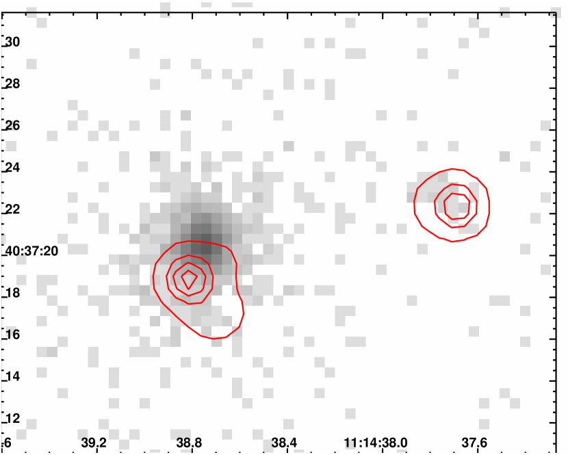
Figure 1: Radio contours overlaid on the X-ray greyscale images for 3C 254 and 3C 280. The 3C 254 radio intensity map was made with the VLA by Liu, Pooley, & Riley (1992), observed on March 21, 1989 with a resolution of $1.25\arcsec\times 1.25\arcsec$ at 4885.10 MHz.

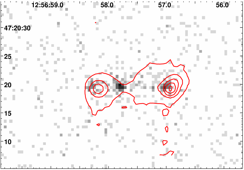
Figure 2: Radio contours overlaid on the inverse greyscale image of the Chandra X-ray image for 3C 280. The 3C 280 radio map was obtained from Liu, Pooley, & Riley (1992). The radio observation was made with the VLA on January 21, 1989, at 1464.90 MHz, with $1.20\arcsec\times 1.20\arcsec$ resolution.

For 3C 254, we locate the position of a powerful central X-ray source, confirming the very short projected distance between the nuclear source and the western radio lobe seen by Owen & Puschell (1984). The eastern radio hot spot was not detected (it may be too close to the central source), but the western hot spot has a faint X-ray counterpart (Figure 1). For 3C 280, we detect both the western and eastern hot spots as well as the nuclear source in the X-ray (Figure 2). There may be faint emission associated with the bridge; however, estimates of contamination from the scattering wings of the three point sources shows this emission to be very uncertain, whether evaluated in the restricted or the full dataset. Neither 3C 254 nor 3C 280 (using only the cleaned dataset) showed any evidence for the putative cluster sources expected from the previous analyses of the ROSAT data for these same sources. Discussion of the Chandra limits are in § 5.2.

For the nuclei and the hot spot sources, we used a 4 pixel (1 pixel = 0.4920”) radius aperture to extract counts. A 4 pixel radius encircles approximately 90% of the energy at 1.7 keV, a correction which is not included in the fluxes and luminosities reported in Table 1. We also extracted a count estimate for the bridge region of 3C 280, excluding the 3 point sources, for a region of $35\times 10$ pixels ($17\farcs 22\times 9\farcs 42$), elongated exactly east-to-west, with 3 $r=4$ pixel regions excluded for a total area of of 150 square arcseconds. The background-subtracted count rates (0.3-10.0 keV) inside those apertures and the percentages of the total count rates in background counts are reported in Table 1. For each source, a PI spectrum was extracted and binned to at least 15 counts per PI bin. We used XSPEC v11.1 to fit a power law spectrum to the $0.3-8.0$ keV data, with Galactic absorption, fixed at $1.2\times 10^{20}$ cm^-2 for 3C 280 and $1.8\times 10^{20}$ cm^-2 for 3C 254 (Dickey & Lockman, 1990; Stark et al. 1992). The fit range is approximate, because of the width of the bins in each spectrum. A power law absorbed by the expected Galactic absorption adequately described the spectrum for all of these sources in terms of $\chi^{2}$. A thermal spectrum could also be fit to most of the spectra, except for those of the central sources of 3C 254 and 3C 280. The central source of 3C 280 seems to be unusually flat with a best-fit spectral index near 0.0; the cleaned data were consistent with that result, with a truncation near 8 keV, but the poor statistics of that flare-affected data limit our ability to confirm the power law index from the full dataset – the data from the clean set are consistent with the fit from the full, but cannot be used for an independent measurement of the slope of the power law.

The central source of 3C 254 was affected by pile-up at about the $10\%$ level. Pile-up flattened the observed spectrum and produced a broad “emission” feature at around 2 keV. We first fit the spectrum without a pileup model to obtain a best first-guess estimate of the slope and normalization of $\alpha=1.3$ and normalization of $1.4\times 10^{-4}$ respectively (the normalization units are photons keV^-1 cm^-2 s^-1 at 1 keV). The inclusion of the pile-up correction in XSPEC induces unstable fitting in local minima unless a reasonable first-guess is provided. With the XSPEC pileup model, with frame-time set to 3.2 seconds, maximum number of piled-up photons set to 5, $\alpha_{pileup}=0.5$ and $g0=1$ (pileup model parameters fixed at recommended values), the best fit slope (photon index) was $\alpha=1.8\pm 0.1$, $N_{H}=3.2\times 10^{20}(1.8-6.2)$ cm^-2, and normalization of $4.9\times 10^{-4}$. The reduced $\chi^{2}=1.2$ for this fit with 161 degrees of freedom obtains a null hypothesis probability of 0.05. This power law index somewhat exceeds the best-fit power-law index from ASCA data of $\alpha=1.67\pm 0.04$ obtained by Sambruna, Eracleous, & Mushotzky (1999), but the estimates overlap at the 90% uncertainty level, which, given the uncertainties in the pile-up model, is not bad.

For 3C 280 and 3C 254, thermal spectra from a gas with $kT\sim 2$ keV and metallicity of $\sim 30\%$ solar also adequately described the spectrum for the hot spot sources. The excess counts from the bridge of 3C 280 could be described by a cooler thermal spectrum of $1.3^{+0.2}_{-0.6}$ keV (with no constraints on the metallicity). As noted earlier, this source is likely to be heavily contaminated by scattered light from the hot spots and the nucleus so its flux is highly uncertain. Also, since it is not a point source, its spectral properties can be affected by how the background is handled. The inferred broad-band fluxes and luminosities for all the sources depend somewhat on the assumption of a spectral model, whether power-law or thermal, so we report those properties under both model assumptions in Table 1 for those sources with insufficient signal to distinguish between the two spectral models.

4 Hubble Space Telescope Observations and Measurements

In order to detect or place limits on optical synchrotron emission from the radio hot spots, we retrieved HST Wide Field Planetary 2 (WFPC2) data from the HST Archive for both sources. We used co-added and cosmic-ray rejected data from both the CADC and the ECF HST data archives, and compared photometry from those co-added data with that from individual observations retrieved from the HST data archive. The co-addition process (with averaging) obtained consistent photometry for these observations. The gain for all observations was 7.0 electrons per DN (data number). The observations were reduced with standard calibration software using the most recent calibration files, switches, and software. No astrometric shifts were applied to the HST data. The IRAF/STSDAS task invmetric was used to derive the x and y positions corresponding to the right ascension and declination of the X-ray hot spots.

The target 3C 254 was observed in a Planetary Camera (PC) snapshot program in both the F702W (R-band) and the F555W (V-band) filters. The nucleus was saturated, but the host galaxy was detected (Lehnert et al. 1999). We do not detect a counterpart for the radio hot spots in either image. We report a $3\sigma$ upper limit for a $1\arcsec\times 1\arcsec$ aperture centered on the X-ray position of the western hot spot for the F702W observation in Table 2.

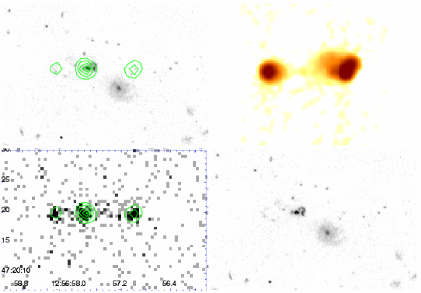
Figure 3: This figure shows four observations of 3C 280 in the optical, radio, and X-ray, displayed with the same scale and orientation. The upper left figure is the HST WFPC2 image of 3C 280 with X-ray contours overlaid (sufficient to show the location of the core and the two hot spots); the lower right figure is the same grey-scale image with the X-ray contours omitted. The upper right image is the VLA radio image from Liu, Pooley, & Riley (1992); the lower left image is the X-ray image with the same X-ray contours as the upper left HST image. We frame the lower left image with the coordinate system of all 4 images. The nucleus of 3C 280 seems to be coincident with feature “a” from Ridgway & Stockton (1997).

The target 3C 280 was observed in the Wide Field Planetary Camera 2 (WFPC2), Wide Field 3, for a total of 8800 seconds in the F622W filter. Ridgway & Stockton (1997) report the unusual appearance of the central galaxy. We find two point-source features within $0\farcs 67$ and $0\farcs 45$ of the western and eastern hot spot Chandra positions, and aligned with the peaks of the radio hot spots in the Liu, Pooley, & Riley (1992) maps (Figure 3). We extracted background-subtracted aperture ($r=0\farcs 3$) photometry at the positions of the HST point sources. Using the basic flux calibration information from the header (the PHOTFLAM keyword) we converted the observed count rates (DN sec^-1) to flux densities in nJy at 6200 Å. We corrected these fluxes for geometric distortion ($\sim 1\%$) (Casertano & Wiggs 2001), charge transfer inefficiency ($\sim 2-3\%$), and aperture ($\sim 16\%$) (Whitmore & Heyer 2002; HST Data Handbook.)

The optical flux densities of these point sources are consistent with optical synchrotron emission from the radio and X-ray hot spots, but are very unlikely to be produced by synchrotron self-Compton (SSC) or inverse Compton (IC) of the cosmic microwave background (CMB). We will discuss this topic further in §6.

5 Evaluation of Extended X-ray Emission

The distribution of X-ray emission in clusters of galaxies is typically extended, with a core radius of $\sim 100-200h^{-1}$ kpc, and is centered near the center of mass of the cluster. The X-rays arise from an optically thin plasma confined by the gravitational potential of the cluster; the temperature of the gas is indicative of the depth of the potential. Cluster luminosities are typically $10^{43}-10^{45}$ erg s^-1. Cluster temperatures run between 2-15 keV and typical central densities range between $10^{-2}$ and $10^{-4}$ cm^-3. In the following section, we describe the analysis performed in order to place constraints on the presence of an extended component arising from a cluster of galaxies centered on these radio sources.

5.1 Radial Profile of 3C 254

A visual inspection of the 3C 254 X-ray image reveals a faint halo around the central bright source. Here we show this halo is consistent with being part of the point spread function (PSF) of a very bright Chandra X-ray source.

We constructed a model PSF from the library of Chandra PSFs by extracting PSFs for the on-axis position on the ACIS-S from the library for six different energies: 0.80, 1.25, 2.25, 3.50, 4.50, and 5.50 keV respectively. Based on the energies of photons in the central X-ray source of 3C 254, each PSF was weighted to construct a summed, normalized PSF. In Figure 6, the resulting radial profile of the predicted PSF is plotted against the radial profile of the central source, extracted identically. Inspection of this plot reveals that there is no detectable excess within $10\arcsec$ of the central source over the halo of a bright point source. We therefore exclude a region of radius $12\arcsec$ around the X-ray bright nuclear source of 3C 254 when placing a limit on cluster emission around this radio quasar (§5.2).

5.2 Upper Limits to Cluster Emission and to Density Profiles of Hot Gas

We used SHERPA, CIAO’s fitting engine, to fit the extended, flare-filtered data within $\sim 3h_{50}^{-1}$ Mpc for both targets between $0.3-2.0$ keV with the point sources detected by the CIAO routine wavdetect masked out (see Figure 7). For 3C 254, we also masked out a larger region ($\sim 12\arcsec$) around 3C 254 and a region around the readout streak. The $0.3-2.0$ keV energy range maximized our sensitivity to soft thermal emission while minimizing the contribution from the particle backgrounds. Images were binned by a factor of 4 ($\sim 2\arcsec$ pixels) to increase the S/N of each pixel and to reduce the computation time for fitting. Using the Cash statistic to assess the relative goodness of fit, we fit a circular beta-model profile to the observed surface brightness $S_{x}$ with the function $S_{x}=S_{0}(1+(\theta/\theta_{C})^{2})^{-3\beta+1/2}$ and a constant background. $S_{0}$ is the normalization, $\theta$ is the angular separation from a center (assumed to be aligned with the central X-ray point source), $\theta_{C}$ is the core radius, and $\beta$ is the slope of the traditional cluster beta function (typically $\sim 2/3$.) The beta-model slope $\beta$ and the core radii ($\theta_{C}$) we tested span a range of standard cluster and group values. We then derived the $3\sigma$ upper limit to the best fit central surface brightness using the SHERPA projection command (Table 3 and 4) for each pair of $\beta-\theta_{C}$ values. To infer a limit on the cluster luminosity and central density, we derive the limit on the total count rate within an aperture of radius $2h_{50}^{-1}$ Mpc, then convert that to a bolometric luminosity limit by assuming a temperature within 1.0 keV of the Markevitch (1998) $L_{x}-T_{x}$ relation. Approximate limits on $L_{bol}$ are $2.5\times 10^{43}h_{50}^{-2}$ erg s^-1, for $N_{H}=1.2\times 10^{20}~{}\rm{cm}^{-2}$ and $1.87\times 10^{20}~{}\rm{cm}^{-2}$ (Dickey & Lockman, 1990; Stark et al. 1992) for 3C 280 and 3C 254, respectively (Table 5).

We convert the central surface brightness to a central electron number density, following the derivations for the emission measure from Equation 5.68 in Sarazin (1988) where $n_{e}/n_{p}=1.209$ for a fully ionized plasma of solar abundances. For a spherically symmetric plasma, the central electron density in units cm^-3 is:

$$n_{e}=\sqrt{\frac{(n_{e}/n_{p})\,4\pi^{1/2}\,k\,(1+z)^{2}\,S_{0}\Gamma(3\beta)}{3.0856\times 10^{7}\,r_{c}\,\Gamma(3\beta-1/2)}}$$ (1)

where $r_{c}$ (core radius) is in kiloparsecs. We define $k$ here to be XSPEC normalization of a Raymond Smith (or Mekal) thermal spectrum divided by the Chandra count rate in the source spectrum. In this definition, $\int n_{e}n_{H}dV=k\times CR\times 10^{-14}/(4\pi(D_{A}(1+z))^{2})$ where $CR$ is the total count rate (counts sec^-1) from the volume $dV$, $D_{A}$ is the angular size distance to the source in $cm$, $n_{e}$ is the electron density ($cm^{-3}$), $n_{H}$ is the hydrogen density (cm^-3) and $V$ is volume in units $cm^{3}$ (XSPEC 11.1, Raymond and Smith model.) The normalization per unit count rate $k$ depends on bandpass, temperature, metallicity, and absorption column. The quantity $S_{0}$ is counts sec^-1 sr^-1. We compute the total projected emission measure along our line of sight to the cluster inside an aperture of $2h_{50}^{-1}$ Mpc, derived assuming Galactic absorption and Raymond-Smith models in XSPEC with the response matrices appropriate to the center of the ACIS-S chip.

The normalization $k$ for the 0.3-2.0 keV count rates from a 1.0 keV plasma with a 30% solar metal abundance (typical of a cluster of galaxies at $z<0.8$ (Donahue et al. 1999)) are $1.43\times 10^{-2}$ in units of XSPEC normalization per Chandra count rate (counts sec^-1) for 3C 280 and $1.08\times 10^{-2}$ for 3C 254. The conversion factor from central surface brightness (in units of counts sec^-1 arcmin^-2) to bolometric luminosity for the same plasma, $\beta=0.7$ and $r_{c}=250h_{50}^{-1}$ kpc, are $5.02\times 10^{46}h_{50}^{-2}{\rm erg\,s^{-1}}/(\rm{count\,sec^{-1}\,arcmin}^{-2}$) and $2.28\times 10^{46}h_{50}^{-2}{\rm erg\,s^{-1}}/(\rm{count\,sec^{-1}\,arcmin}^{-2}$) for 3C 280 and 3C 254 respectively.

The $3\sigma$ upper limits on the central electron density, given $\beta$, $r_{core}$, and $k(T_{x},Z_{\odot},N_{H})$, are derived using Eq. 1. In Table 5, we report $3\sigma$ limits on the bolometric X-ray luminosity ($L_{bol}$) inside $2000h_{50}^{-1}$ kpc, the central electron density ($n_{e}$), and the electron density ($n_{e}(r)$) at the hot spot radii, $r$, given $r_{core}=250h_{50}^{-1}$ kpc and $\beta\sim 0.7$ (typical of clusters of galaxies). We estimate $n_{e}(r)$ to compare to the electron density $n_{w}(r)$ computed by WDW97. We also explored the same limits for a range of $\beta=0.55-0.75$ and core radius $r_{core}=150-350h_{50}^{-1}$ kpc. All combinations of those two parameters predicted central electron densities of $\sim(2-14)\times 10^{-4}h_{50}^{1/2}$ and not much smaller densities at $78h_{50}^{-1}$ kpc (since $r<r_{core}$), where the Wellman et al. (1997a) predictions were made based on the radio sources.

WDW97 predict two sets of ambient gas densities; one set assuming minimum energy conditions to obtain the magnetic field strength in the radio bridge region, and one set assuming that the magnetic field strength in the radio bridge is about 1/4 of the minimum energy value, as suggested by comparisons of the radio and X-ray determined ambient gas densities around 3C 295 (Perley & Taylor 1991) and Cygnus A (Carilli et al. 1991). This magnetic field strength is parameterized by $b=B/B_{min}$. WDW97 assumed a value of Hubble’s constant of $100\hbox{ km s}^{-1}\hbox{ Mpc}^{-1}$. For the case $b=1$, synchrotron cooling dominates over inverse Compton cooling with the cosmic microwave background radiation, and the radio determined ambient gas density scales as $H_{o}^{12/7}$ (see the footnote to Table 4 of Guerra, Daly, & Wan 2000), so for value of $H_{o}$ adopted here, all of the ambient gas densities listed in Table 1, column 9 of WDW97 decrease by a factor of 0.3. Thus, the ambient gas density a distance of about $78h_{50}^{-1}$ kpc from the nucleus of 3C 254 is predicted to be about $1.5\times 10^{-3}\hbox{ cm}^{-3}$. The ambient gas density for the western lobe of 3C 280 at a distance of about $76h_{50}^{-1}$ kpc from the center of the radio source is predicted to be about $7\times 10^{-3}\hbox{ cm}^{-3}$, while that for the eastern lobe at a distance of about 62 kpc from the radio source center is about $2.4\times 10^{-3}\hbox{ cm}^{-3}$ for $b=1$. These ambient gas densities are significantly larger than the $3\sigma$ upper bounds provided by the Chandra data for both sources. For $n_{W}$ for 3C 254, $b=1$ estimates of $n_{W}$ could be consistent with the X-ray upper limits if $r_{c}<150h_{50}^{-1}$ and $\beta>0.7$, values that are more consistent with belonging to groups than clusters.

For the case $b=1/4$, the radio predicted ambient gas densities are consistent with the X-ray bounds for most values of $\beta$ and $r_{c}$. We report the converted densities ($n_{W}$) in Table 5 For $b=1/4$ the bridge magnetic energy density for the bridges of 3C 254 and 3C 280 are comparable to the energy density of the cosmic microwave background, so inverse Compton cooling is as important in these regions as synchrotron cooling, and the radio-predicted ambient gas density scales as $H_{0}^{20/7}$ (see the footnote to Table 4 of Guerra, Daly, & Wan 2000). For the case $b=1/4$, the predicted ambient gas densities are obtained from column 11 of Table 1 of WDW97 and multiplied by the factor 0.14 $=(0.5)^{20/7}$ to account for the value of $H_{0}$ adopted here. The radio-predicted ambient gas densities are then about $2.1\times 10^{-4}\hbox{ cm}^{-3}$ for the western lobe of 3C 254, and about $8.3\times 10^{-4}\hbox{ cm}^{-3}h_{50}^{20/7}$ for both the western and eastern lobes of 3C 280. These gas densities predicted by Wellman et al (1997a) ($n_{W}$) for $b=1/4$ are listed in Table 5. For both sources, the radio-predicted ambient gas density is consistent with the upper bound provided by Chandra for $b=1/4$.

The radio predicted ambient gas density has a very strong dependence on $H_{0}$ and thus also the coordinate (or proper) distance ($a_{0}r$) to the source. When inverse Compton cooling with CMB photons is important, the ratio of the radio determined ambient gas density $n_{W}$ to the X-ray determined value $n_{e}$ is $n_{W}/n_{e}\propto(a_{0}r)^{-2.36}\propto h_{50}^{2.36}$. If we shift from the cosmology assumed here, $H_{0}=50$ km s^-1 Mpc^-1 and $q_{0}=0$, to a cosmology with $H_{0}=65$ km s^-1 Mpc^-1, $\Omega_{m}=0.3$, and $\Omega_{\Lambda}=0.7$, the ratio between the predicted value by Wellman et al (1997a) and the $3\sigma$ upper limit from the Chandra observations is increased by a factor of about $(0.8)^{-2.36}\simeq 1.7$. This effect does not change our conclusion presented above for 3C 254, but it does affect the comparison between the radio-predicted ambient density and the upper limit on the density from the X-ray observations of 3C 280, where the radio-predicted ambient density may be in conflict with the X-ray observations at about the $1\sigma$ confidence level. The radio predicted ambient gas density is increased by the ratio of the coordinate distances, (0.8), to the power 2.86, leading to a predicted ambient gas density for 3C 280 (see Table 5) of about $(16\pm 5.5)\times 10^{-4}$ cm^-3, whereas the upper bound placed by the Chandra observations increases by a factor of the square root of the ratio of the coordinate distances, $(0.8)^{-0.5}$ to about $10\times 10^{-4}$ cm^-3.

An additional test could be made using our limits on the temperature of any putative X-ray-emitting gas distribution if the ambient gas pressure based on the radio properties of 3C 254 and 3C 280 could have been determined, as it has for many other high-redshift 3C sources (see Table 1 of Wan et al. 2000). The luminosity limits are extremely stringent for both sources, corresponding to bolometric luminosities of $\sim 3.5\times 10^{43}h_{50}^{-2}$ and corresponding temperatures $T_{x}\sim 1.5$ keV.

These observations rule out the presence of a hot, massive cluster with a bright intracluster medium for these particular radio sources. Specifically, we definitively rule out the presence of a cluster with the luminosity and distribution of X-ray plasma like the one containing Cygnus A and like that of the putative clusters associated with these sources, as inferred from ROSAT data (see more in § 5.3).

Our conclusions are consistent with the recent findings from an optical study by Harvanek & Stocke (2002) that found that FRII-selected clusters are less rich (Abell richness class 0-1) than their X-ray selected cousins, which tend to contain FRI sources exclusively. In their study, based on a review of radio structures and surrounding galactic density for 3CR radio galaxies between $z=0.15-0.65$, they conclude that radio sources with a large bending angle cannot be used as signposts for rich clusters around powerful radio sources.

5.3 ROSAT PSPC and HRI Fluxes

In this section, we compare the Chandra observations with both earlier results from the literature and with the archived ROSAT observations, in order to try to understand why clusters were reported around these objects. We find that the total fluxes measured by ROSAT and Chandra within $120\arcsec$ are in agreement for 3C 280, and that the nuclear source for 3C 254 has likely varied in the last five years. Therefore, at least for 3C 280, the extended emission inferred from the ROSAT data is explained by faint point sources.

3C 280 was observed by the ROSAT PSPC in 1997 for 47.6 kiloseconds. Worrall et al. (1994) found that the PSPC radial profile was best fit by a point source plus a $\beta$-model, although they could not constrain the core radius very well. They stated that 60% of the net counts in the 0.2–1.9 keV band were from an extended component around 3C 280 and a flux density of 1.7 nJy at 1 keV from the extended component. Although not actually given, their total flux density can be computed using quantities in Table 4 of Hardcastle & Worrall (1999). The total flux density at 1 keV is 6.2 ($\pm$ 3.6) nJy within a source radius of 120$\arcsec$ (uncertainties were high for the extended component). They also noted a possible asymmetry in the X-ray emission.

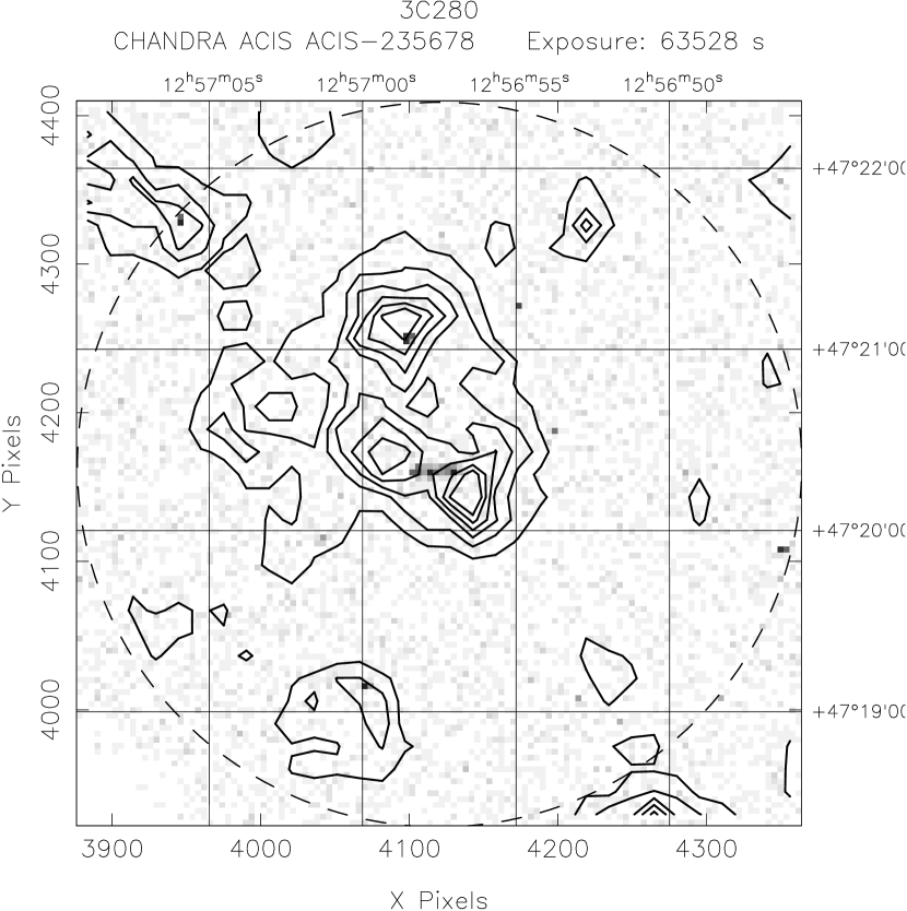
Figure 4: Chandra ACIS-S3 image (binned by 4) overlaid with ROSAT PSPC 0.5–2.0 keV X-ray contours. The contours begin at 1.5 times the background level and increase in steps of 0.5 times the background level thereafter. The dashed circle indicates the 120$\arcsec$ source radius used by Worrall et al. (1994).

Using the same PSPC data, we cleaned three episodes of high background from the data for net 42.7 kiloseconds (corrected for dead time). We adaptively smoothed the 3C 280 events with energies between 0.5–2.0 keV (the lower limits means we cut out much of the soft X-ray background) to a minimum of 10 counts in the smoothing kernel. Figure 4 shows the resulting PSPC contours overlaid on the $4\times 4$ binned Chandra 63 ks image.

The emission has at least three peaks within the $120\arcsec$ source radius used by Worrall et al. (1994). The northern peak is definitely seen in the Chandra image as a separate point source. Other, fainter sources in the Chandra image may also be contributing to the total PSPC flux. Worrall et al. (1994) considered all these emission regions as one source.

As a check, we compare the total PSPC flux within a $120\arcsec$ region around 3C 280 to the summed flux of Chandra point sources within the same region. First, we extract the PSPC spectrum for an aperture of $120\arcsec$ around 3C 280 with a background from an annulus about 3$\arcmin$-4.5$\arcmin$, masking out several sources in the background. A custom ARF and standard PSPC RMF were used; the spectrum was binned to 8 energy bins. The resulting spectrum was fit to an $\alpha=2$ power law model in XSPEC 11.2 leaving only the model normalization as a free parameter. $N_{H}$ was fixed at the Galactic value (Dickey & Lockman 1990; Stark et al. 1992). We derive a 0.5-2.0 keV flux of $2.4\pm 1.5\times 10^{-14}$ ${\rm erg\,s^{-1}\,cm^{-2}}$, which corresponds to a flux density of $6.6\pm 4.1$ nJy at 1 keV. This value is statistically the same as the 6.2 nJy 1 keV flux found by Worrall et al. (1994). A similar analysis of the ROSAT HRI data (observed for 53 ks in 1997) gives an HRI count rate of $1.1\times 10^{-3}$ ct s^-1 which corresponds to a flux of $2.2\times 10^{-14}$ ${\rm erg\,s^{-1}\,cm^{-2}}$ or 6.1 nJy at 1 keV.

The sum of the estimated flux densities from Chandra sources within $120\arcsec$ of 3C280, including five background sources, is $\sim 4.9\pm 0.6$ nJy (with an approximate $10\%$ correction for the flux outside the 4 pixel apertures). The sum of the point sources and bridge source within $120\arcsec$ of the 3C 280 nucleus is statistically consistent with but somewhat lower than the ROSAT PSPC and HRI estimates from the original data. So most, if not all the ROSAT flux can be accounted for by the point sources in the Chandra observation.

3C 254 was observed by the ROSAT PSPC for 16 ks in 1997 and with the ROSAT HRI for 29 ks in 1996. Hardcastle & Worrall (1999) report a total (extended and point-like) 1 keV flux density of $\sim 250\pm 13$ nJy. They found that the radial profiles of both the PSPC and HRI data showed evidence for extended emission, although the HRI data gave a somewhat smaller and less luminous extended component.

We analyzed the PSPC observation of 3C 254 similarly to 3C 280 and, assuming a power law index of 1.0, found a flux density at 1 keV of $168\pm 10$ nJy, somewhat smaller than the Hardcastle & Worrall estimate. Our HRI flux density is also somewhat lower at 201 nJy. However, the Chandra estimate of the 1 keV flux density is $\sim 300$ nJy, larger than either of these values. The small difference in assumed power law indices assumed (Hardcastle & Worrall 1999 assume a power law index of 0.8) does not account for the variation. The comparison between the ROSAT and Chandra fluxes shows what is likely to be long-term X-ray variability of the radio quasar.

Table 6 summarizes our ROSAT results.

6 X-ray Emission Associated with the Radio Hot Spots

The X-ray emission that is coincident with the radio hot spots could be produced by the synchrotron self-Compton process (SSC), by synchrotron radiation, by inverse Compton scattering with external photon fields, by a combination of these processes, or by some other process. SSC and synchrotron radiation are discussed in §6.1 and 6.2. Considerations of inverse Compton scattering of an external photon field, such as the cosmic microwave background radiation (CMB), allow a lower limit to be placed on the magnetic field strength of the region, which is discussed in §6.3. Constraints on the bridge magnetic field strength of 3C 280 are also discussed in this section.

6.1 The Synchrotron Self-Compton Process

Sources with Chandra detections of hot spot emission that is most likely due to SSC include 3C 295 (Harris et al. 2000), Cygnus A (Wilson, Young, & Shopbell 2000), 3C 123 (Hardcastle, Birkinshaw, & Worrall 2001) and 3C 207 (Brunetti et al. 2002).

SSC emission is most important in bright small regions, such as radio hot spots, while IC upscattering of external photons, such as those that comprise the CMB, is important in the more diffuse lobe and bridge regions of the source. The dominant mechanism in any area is determined by the ratio of the local photon energy densities. IC scattering of local synchrotron photons, known as synchrotron self-Compton emission (SSC), will dominate over scattering of ambient photons, such as those of the CMB, when the local energy density of synchrotron photons is larger than the energy density of other photon fields. For a uniform spherical synchrotron emitting region with bolometric luminosity L, radius r, and volume V, the local photon energy density is approximately $u_{s}\approx 0.75Lr/(cV)$ (Band & Grindlay 1985). The bolometric luminosity $L=\int L_{\nu}d\nu$ can be written in terms of a bolometric correction factor $\kappa_{\nu}$, where $\kappa_{\nu}=L/(L_{\nu}\nu)=f/(f_{\nu_{o}}\nu_{o})$; $f$ is the total flux, $f=\int f_{\nu_{o}}\nu_{o}$, and $f_{\nu_{o}}$ is the flux density detected at frequency $\nu_{o}$. The energy density of synchrotron photons in a region with diameter $2r$ and corresponding angular diameter $\theta$ is $u_{s}\approx(9\kappa_{\nu}f_{\nu_{0}}\nu_{0}(1+z)^{4}))/(c\theta^{2})$. Writing the flux density $f_{\nu_{0}}$ in units of Jy, $\theta$ in units of arcseconds, and the frequency $\nu_{0}$ in units of GHz, the energy density of synchrotron photons of a radio hot spot is

$$u_{s}\approx 1.3\times 10^{-13}\kappa_{\nu}(1+z)^{4}f_{\nu_{0}}\nu_{0}\theta^{-2}\,{\rm erg\,cm}^{-3}.$$ (2)

A minimum local photon energy density due to external sources is provided by the microwave background radiation, which has an energy density of $u_{cmb}=4.19\times 10^{-13}(1+z)^{4}~{}\hbox{erg cm}^{-3}$ assuming a zero redshift temperature for the black body radiation of 2.728 K (Fixen et al. 1996). The ratio of the energy densities at the location of the radio hot spot is

$$\left({u_{s}}\over{u_{cmb}}\right)\approx 0.3~{}\kappa_{\nu}~{}\left({f_{\nu_{o}}}\over{Jy}\right)\left({\nu_{o}}\over{GHz}\right)~{}\left({\theta}\over{arcsec}\right)^{-2},$$ (3)

which is independent of choices of global cosmological parameters, redshift, and minimum energy assumptions. Thus, only in small, bright, radio-emitting regions will SSC dominate over IC with CMB photons and other ambient photon fields.

Published radio observations do not resolve the hot spots of either 3C 254 or 3C 280. The highest resolution image of 3C 254 available is a 4.885 GHz image obtained at $0.5\arcsec$ resolution (Owen & Puschell 1984). The western hot spot has a flux density of about 0.13 Jy, and an angular size less than about $0.5\arcsec/\sqrt{ln2}$. Assuming that the angular diameter of the hot spot is less than $0.5\arcsec/\sqrt{ln2}$, equation (2) indicates $u_{s}/u_{cmb}\gtrsim 1.5$ assuming a value of $\kappa_{\nu}\sim 3$, typical of sources with confirmed SSC phenomena and observed at similar frequencies, such as 3C 295 (Harris et al. 2000) and Cygnus A (Wilson, Young, & Shopbell 2000). This energy density ratio indicates that SSC is likely to be more important than IC with external photon fields within the hot spot region. We stress that equation (2) is only a rough approximation obtained assuming that the hot spot is a uniformly emitting sphere whose angular size and radio spectrum can be accurately determined. On a slightly larger scale, about $1.25\arcsec$ in diameter, the 1.4 GHz flux density of the western hot spot of 3C 254 is about 0.7 Jy (Liu, Pooley, & Riley 1992). Substituting a value of $\theta$ of $1.25\arcsec/\sqrt{ln2}$ into equation (2) implies that $u_{s}/u_{cmb}\sim 0.4$ suggesting that on scales smaller than $1\arcsec$ or so SSC will be more important than inverse Compton scattering with CMB photons, whereas on scales larger than an arcsecond, inverse Compton scattering with CMB photons will be more important in producing X-rays than SSC.

For 3C 280, the highest resolution radio data available is the 1.4 GHz map of Liu, Pooley, & Riley (1992); the angular resolution is about $1\arcsec$. Assuming that the angular diameter of the source is less than about $1\arcsec/\sqrt{ln2}$, and adopting $\kappa_{\nu}\approx 3$, equation (2) indicates that $u_{s}/u_{cmb}\gtrsim 1.5$ and 0.7 for the west and east hot spots of 3C 280, which have 1.4 GHz radio flux densities of about 2 and 0.9 Jy, respectively. Thus, SSC is likely to dominate over inverse Compton scattering within the central $1\arcsec$ diameter of the hot spot, while inverse Compton scattering with ambient photon fields is likely to dominate outside this region. Both processes may contribute to the X-ray emission, and SSC could be an important process in the hot spot regions of 3C 254 and 3C 280.

A rough estimate of the SSC X-ray flux density using the unresolved radio hot spot data is possible if we make a few assumptions. As discussed by Harris et al. (2000), the ratio of X-ray to radio luminosities depends on the ratio $R=u_{s}/u_{B}=L_{x}/L_{s}$ when the X-rays are produced by SSC, where $u_{s}$ is defined above and $u_{B}=B^{2}/(8\pi)$ is the magnetic energy density. The synchrotron photon energy density scales as $\theta^{-2}$ (see eq. 1), and the magnetic energy density scales as $\theta^{-1.7}$ when the magnetic field strength is estimated using minimum energy assumptions (Burbidge 1956), since $B_{min}\propto\theta^{-6/7}$. Thus, the ratio of energy densities has a very weak dependence on $\theta$: $R\propto\theta^{-0.3}$, approximately. Since this ratio is so weakly dependent on $\theta$, the ratio determined using the unresolved flux densities predicts $L_{x}/L_{s}$ if the observed radio and X-ray emission are produced in the same volume. The X-ray luminosity can be written $L_{x}=\kappa_{x}L_{\nu_{x}}{\nu_{x}}$, and the synchrotron luminosity can be written $L_{s}=\kappa_{s}L_{\nu_{s}}\nu_{s}$. Since the X-ray and radio sources are coincident, $(L_{\nu_{x}}\nu_{x})/(L_{\nu_{s}}\nu_{s})=(f_{\nu_{x}}{\nu_{x}})/(f_{\nu_{s}}\nu_{s})$, where $f_{\nu_{x,s}}$ are the observed X-ray and synchrotron flux densities respectively. Thus, the ratio R can be computed using $R=u_{s}/u_{B}$, and the SSC flux density can be predicted using $f_{\nu_{x}}\approx Rf_{\nu_{s}}\nu_{s}/\nu_{x}$, valid for $\kappa_{x}\approx\kappa_{s}$. Both the radio and X-ray flux densities are falling with frequency approximately as $\nu^{-1}$, and so both are detected on the declining side of the spectrum; in this case it is expected that $\kappa_{x}\approx\kappa_{s}$.

For the western hot spot region of 3C 254, the minimum energy magnetic field strength is about 180 $\mu$G, and the synchrotron photon energy density is about $6\times 10^{-12}\hbox{ erg cm}^{-3}$ (estimated using the 4.885 GHz data at $0.5\arcsec$ resolution), so the ratio of energy densities is about $R\approx 0.005$. This ratio predicts a 1 keV flux density due to SSC of about 0.015 nJy, about a factor of 0.025 of the observed flux density. If the magnetic field strength is reduced by a factor of 6, the observed X-ray flux density matches that observed. It is possible that SSC could account for the observed X-ray emission if the magnetic field strength is approximately $1/6$ of the minimum energy value. To reliably compute the predicted SSC 1 keV flux density using radio data and to solve for the magnetic field strength in this region, knowledge of the angular diameter of the hot spot is needed in addition to the radio spectrum, including the frequencies of spectral breaks (that is, a full description of the radio spectrum).

For west hot spot region of 3C 280, the minimum energy magnetic field is about 180 $\mu$G and the synchrotron photon energy density is about $10^{-11}\hbox{ erg cm}^{-3}$ (obtained using the 1.4 GHz data at about $1\arcsec$ resolution), so the energy density ratio is $R\approx 0.007$, and the predicted 1 keV flux density is about 0.08 nJy. This flux density is about 0.1 that observed, implying a magnetic field strength of $\sim 1/3$ the minimum value, if the X-ray emission is produced by SSC. For the east hot spot region of 3C 280, the minimum energy magnetic field is about 170 $\mu$G and the synchrotron photon energy density is about $4\times 10^{-12}\hbox{ erg cm}^{-3}$, so the ratio R is $R\approx 0.004$, and the predicted 1 keV flux density is about 0.02 nJy, about 0.06 of that observed. The observed X-ray emission could be produced by SSC if the magnetic field strength is approximately 1/4 of the minimum energy value.

In summary, the X-ray emission detected from the hot spot vicinities of 3C 280 and 3C 254 could be produced by SSC if the magnetic field strengths are roughly 0.2 to 0.3 of the minimum energy values. Larger magnetic field strengths in and around the radio hot spots relative to the minimum energy value in that region would produce less X-ray emission via SSC. However, if the angular sizes of the hot spots are substantially smaller than the resolution adopted here, or if the value of $\kappa_{\nu}$ is larger than that adopted here, SSC could produce the observed X-ray emission from the hot spot regions with magnetic field strengths closer to the minimum energy values.

6.2 X-Ray Synchrotron Radiation

The synchrotron process that produces the radio hot spot emission could extend out to X-ray energies and produce the X-ray hot spots detected by Chandra. This process would require quite recent acceleration, since the synchrotron aging timescales for very high energy, relativistic electrons that could produce X-rays is quite short (on the order of a human lifetime!) However, since acceleration is almost certainly occurring in the hot spot region, relativistic electrons with very high Lorentz factors could conceivably exist there.

For 3C 280, the 1.4 GHz flux density of western hot spot is about 2 Jy. The 1 keV flux density for the western hot spot is about 0.79 nJy, which would imply a radio to X-ray synchrotron spectral index of about 1.14. Similarly, the eastern hot spot 1 keV flux density of 0.34 nJy combined with the 1.4 GHz flux density of about 0.9 Jy also indicates a radio to X-ray spectral index of 1.14; these spectral indices are consistent with the 1.4, 5, and 15 GHz radio spectral index determined by Liu, Pooley, & Riley (1992). If the synchrotron radiation extends all the way from radio to X-ray energies, the predicted 6200Å, or $5\times 10^{14}$ Hz, flux density are about 935 nJy and 420 nJy for the western and eastern hot spots of 3C 280, respectively.

The hot spot regions of 3C 280 may have optical counterparts emitting 6200Å  radiation detected by HST (this paper). The HST photometry of point sources nearly coincident with the radio and X-ray hot spots suggests point source flux densities about $985\pm 25$ nJy and $230\pm 15$ nJy for the western and eastern hot spots respectively. These fluxes are certainly in the ballpark of the predicted values, and are consistent with synchrotron radiation, particularly if the synchrotron spectrum has some curvature. Considering a broken power-law with one spectral index $\alpha_{ro}$ between 1.4 GHz and 6200Å, and a second spectral index $\alpha_{ox}$ between 6200Å  and 1 keV, these spectral indices that describe the data are $\alpha_{ro}\approx 1.13$ and $\alpha_{ox}\approx 1.15$ for the western hot spot of 3C 280, and $\alpha_{ro}\approx 1.19$ and $\alpha_{ox}\approx 1.05$ for the eastern hot spot of 3C 280. The indices for the western hot spot seem reasonable, while those for the eastern hot spot would be quite unusual since the high-energy spectral index is expected to be similar to or greater than the low-energy spectral index. Therefore, there may be another source of radiation may be contributing to the X-ray emission from the eastern hot spot of 3C 280. If the radio to optical spectral index of 1.19 is continued from the optical to the X-ray in the eastern hot spot of 3C 280, the 1 keV flux density would be about 0.15 nJy, about half of the detected X-ray flux density (see Figure 5).

Thus, the data are consistent with synchrotron radiation producing the optical hot spot emission detected by HST. The X-ray emission from the western hot spot is consistent with synchrotron radiation, but that from the eastern hot spot would require unusual spectral properties or an additional source of X-ray emission such as SSC or inverse Compton scattering of relativistic electrons with CMB photons.

The minimum energy magnetic fields in the hot spot regions of 3C 280 (on scales of about $1\arcsec$) are about 200 $\mu$G. Such a magnetic field strength implies that the 1 keV emission is produced by relativistic electrons with Lorentz factors of about $2\times 10^{7}$. This conclusion follows from the fact that relativistic electrons with Lorentz factors of $\gamma$ in a tangled field, for which the field component perpendicular to the electron velocity ($B_{\perp}$) satisfies $B_{\perp}=\sqrt{2/3}~{}B$, produce synchrotron radiation with frequency $\nu\approx 30\gamma^{2}B_{-5}$ Hz. Here $B_{-5}$ is the magnetic field strength in units of $10^{-5}$G. The radiative lifetime of a relativistic electron with Lorentz factor of $2\times 10^{7}$ in a magnetic field of about 200 $\mu$G is only about 30 years (see Daly 1992a, eq. 11b). This estimate assumes a tangled magnetic field configuration and that pitch angle scattering is important.

For the western hot spot of 3C 254, the 4.885 GHz flux density is about 0.1 Jy. If the 1 keV X-ray emission of $\sim 0.5$ nJy is synchrotron radiation from the same population of relativistic electrons, the radio to X-ray spectral index is about 1.09, and the predicted 6000Å, or $5\times 10^{14}$ Hz, flux density is about 450 nJy. This is well below the current bounds placed on this emission using HST data of $\sim 8700$ nJy (Table 2). Thus, this X-ray emission could also be produced via X-ray synchrotron. The minimum energy magnetic field on a scale of about $1\arcsec$ centered on this hot spot is about 125 $\mu$G, implying 1 keV synchrotron radiation would be produced by electrons with Lorentz factors of about $2\times 10^{7}$, which would have radiative lifetimes of about 70 years.

6.3 Inverse Compton Scattering with the Cosmic Microwave Background

X-ray emission will be produced by inverse Compton scattering between relativistic electrons and CMB photons, and with other ambient photon fields. Relativistic electrons with Lorentz factors of about $10^{3}$ will inverse Compton scatter CMB photons to an observed energy of about 1 keV, independent of any assumptions (including assumptions concerning the magnetic field strength) and independent of redshift (e.g. Daly 1992a,b). If the relativistic electron energy distribution does not extend below these values in the hot spot region, adiabatic expansion will cause a shift of the Lorentz factors of the relativistic electrons to lower energies in the regions outside of the hot spots, as discussed in some detail by Daly (1992b). For magnetic field strengths near minimum energy values, detected radio emission from outside the hot spots will be produced by electrons with Lorentz factors of about $10^{3}$. Given that the relativistic electron energy distribution extends to these Lorentz factors, which it almost certainly must, a lower limit can be placed on the magnetic field strength of the plasma in the immediate vicinity of the radio hot spot by calculating the 1 keV X-ray flux density of emission produced by inverse Compton scattering with the CMB, and requiring that this flux density be less than or equal to the observed 1 keV flux density. Using equation (8b) from Daly (1992a), and the observed X-ray to radio flux density ratio, the magnetic field strength can be determined or bounded.

For the western hot spot of 3C 254, the 1 keV to 1.4 GHz flux density ratio is about $0.7\times 10^{-9}$, the radio spectral index is about 1.0 (Liu, Pooley, & Riley 1992), and the 1.4 GHz radio flux density is about 0.7 Jy. Assuming that the X-ray flux produced by IC with the CMB is less than or equal to that detected, the magnetic field strength in this region must satisfy $B\gtrsim 35\mu$G. The minimum energy magnetic field for the resolved region, obtained using the 1.4 GHz data at about $1\arcsec$ resolution and adopting the standard assumptions, is about 125 $\mu$G. This result implies that the magnetic field strength in the hot spot vicinity must be greater than about 0.3 of the minimum energy value. This field strength relative to the minimum energy value is slightly larger than that required for the X-ray emission to be completely explained by the SSC process, though given how rough the SSC estimate is, we take the two constraints to be consistent. (It will be improved using higher resolution radio data with broad frequency coverage.) Similar constraints are obtained using the higher resolution radio data of Owen & Puschell (1984) along with the assumption that all of the X-ray flux originates from a region that is smaller than $0.5\arcsec$.

For the western hot spot region of 3C 280, the radio flux density is about 2 Jy at 1.4 GHz at about $1\arcsec$ resolution; the radio spectral index of the western hot spot is roughly 0.8, steepening quickly away from the hot spot (Liu, Pooley, & Riley 1992). The 1 keV to 1.4 GHz flux density ratio is about $4\times 10^{-10}$. Substituting this value into equation (8b) of Daly (1992), the magnetic field strength in this region satisfies $B\gtrsim 50\mu$G. The minimum energy magnetic field strength in this region is about 180 $\mu$G, implying that the magnetic field in this region can not be less than about 0.3 of the minimum energy value. The eastern hot spot has a 1.4 GHz flux density of about 0.9 Jy, a radio spectral index of about 1, and a 1 keV to 1.4 GHz flux density ratio of about $4\times 10^{-10}$, so the magnetic field strength in this region must be greater than about 65 $\mu$G, or else inverse Compton scattering with CMB photons would produce more X-ray emission than is detected. The minimum energy magnetic field in this region is about 170 $\mu$G, implying that the magnetic field strength in the vicinity of the radio hot spot can not be less than about 0.4 of the minimum energy value. Both of these deviations from minimum energy conditions are quite similar to and consistent with those required for SSC to contribute to the detected X-ray emission.

Thus, the X-ray and radio flux density ratios together with the requirement that the inverse Compton scattering between relativistic electrons and CMB photons not produce more X-rays than observed, suggest that the magnetic field strengths of the hot spot regions can not be significantly less than about 0.3 to 0.4 of the minimum energy values. These values are similar to those required if the X-ray emission is produced by SSC, though both of these estimates are quite rough. The similarity of these bounds suggests that both processes could be contributing to the X-ray emission, with SSC being produced in the heart of the hot spots, and IC with CMB photons being produced in the more extended hot spot vicinity.

The fact that a lower magnetic field strength would over-produce X-rays indicates that the relativistic plasma in the radio hot spot cannot depart significantly from equipartition or minimum energy conditions; the field strength is expected to be on the order of or less than the equipartition field strength, and the X-ray brightness of the hot spots relative to the radio brightness indicates that the field can not be much less than about 0.3 of the minimum energy value.

The Chandra data also allow an upper bound to be placed on X-ray emission from the bridge region of 3C 280 (see Table 1). This bound can be compared with predicted 1 keV X-ray fluxes produced by inverse Compton scattering of microwave background photons with the relativistic electron population in the bridge region. Using AIPS, we estimated the 1.4 GHz radio flux density within the 150 square arcsecond region of the radio bridge that matches that used to obtain the X-ray bound to be about 0.4 Jy; this region does not include the radio hot spots. Most of this flux density originates from the extremities of the bridge region closest to the radio hot spots (though the hot spot regions are specifically excluded). The minimum energy magnetic fields in these regions are about 90 $\mu$G for the western bridge and about 70 $\mu$G for the eastern bridge (see Table 1 of WDW97, converted using $H_{0}=50$ km s^-1 Mpc^-1). The radio spectral index in this region is about 1 (Liu, Pooley, & Riley 1992). Using eq. (8c) of Daly (1992a), the 1 keV upper bound on the X-ray flux can be combined with the radio flux density and spectral index to determine the smallest value of the magnetic field allowed, about 30 $\mu$G. Given the minimum energy magnetic field strengths listed above, this inferred lower limit means that the magnetic field strength for the bridge regions near the extremities of the radio bridge must be greater than about 0.3 to 0.4 of the minimum energy value in this region. These constraints are similar to those derived above, though some care should be taken in interpreting these numbers since the X-ray and radio flux densities are estimated over a rather large region ($1\arcsec\sim 10h_{50}^{-1}$ kpc). The magnetic field strength over such a large region (150 square arcseconds) may not be constant. That is, the radio surface brightness, spectral index, and minimum energy magnetic field strength vary over this region, so it is almost certainly an oversimplification to use a total X-ray flux density, total radio flux density, single radio spectral index, and single minimum energy magnetic field strength to describe this region. The constraints obtained are likely to be accurate for the extremities of the radio bridge region from which most of the radio emission originates, and where most of the X-ray emission produced by inverse Compton scattering with CMB photons would originate.

The results obtained here, that the bridge magnetic field must be greater than about 0.3 of the minimum energy value is pushing against the upper bound of about 0.25 of the minimum energy value required for consistency between the Chandra bounds on ambient gas densities and those predicted by Wellman et al. (1997a) (discussed in section 5); given the roughness of the bounds, this trend would have to be confirmed with a larger sample of sources, or with more Chandra data on these sources. It is interesting that the Chandra bounds on the ambient gas density tend to require a bridge magnetic field strength that is about a factor of 4 below the minimum energy value, while the Chandra bounds on inverse Compton scattering from the bridge region tend to require a bridge magnetic field strength that is on the order of or greater than about 0.3 of the minimum energy value. Since the upper and lower bounds are rather close, it will be necessary to consider the variations in bridge radio surface brightness, spectral index, and magnetic field strength when predicting bridge X-ray emission produced via inverse Compton scattering with CMB photons. Similarly, the X-ray data may be of sufficient quality to require a more detailed study of the radio predicted ambient gas densities.

7 Summary

We conclude that not all high redshift 3CR radio sources are in rich cluster environments with luminous intracluster X-ray emission. In particular, a cluster like that which surrounds Cygnus A is not present around 3C 254 or 3C 280. Even though the appearance of each radio source is consistent with the presence of a high-pressure environment, the luminosity and temperature of the surrounding gas could be significantly less than that of typical massive clusters of galaxies (more like that of a group or a poor cluster). These observations indicate that high-redshift radio sources are not necessarily the signposts of the presence of massive, virialized clusters of galaxies. Comparisons of predicted ambient densities from radio observations to upper limits of the ambient density of a hot confining medium suggest that $b=1/4$ models are yet consistent with the X-ray observations, while $b=1$ models are ruled out under most assumptions. The sources 3C 254 and 3C 280 were selected from the WDW97 sample because of the confidence in their ROSAT properties; coincidentally, their radio-derived ambient densities were among the lowest in the WDW97 sample. An even more stringent test of the WDW97 predictions could be made with Chandra observations of radio sources with higher predicted densities.

The X-ray emission detected from the hot spot regions of 3C 280 and 3C 254 could be due to SSC emission, X-ray synchrotron emission, or inverse Compton scattering between relativistic electrons and external photon fields, such as the CMB. HST, radio, and X-ray data from the three hot spots detected by Chandra are consistent with X-ray synchrotron emission, though the radiative lifetimes of the relativistic electrons producing the X-ray emission is likely to be quite short, and would require continuous acceleration in the hot spot region. SSC production of the X-ray emission can be very roughly estimated, and would require magnetic field strengths of about 0.2 to 0.3 of the minimum energy values; these extremely rough estimates could be significantly improved employing high-resolution radio observations with broad frequency coverage. If SSC dominates, the hot spot optical emisson detected in 3C 280 must have a separate origin from the X-ray emission unless the relativistic electron energy distribution extends to very low energies. Magnetic field strengths of 0.3 to 0.4 of the minimum energy values suggests that inverse Compton scattering of CMB photons with relativistic electrons could also contribute to the total X-ray emission. As in the case of SSC, if IC scattering dominates the X-ray emission, the optical and X-ray hot spot emission must be produced by different processes unless the relativistic electron energy distribution extends to very low energies. We cannot conclude from these data whether one or more processes are responsible for the X-ray emission detected by Chandra and the possible optical emission detected by HST from the hot spots of these two radio sources.

The comparison of ambient gas densities predicted using radio data (WDW97) with the upper bounds provided by the Chandra data indicate that the magnetic field in the bridge regions of these sources must be below the minimum energy values. The ambient gas densities predicted based on radio observations are consistent with the bounds placed using the Chandra data if the bridge magnetic field strength is about 1/4 of the minimum energy value. Meanwhile, Chandra constraints on inverse Compton scattered X-rays from the bridge region tend to push the magnetic field strength in this region up relative to the minimum energy value; the current bounds are marginally consistent with those obtained using the ambient gas density comparisons. Here, it is important to keep in mind that the radio bridge is a rather large region, and may have a magnetic field strength that varies with bridge location. Longer Chandra exposures and/or Chandra data on similar sources that yield detections rather than bounds will be very helpful in determining the bridge magnetic field strengths and testing the reliability of the radio determined ambient gas densities.

Table 1: Compact X-ray Source Results

Feature	Count Rate	Flux (0.5-2.0 keV)	Power Law Index	$f_{\nu}$ (1 kev)	$L_{x}$ (2-10 keV)
	$10^{-3}$ ct sec-1	$10^{-15}{\rm erg\,s^{-1}\,cm^{-2}}$	or $kT$ (keV)	nJy	$10^{43}{\rm erg\,s^{-1}}$
3c280 nucleus	$1.94\pm 0.17$ (96%)	$3.3$	$0.0\pm 0.36$	0.46	$14$
3c280 west hot spot	$1.07\pm 0.13$ (93%)	$2.4$	$2.3\pm 1.0$	0.79	$2.0$
		$2.3$	$2.2^{+14}_{-1.0}$ keV
3c280 east hot spot	$0.60\pm 0.10$ (89%)	$1.1$	$2.2$	0.34	$1.2$
		$1.1$	$2.0$
3c280 bridge	$0.55\pm 0.12$ (67%)	$2.1$	$2.6\pm 1.4$	$<0.60$	$<1.5$
		$2.3$	$1.3^{+0.2}_{-0.6}$ keV
3c280 bkg sources	$3.17\pm 0.23$ (90%)	7.1	2.2
3c254 west hot spot	$0.84\pm 0.19$ (81%)	$1.4$	$2.0^{+0.9}_{-0.7}$	0.52	$0.86$
		$1.9$	$2.6^{+17}_{-1.5}$ keV
3c254 nucleus	$139\pm 2$ (100%)	$311$	$1.8\pm 0.1$	309	$320$

Table 2: Summary of HST Observations and Results

Target	3C 254 West Hotspot	3C 280 West Hotspot	3C 280 East Hotspot
Chandra Position RA (J2000)	11 14 37.7	12 56 57.04	12 56 58.3
Chandra Position Dec. (J2000)	40 37 22.4	47 20 19.4	47 20 19
Radio Position RA (J2000)	11 14 37.7	12 56 56.93	12 56 58.18
Radio Position Dec (J2000)	40 37 22.3	47 20 19.3	47 20 19.2
HST Position RA (J2000)	Not det.	12 56 56.96	12 56 58.26
HST Position Dec. (J2000)	Not det.	47 20 19.9	47 20 19.3
HST Program ID	5476	5401	5401
Observation Date	Jan 01, 1995	Aug 22, 1994	Aug 22, 1994
HST Filter (WFPC2 chip)	F702W (PC)	F622W (WF3)	F622W (WF3)
Total HST Exposure (sec)	$2\times 140$	$8\times 1100$	$8\times 1100$
HST Central Wavelength (Å)	6918	6190	6190
PHOTFLAM keyword	1.88e-18	2.81e-18	2.81e-18
($\,{\rm erg\,s^{-1}\,cm^{-2}\,\AA^{-1}}({\rm DN\,s}^{-1})^{-1}$)
Aperture (arcsec)	$1.0\times 1.0$	$r=0.3$	$r=0.3$
Flux (nJy)	$<8700$	$985\pm 25$	$230\pm 15$

Table 3: 3$\sigma$ upper limits on central surface brightness for 29ks image of 3C 254 in the 0.3–2.0 keV band.

	$\beta$ value
$r_{c}$	0.55	0.60	0.65	0.70	0.75
$h_{50}^{-1}$ kpc	counts s-1 arcmin-2
150	2.13e-02	2.54e-02	3.00e-02	3.51e-02	4.06e-02
200	1.40e-02	1.61e-02	1.84e-02	2.09e-02	2.35e-02
250	1.04e-02	1.17e-02	1.31e-02	1.46e-02	1.62e-02
300	8.39e-03	9.25e-03	1.02e-02	1.12e-02	1.22e-02
350	7.09e-03	7.69e-03	8.36e-03	9.08e-03	9.83e-03

Table 4: 3$\sigma$ upper limits on central surface brightness for 19ks image of 3C 280 in the 0.3–2.0 keV band.

	$\beta$ value
$r_{c}$	0.55	0.60	0.65	0.70	0.75
$h_{50}^{-1}$ kpc	counts s-1 arcmin-2
150	8.09e-03	9.49e-03	1.10e-02	1.26e-02	1.42e-02
200	5.44e-03	6.21e-03	7.05e-03	7.92e-03	8.84e-03
250	4.09e-03	4.57e-03	5.10e-03	5.66e-03	6.24e-03
300	3.29e-03	3.62e-03	3.98e-03	4.36e-03	4.76e-03
350	2.78e-03	3.01e-03	3.26e-03	3.53e-03	3.82e-03

Table 5: Three Sigma Upper Limits on X-ray Luminosities and Electron Densities

Name	Central rate	$L_{bol}$	$kT_{est}$	$n_{e}$	$r$	$n_{e}(r)$	$n_{W,pred}$
	ct s-1 arcmin-2	${\rm erg\,s^{-1}}$	keV	$h_{50}^{1/2}$ cm-3	$h_{50}^{-1}$ kpc	$h_{50}^{1/2}$ cm-3	$h_{50}^{20/7}$ cm-3
3C 254	1.46e-2	3.4e43	1.5	9.15e-4	78	8.3e-4	$(2.1\pm 1.0)\times 10^{-4}$
3C 280	5.66e-3	3.6e43	1.6	9.60e-4	76	8.7e-4	$(8.3\pm 2.8)\times 10^{-4}$

Table 6: Summary of ROSAT Observations

Source	Instr.	Net Counts	Radius	Background	Exp. Time	Flux (0.5–2.0 keV)	$F_{\nu}$(1 keV)
			arcsec	cts s-1 arcmin-2	kilosec	${\rm erg\,s^{-1}\,cm^{-2}}$	nJy
3C280	PSPC	58 $\pm$ 21	120	5.00e-4	42.7	2.38e-14	6.6
3C280	HRI	41 $\pm$ 40	120	4.44e-3	53.3	2.22e-14	6.1
3C254	PSPC	713 $\pm$ 29	150	2.30e-4	15.6	6.12e-13	168
3C254	HRI	971 $\pm$ 35	150	4.93e-3	29.2	7.29e-13	201

Figure 5: Radio, optical, and X-ray flux densities for the western (upper set of points) and eastern (lower set of points) hot spots in 3C 280. The error bars are $3\sigma$. The radio fluxes have uncertainties of about 10%, while the uncertainties in the optical and X-ray flux densities include a conservative 5% flux calibration uncertainty for both Chandra and HST. A solid line connects the radio and X-ray points, showing that the optical flux density for the western hot spot falls just where expected if the radio, optical, and X-ray emission are produced by synchrotron radiation. The optical flux density of the eastern hot spot is somewhat below what one might extrapolate for synchrotron emission, based on the radio and X-ray flux densities. Alternatively, one could say the X-ray flux density in the eastern hot spot is somewhat above what one would expect for synchrotron emission based on the radio and optical flux densities.

Figure 6: The radial profile of the relative surface brightness, in counts per detector pixel ($\sim 0.5\arcsec\times 0.5\arcsec$) per second, normalized, of the central source of 3C 254 (solid line) and a radial profile of the weighted distribution from summed PSFs from the Chandra PSF library (dotted line). No significant excess is seen in the central $10\arcsec$ (20 pixels).

Figure 7: Image of a portion of the Chandra ACIS-S3 chip (binned by 4) for 3C 280 (left) and 3C 254 (right). In each image, the large box shows the region used in surface brightness fitting. The circles with slashes show the excluded regions (usually sources found by wavdetect. For 3C 254, the diagonal box shows the region excluded due to the readout streak.

References

- (1) Allen, S. W., Taylor, G. B., Nulsen, P. E. J., Johnstone, R. M., David, L. P., Ettori, S., Fabian, A. C., Forman, W., Jones, C., & McNamara, B. 2001, MNRAS, 324, 842.
- (2)
- (3) Best, P. N., Longair, M. S. & Röttgering, H. J. A. 1997a, MNRAS, 286, 785.
- (4)
- (5) Best, P. N., Longair, M. S. & Röttgering, H. J. A. 1997b, MNRAS, 292, 758.
- (6)
- (7) Best, P. N. 2000, MNRAS, 317, 720.
- (8) Borgani, S., Rosati, P., Tozzi, P., Stanford, S. A., Eisenhardt, P. R., Lidman, C., Holden, B., Della Ceca, R., Norman, C., Squires, G. 2002, ApJ, 561, 13.
- (9) Bremer, M. H. 1997, MNRAS, 284, 126.
- (10)
- (11) Brunetti, G., Bondi, M., Comastri, A., & Setti, G. 2002, A&A, 381, 795.
- (12)
- (13) Burbidge, G. 1956, ApJ, 124, 416
- (14)
- (15) Carilli, C., Perley, P. A., Dreher, J. W., & Leahy, J. P. 1991, ApJ, 383, 554.
- (16)
- (17) Carilli, C. L., Röttgering, H., van Ojik, R., Miley, G. K. & van Breugel, W. 1997, ApJS, 10, 109, 1.
- (18) Casertano, S. & Wiggs, M. S. 2001, STScI Instrument Science Report, WFPC2 2001-10, http://www.stsci.edu/instruments/wfpc2/Wfpc2_isr/wfpc2_isr0110.html.
- (19)
- (20) Crawford, C. S., Lehmann, I., Fabian, A. C., Bremer, M. N., Hasinger, G. 1999, MNRAS, 308, 1159.
- (21)
- (22) Daly, R. A. 1992a, ApJ, 399, 426.
- (23)
- (24) Daly, R. A. 1992b, ApJ, 386, L9.
- (25)
- (26) Daly, R. A. 2002, NewAR, 46, 47
- (27)
- (28) De Vries, W. H., O’Dea, C. P., Barthel, P. D., Fanti, C., & Fanti, R. 2000, AJ, 120, 2300.
- (29)
- (30) Dickey, J. M. & Lockman, F. J. 1990, ARA&A, 28, 215.
- (31) Donahue, M., Voit, G. M., Gioia, I., Luppino, G., Hughes, J. P., Stocke, J. T. 1998, ApJ, 502, 550.
- (32) Donahue, M., Voit, G. M., Scharf, C. A., Gioia, I. M., Mullis, C. R., Hughes, J. P., Stocke, J. T. 1999, ApJ, 527, 525.
- (33) Donahue, M. & Voit, G. M. 1999, ApJ, 523, L137.
- (34) Eke, V. R., Cole, S., Frenk, C. S. & Henry, J. P. 1998, MNRAS, 298, 1145.
- (35)
- (36) Fabian, A. C., Crawford, C. S., Ettori, S. & Sanders, J. S. 2001, MNRAS, 322, L11.
- (37)
- (38) Fixen, D. J., Cheng, E. S., Gales, J. M, Mather, J. C., Shafer, R. A., & Wright, E. L. 1996, ApJ, 473, 576.
- (39)
- (40) Guerra, E. J., Daly, R. A., & Wan, L. 2000, ApJ, 544, 659.
- (41)
- (42) Hardcastle, M. J., Birkinshaw, M., Worall, D. M. 2001, MNRAS, 323, L17.
- (43)
- (44) Hardcastle, M. J. & Worrall, D. M. 1999, MNRAS, 309, 969.
- (45)
- (46) Hardcastle, M. J. & Worrall, D. M. 2000, MNRAS, 319, 562.
- (47)
- (48) Harris, D. E., Carilli, C. L., Perley, R. A. 1994, Nature, 367, 713.
- (49) Harris, D. E., et al. 2000, ApJ, 530, L81.
- (50) Harvanek, M. & Stocke, J. T. 2002, AJ, in press. (astro-ph/0207304).
- (51)
- (52) Henry, J. P. 1997, ApJ, 489, L1.
- (53) Henry, J. P. 2000, ApJ, 534, 565.
- (54) Leahy, J. P., Muxlow, T. W. B. & Stephens, P. W. 1989, MNRAS, 239, 401.
- (55)
- (56) Leahy, J. P., & Williams, A. G. 1984, MNRAS, 210, 929.
- (57)
- (58) Le Fevre, O., Deltorn, J. M., Crampton, D. & Dickinson, M. 1996, ApJ, 471, L11.
- (59)
- (60) Lehnert, M. D., Miley, G. K., Sparks, W. B., Baum, S. A., Biretta, J., Golombek, D., de Koff, S., Macchetto, F. D., McCarthy, P. J. 1999, ApJS, 123, 351.
- (61) Liu, R., Pooley, G., & Riley, J. M. 1992, MNRAS, 257, L545.
- (62) McCarthy, P. J., van Breugel, W., Spinrad, H., & Djorgovsky, S. 1987, ApJ, 321, L29.
- (63)
- (64) Owen, F. N. & Puschell, J. J. 1984, AJ, 89, 932.
- (65)
- (66) Pascarelle, S. M., Windhorst, R. A., Keel, W. C. & Odewahn, S. C. 1996, Nature, 383, 45.
- (67) Peebles, P. J. E., Daly, R. A., & Juszkiewicz, R. 1989, ApJ, 347, 563.
- (68) Pentericci, L., Röttgering, H. J. A., Miley, G. K., McCarthy, P., Spinrad, H., van Breugel, W. J. M., Macchetto, F. 1999, A&A, 341, 329.
- (69) Owen, F. N. & Puschell, J. J. 1984, AJ, 89, 932.
- (70) Perley, R. A. & Taylor, G. B. 1991, AJ, 101, 1623.
- (71) Ridgway, S. E. & Stockton, A. 1997, AJ, 114, 511.
- (72) Sarazin, C. L. 1988, “X-ray Emissions from Clusters of Galaxies”, Cambridge: Cambridge University Press.
- (73) Sambruna, R. M., Eracleous, M., Mushotzky, R. F. 1999, ApJ, 526, 60.
- (74) Smith, D. A., Wilson, A. S., Arnaud, K. A., Terashima, Y., Young, A. J. 2002, ApJ, 565, 195.
- (75)
- (76) Spinrad, H., Djorgovski, S., Marr, J., Aguilar, L. 1985, PASP, 97, 932.
- (77) Stark, A. A., Gammie, C. F., Wilson, R. W., Bally, J., Linke, R. A., Heiles, C., Hurwitz, M. 1992, ApJS, 79, 77.
- (78) Wan, L., Daly, R. A., & Guerra, E. J. 2000, ApJ, 544, 671.
- (79)
- (80) Wellman, G. F., Daly, R. A., Wan, L. 1997, ApJ, 480, 79.
- (81) Whitmore, B. & Heyer, I., WFPC2 Instrument Science Report, 2002-03,
- (82) http://www.stsci.edu/instruments/wfpc2/Wfpc2_isr/wfpc2_isr0203.html.
- (83)
- (84) Wilson, A. S., Young, A. J., & Shopbell, P. L. 2000, ApJ, 544, L27.
- (85)
- (86) Worrall, D. M., Lawrence, C. R., Pearson, T. J., Readhead, A. C. S. 1994, ApJ, 429, L17.
- (87) Worrall, D. M., Birkinshaw, M., Hardcastle, M. J., Lawrence, C. R. 2001, MNRAS, 326, 1127.
- (88)