CMB Temperature and Polarization Anisotropy Fundamentals

Abstract

The tremendous experimental progress in cosmic microwave background (CMB) temperature and polarization anisotropy studies over the last few years has helped establish a standard paradigm for cosmology at intermediate epochs and has simultaneously raised questions regarding the physical processes at the two opposite ends of time. What is the physics behind the source of structure in the universe and the dark energy that is currently accelerating its expansion? We review the acoustic phenomenology that forms the cornerstone of the standard cosmological model and discuss internal consistency relations which lend credence to its interpretation. We discuss future milestones in the study of CMB anisotropy that have implications for inflationary and dark energy models. These include signatures of gravitational waves and gravitational lensing in the polarization fields and secondary temperature anisotropy from the transit of CMB photons across the large-scale structure of the universe.

1 Introduction

The pace of discovery in the field of Cosmic Microwave Background (CMB) anisotropy has been accelerating over the last few years. With it, the basic elements of the cosmological model have been falling into place: the nature of the initial seed fluctuations that through gravitational instability generated all of the structure in the universe, and the mixture of matter-energy constituents that drives its expansion. Since even reviews written a scant year ago (e.g. HuDod02 ; WhiCoh02 ; BerMaiMen02 ) seem out of date today, we will focus mainly on the fundamental physical elements that enter into cosmic microwave background observables.

In 1992, the COBE DMR experiment reported the first detection of cosmological anisotropy in the temperature of the CMB Smoetal92 . The $10^{-5}$ variations in temperature detected on scales larger than the $7^{\circ}$ resolution provided strong support for the gravitational instability paradigm. These variations represent the direct imprint of initial gravitational potential perturbations through their redshifting effect on the CMB photons, called the Sachs-Wolfe effect SacWol67 , and are of the right amplitude to explain the large-scale structure of the universe. From 1992-1998, a host of experiments (see references in BonJafKno00 ) detected a rise and fall in the level of anisotropy from degree scales to arcminute scales. In the following two years, the Toco Miletal00 , Boomerang deBetal00 , and Maxima Hanetal00 experiments measured a clearly defined first peak in the spectrum and provided empirical evidence that the small scale anisotropy is dominated by coherent acoustic phenomena, long predicted to exist PeeYu70 ; DorZelSun78 . This first peak measurement has subsequently been confirmed by several groups, with the best measurement to date from the Archeops experiment Benetal02 . These measurements firmly establish initial gravitational potential or curvature fluctuations as the primary source of structure in the universe (c.f. cosmological defect models AlbCouFerMag96 ; Alletal97 ; SelPenTur97 ), provide clear evidence that the universe is close to spatially flat and, in conjunction with other cosmological measurements of the dark matter, an indicate that there is a component of missing or dark energy. These findings provide support for the inference from distant supernovae that the expansion is currently accelerating under the influence of the dark energy Rieetal98 ; Peretal99 .

In 2001, the DASI and Boomerang Haletal02 ; deBetal02 experiments announced a detection of secondary acoustic peaks in the spectrum which was subsequently confirmed by the VSA experiment Scoetal02 . These experiments provided a precise measurement of the baryon-photon ratio that is in excellent agreement with inferences from big bang nucleosynthesis (e.g. SchTur98 ), lending further confidence in the underlying cosmological model. Moreover they provided the first direct evidence that dark, non-baryonic, matter exists in the early universe. In the past year, two more predicted phenomena have been discovered: the dissipation of the acoustic peaks at small scales by the CBI experiment Peaetal02 and, following a series of increasingly tighter upper limits Keaetal01 ; Hedetal02 , the polarization of the anisotropy by the DASI experiment Kovetal02 . These observed phenomena provide the best internal evidence that the physical assumptions underlying the interpretation of the peaks are justified.

The past few years have been an era of milestones for experiments and millstones for theoretical speculation. The standard cosmological paradigm of structure formation by gravitational instability of cold dark matter in a nearly homogeneous and isotropic universe has been so thoroughly tested that it is extremely difficult to find viable contenders that differ in any fundamental way. The acoustic peaks are furthermore strikingly consistent with two fundamental predictions of simple inflationary models of the early universe: a flat spatial geometry and a nearly scale-invariant spectrum of initial curvature fluctuations. Alternatives to inflation, must now be nearly indistinguishable phenomenologically to be consistent with the data (e.g. SteTur01 ).

The future may see a reversal of this trend as CMB experiments and theory focus on mysteries at the two opposite ends of time. The detailed physics of inflation (or contending theories) and the dark energy remains unexplained and largely unexplored. Here the increase in precision, and perhaps more importantly accuracy, expected from future experiments will allow studies of the associated phenomena: the statistical properties of the anisotropy, features in the initial curvature spectrum, subtle effects in the polarization, and the secondary anisotropy generated by structure in the universe. In fact secondary anisotropy from unresolved clusters of galaxies may have been detected recently by the CBI Masetal02 and BIMA Dawetal02 experiments.

Key past and future milestones are summarized in Table 1. In this review we shall try to place this somewhat bewildering array of phenomena in its cosmological context. We begin with a description of CMB observables in §2, proceed through the physical basis of their generation in §3 to the phenomenology of the acoustic peaks and secondary anisotropy in §4-5. Finally in §6 we outline future milestones of CMB temperature and polarization anisotropy.

Phenomena	Experiments	Date
Sachs-Wolfe	COBE DMR	’92
Degree-scale	many	’93-99
First peak	Toco, Boom, Maxima	’99-’00
Secondary peaks	DASI, Boom	’01
Damping tail	CBI	’02
Polarization detection	DASI	’02
Secondary anisotropy	CBI?, BIMA?	’02?
Polarization peaks	–	future
non/Gaussianity	–	future
Reionization bump	–	future
Lensing of peaks	–	future
Dark energy ISW	–	future
Grav.-wave polarization	–	future

Table 1: CMB anisotropy milestones

2 CMB Observables

The fundamental observable in the CMB is the intensity of radiation per unit frequency per polarization at each point in the sky. The polarization state of the radiation in a direction of sky denoted $\hat{\bf n}$ is described by the intensity matrix $\left<E_{i}(\hat{\bf n})E_{j}^{*}(\hat{\bf n})\right>$ where ${\bf E}$ is the electric field vector and the brackets denote time averaging.

The radiation is measured to be a blackbody of $T=2.728\pm 0.004$K (95% CL) Fixetal96 with fractional variations across the sky at the $10^{-5}$ level Smoetal92 and fractional polarization at the $10^{-6}$ level Kovetal02 . It is then convenient to describe the observables by a temperature fluctuation matrix decomposed in the Pauli basis (e.g. BonEfs87 ; Kos96 )

$${\bf P} =C\left<{\bf E}(\hat{\bf n})\,{\bf E}^{\dagger}(\hat{\bf n})\right>$$

$$=\Theta(\hat{\bf n}){\bf I}+Q(\hat{\bf n})\,{\boldsymbol{\sigma}}_{3}+U(\hat{\bf n})\,{\boldsymbol{\sigma}}_{1}+V(\hat{\bf n})\,{\boldsymbol{\sigma}}_{2}\,,$$ (1)

where we have chosen the constant of proportionality so that the Stokes parameters ($\Theta$,$Q$,$U$,$V$) are dimensionless, e.g. $\Theta(\hat{\bf n})\equiv\Delta T(\hat{\bf n})/T$ averaged over polarization states. Note that the circular polarization $V$ is absent cosmologically and under a counterclockwise rotation of the coordinate axes by $\psi$, $Q\pm iU\rightarrow e^{\mp 2i\psi}(Q\pm iU)$.

The temperature and polarization fields are decomposed as KamKosSte97 ; ZalSel97

$$\Theta_{lm} =\int d{\hat{\bf n}}\,Y_{lm}^{*}(\hat{\bf n})\Theta(\hat{\bf n})\,,$$

$$E_{lm}\pm iB_{lm} =-\int d\hat{\bf n}{}_{\pm 2}\,Y_{lm}^{*}(\hat{\bf n})[Q(\hat{\bf n})\pm iU(\hat{\bf n})]\,,$$ (2)

in terms of the complete and orthogonal set of spin harmonic functions, ${}_{s}Y_{lm}$, which are eigenfunctions of the Laplace operator on a rank $s$ tensor NewPen66 ; Goletal66 . $Y_{lm}={}_{0}Y_{lm}$ is the ordinary spherical harmonic. For small sections of sky, the spin-harmonic expansion becomes a Fourier expansion with $Y_{lm}\rightarrow e^{i{\bf l}\cdot\hat{\bf n}}$ and ${}_{\pm 2}Y_{lm}\rightarrow-e^{\pm 2i\phi_{l}}e^{i{\bf l}\cdot\hat{\bf n}}$, where $\phi_{l}$ is the azimuthal angle of the Fouier wavevector ${\bf l}$. Note that the $E$ and $B$ modes are then simply the $Q$ and $U$ states in the coordinate system defined by ${\bf l}$ Sel97 , i.e. $B$-modes have a polarization orientation at $45^{\circ}$ to the wavevector. This decomposition is analogous to the vector field case where the divergence-free and curl-free portions are distinguished by the orientation of the velocity vector with respect to the wavevector. Represented as $E(\hat{\bf n})=\sum E_{lm}Y_{lm}(\hat{\bf n})$ and $B(\hat{\bf n})=\sum B_{lm}Y_{lm}(\hat{\bf n})$, they describe scalar and pseudoscalar fields on the sky and hence are also distinguished by parity.

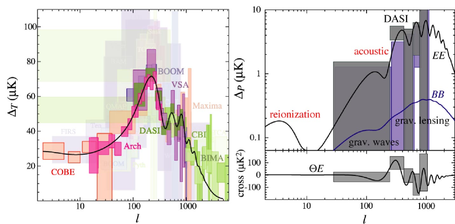
Figure 1: Power spectra data plotted as the rms contribution per logarithmic interval $[l(l+1)C_{l}/2\pi]^{1/2}$ with error boxes representing $1\sigma$ error bars and approximate multipole bandwidth. Overplotted is a scale-invariant, flat cosmological model with $\Omega_{m}=1/3$, $\Omega_{\Lambda}=2/3$, $h=0.7$, $\Omega_{b}h^{2}=0.02$, reionization redshift $z_{i}=7$, and an inflationary energy scale of $E_{i}=2.2\times 10^{16}$ GeV.

The primary observable is the two point correlation between fields $X,X^{\prime}\in\{\Theta,E,B\}$

$$\left<X_{lm}^{*}X_{l^{\prime}m^{\prime}}^{\prime}\right> =\delta_{ll^{\prime}}\delta_{mm^{\prime}}C_{l}^{XX^{\prime}}\,,$$ (3)

and are described by power spectra $C_{l}$ as long as the fields are statistically isotropic. If parity is also conserved then $B$ has no correlation with $\Theta$ or $E$. If in addition the fluctuations are Gaussian distributed, the power spectra contain all of the statistical information about the fields. The measurements of these power spectra to date are shown in Fig. 1.

3 Photon-Baryon Plasma

3.1 Cosmological Background

We begin with a brief review of the cosmological background and the parameters that govern it. The expansion of the universe is described by the scale factor $a(t)$, set to unity today, or equivalently the redshift $z(t)=a(t)^{-1}-1$, and by the current expansion rate, the Hubble constant $H_{0}=100h$ km sec^-1 Mpc^-1. The universe is flat (no spatial curvature) if the total density is equal to the critical density, $\rho_{c}=1.88h^{2}\times 10^{-29}$g cm^-3; it is open (negative curvature) if the density is less than this and closed (positive curvature) if greater. The mean densities of different components of the universe control $a(t)$ and are typically expressed today in units of the critical density $\Omega_{i}$, with an evolution $\rho_{i}\propto a^{-3(1+w_{i})}$, where $w_{i}=p_{i}/\rho_{i}$ with $p_{i}$ is the pressure. In particular the CMB photons have $w_{\gamma}=1/3$ and so $\rho_{\gamma}\propto a^{-4}$ or $T\propto a^{-1}$. The quantities $\Omega_{i}h^{2}$ are proportional to the physical density of the species today. We will be interested in the baryonic component $\Omega_{b}h^{2}$ and the total non-relativistic matter $\Omega_{m}h^{2}$, where the difference is made up of cold dark matter. We also allow for a dark energy component $\Omega_{e}$, with an equation of state parameter $w_{e}$ which for illustrative purposes we often take to be a cosmological constant ($\Omega_{\Lambda}$, $w_{\Lambda}=-1$) as consistent with indications from distant supernovae Rieetal98 ; Peretal99 . We represent the total density as $\Omega_{\rm tot}=\sum_{i}\Omega_{i}$ so that deviations from unity represent a spatially curved universe.

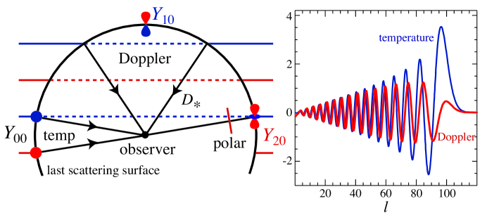
Figure 2: Geometric projection of sources at the last scattering surface into temperature and polarization anisotropy today. Left: the main sources of anisotropy are the effective local temperature which has a monopole structure ($Y_{00}$), the Doppler effect which has a dipole structure ($Y_{10}$) and the quadrupole source of polarization ($Y_{20}$) decomposed into plane waves. Right: the projection of the sources involves a coupling of the plane wave angular dependence or momenta with that of the source. A plane wave temperature inhomogeneity produces a sharp peak in the anisotropy at $l\approx kD_{*}(=100$ here) reflecting the structure of $j_{l}(kD_{*})$ shown; the Doppler effect does not produce peaks since the coupling involves $l\pm 1$ in the combination $j_{l}^{\prime}(kD_{*})$. The functions here are weighted by $2l+1$ to account for the number of modes.

3.2 Sources of Anisotropy

As the CMB cools due to the expansion, the photons eventually no longer have sufficient energy to overcome the binding energy of hydrogen $B=13.6$eV to keep the medium ionized. After this epoch, CMB photons propagate essentially unimpeded to the observer. This transition, called recombination, occurs relatively rapidly around $a_{*}\approx 10^{-3}$ at an energy scale of $\sim 1/3$ eV as can be seen by the equilibrium Saha equation

$${x_{e}^{2}\over 1-x_{e}} ={n_{e}n_{p}\over n_{H}n_{b}}={1\over n_{b}}\left({m_{e}T\over 2\pi}\right)^{3/2}e^{-B/T}$$

$$\approx 3\times 10^{15}\left({\Omega_{b}h^{2}\over 0.02}\right)^{-1}\left({B\over T}\right)^{3/2}e^{-B/T}\,,$$ (4)

where $x_{e}$ is the ionization fraction of hydrogen and we have neglected a small contribution from helium. The low $T/B$ of the transition is mainly due to the low baryon-photon ratio of the universe. It is sufficient that photons in the tail of the blackbody distribution be energetic enough to ionize hydrogen. In reality, recombination is slightly less rapid than implied by the Saha equation since processes which account for net recombination are not sufficiently rapid to maintain equilibrium toward the end of recombination Pee68 ; ZelKurSun69 (see SeaSasSco00 for refinements). Nonetheless the transition is sufficiently rapid that the photons in the CMB originate from a sharply defined surface or photosphere called the last scattering surface.

The properties of the plasma on this surface directly translate into the observable primary temperature and polarization anisotropy in the CMB. These properties are themselves governed by Thomson scattering of photons off of free electrons, which has a differential cross section of

$${d\sigma\over d\Omega}={3\over 8\pi}|\hat{\bf E}^{\prime}\cdot\hat{\bf E}|^{2}\sigma_{T}\,,$$ (5)

where $\sigma_{T}=8\pi\alpha^{2}/3m_{e}$ is the Thomson cross section, $\hat{\bf E}^{\prime}$ and $\hat{\bf E}$ denote the incoming and outgoing directions of the electric field or polarization vector. Summed over polarization and incoming angle, the comoving mean free path of a photon in the electrons is

$$\dot{\tau}^{-1} ={1\over n_{e}\sigma_{T}a}\approx 2.5\left(x_{e}{\Omega_{b}h^{2}\over 0.02}\right)^{-1}\left({a_{*}\over 10^{-3}}\right)^{2}{\rm Mpc}\,,$$ (6)

which is relatively small by cosmological standards. Overdots here and below represent derivatives with respect to conformal time. Electrons are coupled to baryons by Coulomb interactions and so on scales larger than $\dot{\tau}^{-1}$, the photon-baryon plasma can be considered a nearly perfect fluid PeeYu70 . In particular, rapid scattering keeps the photons isotropic in the baryon rest frame and so sets its dipole moment equal to the baryon velocity.

The tight coupling approximation implies that the CMB is described by relatively few quantities. There is the local temperature, or monopole, in space $\Theta_{00}({\bf x})$, the dipole $\Theta_{1m}({\bf x})$ and a residual but important quadrupole moment $\Theta_{2m}({\bf x})$ from the breakdown of tight coupling. In addition, the photons experience a gravitational redshift from gravitational potentials and gravitational waves. Modern CMB codes SelZal96 ; LewChaLas00 track the evolution of these sources BonEfs84 ; VitSil84 and construct the present day CMB temperature and polarization anisotropy spectrum by geometric projection.

As a simple example, let us consider the spatial temperature perturbation $\Theta({\bf x})\equiv\sqrt{4\pi}\Theta_{00}({\bf x})$, where the normalization convention reflects that of $Y_{lm}$, on a last scattering surface considered to be infinitely sharp at a comoving distance $D_{*}$ (see Fig. 2). In a flat universe, the spatial field may be represented by its Fourier harmonics

$$\Theta(\hat{\bf n}) =\int dD\Theta({\bf x})\delta(D-D_{*})$$

$$=\int{d^{3}k\over(2\pi)^{3}}\Theta({\bf k})e^{i{{\bf k}\cdot D_{*}\hat{\bf n}}}\,.$$ (7)

In an spatially curved universe, the plane waves must be replaced by the eigenfunctions of the Laplace operator to account for a change in the relationship between distance and angle that we discuss below. Also to achieve high precision in the predictions, the delta function must be replaced by the visibility function $\dot{\tau}e^{-\tau}$, the probability of a photon last scattering in a distance interval $dD$ to account for the finite duration of recombination.

Expanding the plane waves in spherical harmonics, we obtain

$$\Theta_{lm}=\int{d^{3}k\over(2\pi)^{3}}\Theta({\bf k})4\pi i^{l}j_{l}(kD_{*})Y_{lm}(\hat{\bf k})\,.$$ (8)

The power spectrum of the anisotropy contributions from the local temperature is then governed by that of the spatial temperature field at recombination

$$\langle\Theta^{*}({\bf k})\Theta({\bf k}^{\prime})\rangle\equiv(2\pi)^{3}\delta({\bf k}-{\bf k}^{\prime})P_{T}(k)\,,$$ (9)

such that

$$C_{l}^{\Theta\Theta} =4\pi\int{dk\over k}\,j_{l}^{2}(kD_{*}){k^{3}P_{T}(k)\over 2\pi^{2}}\,.$$ (10)

Note that the quantity $k^{3}P_{T}/2\pi^{2}$ is the contribution per log interval to the variance of the temperature $\sigma^{2}=\int d^{3}k/(2\pi)^{3}P_{T}$. For a slowly-varying log power, the integral in Eqn. (10) can be performed analytically

$${l(l+1)\over 2\pi}C_{l}^{\Theta\Theta} \equiv\left(\Delta_{T}^{2}\over T^{2}\right)\approx{k^{3}P_{T}(k)\over 2\pi^{2}}\Big{|}_{k=l/D_{*}}\,,$$ (11)

and so it is convenient to represent the anisotropy by the rms temperature contribution per log interval $\Delta_{T}$. It is also the contribution to the anisotropy variance per log interval in $l$ for $l\gg 1$. We also define the analogous quantities to describe the polarization fields ($\Delta_{P}$) and the temperature-polarization cross correlations ($l(l+1)C_{l}^{\Theta E}/2\pi$).

This behavior of the local temperature is representative of the other sources with a few important differences. In general, power from low order multipole moments $l=0,1,2$ in the CMB project into higher order anisotropy today by simple geometry BonEfs87 . The local temperature is an $l=0$ source. Note that the spherical Bessel function $j_{l}(x)$ peaks at $l\sim x$ (see Fig. 2 right) and so the translation in Eqn. (8) from power in real space to angular space is nearly one-to-one. Thus in Eqn. (11) one takes $kD_{*}\approx l$ with features in one preserved in the other. This corresponds to an edge-on ($\hat{\bf n}\perp{\bf k}$) projection of the wavelength of the fluctuation onto angle: $\theta=\lambda/D_{*}$.

Other sources of anisotropy have angular dependence on the last scattering surface which changes the relationship between $l$ and $k$. The dipole term provides an instructive example. It represents Doppler shifts in the temperature due to the motion of the photon-baryon plasma along the line of sight. For a curl free flow as expected cosmologically, there is no contribution to the Doppler effect for $\hat{\bf n}\perp{\bf k}$ and the peak structure is washed out. Mathematically, the Doppler effect contributes a dipole term $\hat{\bf n}\cdot{\bf k}\propto Y_{1m}$ which when coupled to the plane wave angular momentum $Y_{lm}$ leads to a recoupling of $j_{l\pm 1}$ to $j_{l}^{\prime}$ (see Fig. 2). Unlike $j_{l}$, $j_{l}^{\prime}$ has no peak structure leading to a one-to-many projection of $k$ onto $l$. Geometrically, well-defined features such as peaks in the anisotropy spectrum cannot come from the Doppler effect HuSug95a . All sources may be described in this framework of the addition of local angular momentum with plane wave orbital angular momentum with the net effect of modifying the mapping between $k$ and $l$ space HuWhi97c .

The local quadrupole plays a special role in that it is the fundamental source of linear polarization in the CMB as can be seen from the Thomson differential cross section of Eqn. (5). Heuristically, incoming radiation shakes an electron in the direction of its electric field vector $\hat{\bf E}^{\prime}$ causing it to radiate with an outgoing polarization parallel to that direction. However since the outgoing polarization $\hat{\bf E}$ must be orthogonal to the outgoing direction, incoming radiation that is polarized parallel to the outgoing direction cannot scatter, leaving only one polarization state. If the intensity were completely isotropic the missing polarization state is supplied by radiation incoming from the direction orthogonal to the original one. Only a quadrupole temperature anisotropy in the radiation generates a net linear polarization from Thomson scattering. In particular, the polarization is oriented along the cold axis of the quadrupole moment in the transverse plane. We shall see that the breakdown of tight coupling during recombination allows quadrupoles to be generated out of gradients in the fluid velocity and from gravitational redshifts associated with gravitational waves. For the former, since the quadrupole axis is aligned with the wavevector, the polarization generated is a pure $E$-mode (see Fig. 2). Gravitational waves generate both $E$ and $B$ modes KamKosSte97 ; ZalSel97 .

To understand the phenomenology of the anisotropy in the CMB temperature and polarization fields it is sufficient to understand the dynamics governing the local sources: the monopole, dipole and quadrupole of the CMB temperature field and their gravitational or metric fluctuation analogues.

3.3 Fluid Dynamics

The evolution of the anisotropy sources is governed by simple fluid dynamics. From the previous section, the critical variables are the monopole or temperature fluctuation $\Theta({\bf k})\equiv\sqrt{4\pi}\,\Theta_{00}({\bf k})$, the dipole or bulk velocity $v_{\gamma}({\bf k})=-i\sqrt{4\pi/3}\,\Theta_{10}({\bf k})$, and the quadrupole or anisotropic stress $\pi_{\gamma}({\bf k})=-(12/5)\sqrt{4\pi/5}\,\Theta_{20}({\bf k})$. We will hereafter drop the argument ${\bf k}$ with the understanding that the Fourier representation is always assumed. For convenience we have chosen the coordinate system so that ${\bf z}\parallel{\bf k}$ so that the plane waves are azimuthally symmetric and stimulate only the $m=0$ mode (see Fig. 2). Likewise we have suppressed the vector dependence of the bulk velocity by the same assumption ${\bf v}_{\gamma}=-iv_{\gamma}\hat{\bf k}$. The analogous quantities for the baryons are the density perturbation $\delta_{b}$ and bulk velocity $v_{b}$. For gravity, we choose a conformal Newtonian representation (see e.g. MaBer95 ) where the gravitational potential perturbations are defined by the Newtonian potential $\Psi$ (time-time metric fluctuation) and the curvature fluctuation $\Phi$ (space-space metric fluctuation $\approx-\Psi$).

Covariant conservation of energy and momentum requires that the photons and baryons satisfy separate continuity equations

$$\dot{\Theta}=-{k\over 3}v_{\gamma}-\dot{\Phi}\,,\qquad\dot{\delta}_{b}=-kv_{b}-3\dot{\Phi}\,,$$ (12)

and coupled Euler equations

$$\dot{v}_{\gamma} =k(\Theta+\Psi)-{k\over 6}\pi_{\gamma}-\dot{\tau}(v_{\gamma}-v_{b})\,,$$

$$\dot{v}_{b} =-{\dot{a}\over a}v_{b}+k\Psi+\dot{\tau}(v_{\gamma}-v_{b})/R\,,$$ (13)

where $R=(p_{b}+\rho_{b})/(p_{\gamma}+\rho_{\gamma})\approx 3\rho_{b}/4\rho_{\gamma}$ is the photon-baryon momentum density ratio. We have neglected a small correction to the anisotropic stress term in a curved universe.

The continuity equations represent particle number conservation. For the baryons, $\rho_{b}\propto n_{b}$. For the photons, $T\propto n_{\gamma}^{1/3}$, which explains the $1/3$ in the velocity divergence term. The $\dot{\Phi}$ terms come from the fact that $\Phi$ is a perturbation to the scale factor and so they are the perturbative analogues of the cosmological redshift and density dilution from the expansion. The Euler equations have similar interpretations. The expansion makes particle momenta decay as $a^{-1}$. The cosmological redshift of $T$ accounts for this effect in the photons. For the baryons, it becomes the expansion drag on $v_{b}$ ($\dot{a}/a$ term). Potential gradients $k\Psi$ generate potential flow. For the photons, stress gradients in the fluid, both isotropic ($k\delta p_{\gamma}/(p_{\gamma}+\rho_{\gamma})=k\Theta$) and anisotropic ($k\pi_{\gamma}$) counter infall. Thomson scattering exchanges momentum between the two fluids ($\dot{\tau}$ terms).

For scales much larger than the mean free path $\dot{\tau}^{-1}$, the Euler equation may be expanded to leading order in $k/\dot{\tau}$, such that the photons are isotropic in the baryon rest frame $v_{\gamma}=v_{b}$ and so the joint Euler equation becomes

$${d\over d\eta}[(1+R)v_{\gamma}]=k[\Theta+(1+R)\Psi]\,.$$ (14)

Combining this with the continuity equation leads to the oscillator equation (e.g. HuSug95a )

$${d\over d\eta}[(1+R)\dot{\Theta}]+{k^{2}\over 3}\Theta=-{k^{2}\over 3}(1+R)\Psi-{d\over d\eta}[(1+R)\dot{\Phi}]\,,$$ (15)

and a small residual anisotropic stress or quadrupole that tracks the evolution of the fluid velocity Kai83 ,

$$\pi_{\gamma}={32\over 15}{k\over\dot{\tau}}v_{\gamma}\,.$$ (16)

This dependence reflects the fact that a local quadrupole can arise from a gradient in the velocity field, for example as photons from two hot crests of a plane wave fluctuation meet at the trough in between (see Fig. 2 left), but is suppressed by scattering.

Equation (15) is the fundamental relation for acoustic oscillations. The change in the momentum of the photon-baryon fluid is determined by a competition between the pressure restoring and gravitational driving forces which causes the system to oscillate around its equilibrium. Note that the frequency of the oscillation

$$\omega^{2}={1\over 3(1+R)}k^{2}=c_{s}^{2}k^{2}\,,$$ (17)

where $c_{s}$ is the sound speed of the fluid.

Equation (16) is the fundamental relation for acoustic polarization. Its quadrupole source tracks the motion of the fluid. Polarization is generally small, at most $\sim$10% of the anisotropy itself, since it requires scattering for its generation but its quadrupole source is suppressed if the scattering is too rapid. Given the initial conditions and gravitational potentials, these equations predict the phenomenology of the acoustic oscillations in the temperature and polarization fields.

3.4 Initial Conditions

The simplest inflationary models make a set of definite predictions for the initial conditions of the acoustic oscillations and hence their successful observation provides strong support for the inflationary paradigm. Quantum fluctuations in the scalar field that drives inflation imprints a nearly spectrum of Gaussian curvature (potential) fluctuations $k^{3}P_{\Phi}/2\pi^{2}\propto k^{n-1}$ where $n\approx 1$ GutPi82 ; Haw82 ; BarSteTur83 on a spatially flat background metric. Gravitational infall into these initial potentials eventually generates all of the structure in the universe. Quantum fluctuations in the gravitational wave degrees of freedom also produce a nearly scale-invariant spectrum of fluctuations whose power depends on $E_{i}^{4}$ where $E_{i}$ is the energy scale of inflation RubSazVer82 ; FabPol83 .

A Newtonian gravitational potential $\Psi\approx-\Phi$ necessarily imparts an initial temperature perturbation since $\Psi$ represents a spatially varying time-time perturbation to the metric away from coordinates where the temperature is homogeneous. The perturbation is equivalent to a change in the scale factor since

$$a\propto t^{2\over 3(1+p/\rho)}\,,$$ (18)

which then produces a change in the temperature perturbation from the cosmological redshift $T\propto a^{-1}$ of

$$\Theta=-{2\over 3(1+p/\rho)}\Psi$$ (19)

or $-\Psi/2$ in the radiation dominated era Pea91 ; WhiHu97 . We call $\Theta+\Psi$ the effective temperature since it also accounts for the redshift a photon experiences when climbing out of a potential well, also known as the Sachs-Wolfe effect SacWol67 . In the matter dominated epoch, $\Theta+\Psi=\Psi/3$.

There are three important aspects of these results. First, inflation sets the temporal phase of all wavemodes by starting them all at the initial epoch. We shall see that this predicts a coherent set of peaks in the CMB spectrum with a definite phase. Cosmological defect models predict a more random distribution of acoustic phases which produces incoherent acoustic phenomena AlbCouFerMag96 ; Alletal97 ; SelPenTur97 . Defects can be now be ruled out as a primary mechanism for structure formation in the universe. More generally, without inflation or some other modification to the matter-radiation dominated universe, curvature perturbations cannot be generated outside the apparent horizon and so build up only by the causal motion of matter. This generally entails at least a delay in temporal phase of the oscillations which is not observed.

Secondly, since the power spectrum of the effective temperature is directly related to scale-invariant curvature fluctuations from inflation, Eqn. (11) implies the acoustic oscillations should also be approximately scale invariant in amplitude in the tight coupling regime. Observations are in excellent agreement with this fundamental prediction with tight constraints on the index $n=0.94^{+0.11}_{-0.04}$ (Bonetal02 , see also KnoChrSko01 ; WanTegZal02 ; Peretal02 ). We will therefore base the discussion of the acoustic phenomenology on models with nearly scale-invariant initial curvature fluctuations as predicted by inflation.

Finally, the scale-invariant gravitational wave background leads to a quadrupolar distortion in the CMB temperature field just like its effect on a ring of test masses. Because the quadrupole axes lie in the plane transverse to the wavevector, this quadrupole anisotropy leads to $B$-mode polarization as the tight coupling approximation breaks down. A measurement of $B$-modes from gravitational waves would determine the energy scale of inflation $E_{i}$ but its strong scaling with $E_{i}$ implies that it can only open a relatively small window between a few $10^{15}$ – few $10^{16}$ GeV for possible detection KnoSon02 .

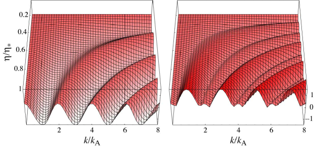
Figure 3: Temporal evolution of the effective temperature as a function of wavenumber predicted by the simplified model of Eqn. (23). Left: amplitude; right: rms fluctuation. All modes begin with the same phase and are frozen in at the same time $\eta=\eta_{*}$. The result is a harmonic series of extrema with a fundamental scale of $k_{A}=\pi/s_{*}$. Baryons, here shown with an $R=0.6(\eta/\eta_{*})^{2}$, displace the zero point of the oscillation and enhance the compressional troughs. In the rms, this leads to enhanced odd numbered peaks.

4 Acoustic Phenomenology

4.1 Acoustic Scale

It is instructive to first consider a simplified model where the universe is always matter-dominated in its expansion and the dynamical effects of the baryons are negligible. This amounts to holding $\Phi$ and $\Psi$ constant in the oscillator equation (15) and setting $R=0$. The solution for an initial curvature fluctuation is then simple

$$[\Theta+\Psi](k,\eta)={1\over 3}\Psi(k,0)\cos(ks)\,,\qquad v_{\gamma}(k,\eta)={\sqrt{3}\over 3}\Psi(k,0)\sin(ks)\,,$$ (20)

where $s=\int_{0}^{\eta}c_{s}d\eta^{\prime}$ is the distance sound can travel by $\eta$ or the sound horizon.

In the limit of scales large compared with the sound horizon $ks\ll 1$, the perturbation is frozen into its initial conditions. This is the gist of the statement that the large-scale anisotropy measured by COBE directly measure the initial conditions. On small scales, the amplitude of the Fourier modes exhibits temporal oscillations corresponding to compression and rarefaction of the plasma inside gravitational potential wells. All modes are frozen in at recombination $\eta_{*}$ (see Fig. 3 left). Modes that are caught at either maxima or minima of their oscillation at recombination correspond to peaks in the rms fluctuation or power (see Fig. 3 right). Given the solution in Eqn. (20), these modes are harmonics $k_{n}=nk_{A}$ of a fundamental acoustic scale $k_{A}=\pi/s_{*}$, where $n$ is an integer (see Figure 3a). From Eqn. (11), these become angular peaks in the anisotropy power with a characteristic angular scale of $l_{A}=k_{A}D_{*}$. The Doppler effect from the line-of-sight velocity has an rms $v_{\gamma}/\sqrt{3}$ and so contributes an equal amplitude fluctuation. It is $\pi/2$ out of phase with the temperature. This is because extrema represent turning points in the oscillation where the velocity vanishes. Nonetheless, because of the geometry of the projection (see Fig. 2), these oscillations do not contribute peaks in the angular power spectrum. We shall see that they do however predict the peaks in the polarization spectrum through Eqn. (16).

Under the flat, matter-dominated assumption the horizon distance scales as $\eta\propto a^{1/2}$. Thus $s_{*}\approx D_{*}/\sqrt{3000}$ and so $l_{A}\approx 200$. In a spatially curved universe, the distance used in the conversion from $k$ to $l$ no longer equals the comoving distance $D_{*}\neq\eta(a=1)-\eta_{*}$. Consider first a closed universe with radius of curvature $R=H_{0}^{-1}|\Omega_{\rm tot}-1|^{-1/2}$. Suppressing one spatial coordinate yields a 2-sphere geometry with the observer situated at the pole (see Fig. 4 left). Light travels on lines of longitude. A physical scale $\lambda$ at fixed latitude given by the polar angle $\theta$ subtends an angle $\alpha=\lambda/R\sin\theta$. For $\alpha\ll 1$, a Euclidean analysis would infer a distance $D=R\sin\theta$, even though the coordinate distance along the arc is $d=\theta R$; thus

$$D=R\sin(d/R)\,.$$ (21)

For open universes, simply replace $\sin$ with $\sinh$. The peak locations $l_{n}=nk_{A}D_{*}$ making them extremely sensitive to the spatial curvature (DorZelSun78, ; KamSpeSug94, ); measurements constrain the geometry to be close to flat, consistent with a radius of curvature that is larger than the observable universe. Since a flat universe is at the critcal density, local measurements of a low matter density indicate that there is a missing or “dark” component of the energy density, in good agreement with indications of an accelerating expansion from distant supernovae.

These simple scalings must be modified for the fact that the universe is not fully matter dominated at recombination, the fluid is not purely photon-dominated, and the expansion is dark energy dominated today. The main effect is from the radiation density which changes the expansion rate and so shifts the acoustic scale to higher multipoles. For a flat universe with $\Omega_{m}h^{2}\approx 0.15$, $l_{A}\approx 300$ which is a substantial shift. The baryons lower the sound speed and so have a similar but smaller effect. The dark energy also provides a smaller effect through a decrease in the distance to recombination $D_{*}$ and hence a lowering of $l_{A}$, with an increase in $\Omega_{e}$ or $w$. The sensitivity of the acoustic scale to cosmological parameters is approximately (see also Fig. 5)

$${\Delta l_{A}\over l_{A}}\approx-1.1{\Delta\Omega_{\rm tot}\over\Omega_{\rm tot}}-0.24{\Delta\Omega_{m}h^{2}\over\Omega_{m}h^{2}}-0.17{\Delta\Omega_{e}\over\Omega_{e}}-0.11\Delta w_{e}+0.07{\Delta\Omega_{b}h^{2}\over\Omega_{b}h^{2}}\,,$$ (22)

around a model of $\Omega_{\rm tot}=1$, $\Omega_{m}h^{2}=0.15$$,\Omega_{e}=0.65$, $w_{e}=-1$ and $\Omega_{b}h^{2}=0.02$ HuFukZalTeg00 . A joint analysis of the data yields $l_{A}=304\pm 4$ KnoChrSko01 and with these errors, the uncertainty in the cosmological interpretation in the dark energy and curvature domain is already dominated by uncertainty in $\Omega_{m}h^{2}$ not peak measurement error (see Fig. 4 right). Fortunately as we shall see, this parameter can be internally determined from the CMB and serves as an example where future increased precision will have important implications for a quantity of fundamental interest, the dark energy.

Finally, there is a separate effect on the first peak. We shall see that the decay of the gravitational potential in a radiation dominated universe generates anisotropy from gravitational redshifts after last scattering, filling in the rise to the first peak and shifting its location downwards off of the harmonic series to $l_{1}\approx 3l_{A}/4$, placing $l_{1}\approx 220$ in agreement with the observed location Benetal02 .

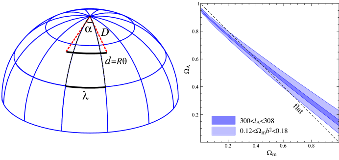
Figure 4: The acoustic scale. Left: geometrical effect in a closed universe. Objects in a closed universe are further than they appear ($D<d$). Consequently the measured angular scale of the peaks is extremely sensitive to the curvature, once the physical scale has been set by the acoustic physics. Right: translation of a constraint on the peak scale $300<l_{A}<308$ KnoChrSko01 (68% CL) onto the cosmological parameters $\Omega_{m}$ and $\Omega_{\Lambda}$ with all other parameters fixed versus constraints with uncertainties in the physical matter density $\Omega_{m}h^{2}$ from CMB determinations Bonetal02 folded in. Uncertainties in this plane are no longer dominated by peak location measurement errors.

4.2 Baryon loading

Baryons add to the mass of the photon-baryon plasma without adding to the pressure. An examination of Eqn. (15) shows that their effect comes solely through the baryon-photon momentum density ratio $R\approx 0.6(\Omega_{b}h^{2}/0.02)(a/10^{-3})$. It is instructive to look at the solution to the oscillator equation (20) in the approximation that $R$ is constant. Again under the assumption of a matter-dominated universe, the solution is that of a simple harmonic oscillator in a constant gravitational field but with an increased mass term

$$[\Theta+\Psi](k,\eta_{*}) =[\Theta+(1+R)\Psi](k,0)\cos(ks)$$

$$=[1+3R]{1\over 3}\Psi(0)\cos(ks)-R\Psi(0)\,,$$ (23)

where the sound speed entering into the sound horizon calculation is reduced since $c_{s}^{2}=1/3(1+R)$. Aside from this reduction, baryons have two distinguishing effects: they enhance the amplitude of the oscillations by $1+3R$ fractionally and shift the zero point of the oscillation by $-R\Psi$. The latter modulates the amplitude of neighboring peaks: odd numbered peaks will be enhanced over the zero-baryon case by $1+6R$; even numbered peaks remain the same (see Fig. 3, right). Physically, the baryon mass enhances compression inside gravitational potential wells.

These qualitative results remain true in the presence of the real time-variable $R$. Measurement of these baryonic signatures currently limits $\Omega_{b}h^{2}=0.022^{+0.004}_{-0.002}$ Bonetal02 . This value is strikingly consistent with inferences of the baryon density from big bang nucleosynthesis. Consequently there have been no significant changes in the baryon-photon ratio from an energy scale of an MeV to an eV in the expansion history of the universe.

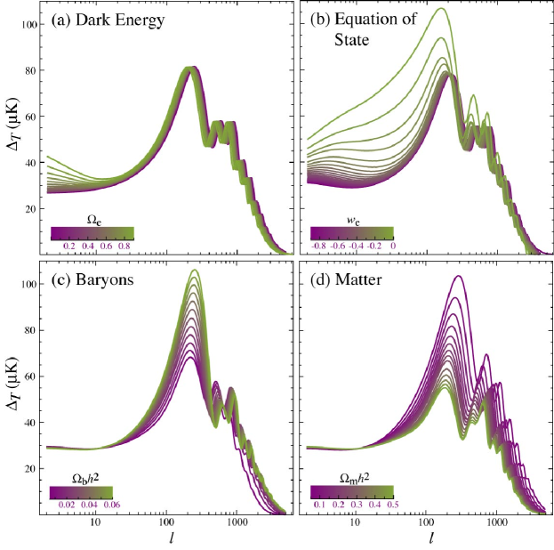
Figure 5: Sensitivity of the temperature power spectrum to four fundamental cosmological parameters: the energy density of the dark energy today $\Omega_{e}$ in units of the critical density, the equation of state parameter of the dark energy $w_{e}$, the physical baryon density $\Omega_{b}h^{2}$ and the physical matter density $\Omega_{m}h^{2}$. All are varied around a fiducial flat model of $\Omega_{e}=0.65$, $w_{e}=-1$, $\Omega_{b}h^{2}=0.02$ and $\Omega_{m}h^{2}=0.15$ with $n=1$.

4.3 Dark Matter and Radiation

The matter-to-radiation ratio scales as $\rho_{m}/\rho_{r}\approx 3.6(\Omega_{m}h^{2}/0.15)(a/10^{-3})$ and so the universe is only barely matter-dominated at last scattering. Moreover fluctuations corresponding to the higher peaks entered the sound horizon at an earlier time, during radiation domination. As we have seen, including the radiation changes the expansion rate of the universe and hence the physical scale of the sound horizon at recombination. Fortunately, radiation has the more unique effect of driving the acoustic oscillations by making the gravitational force evolve with time (HuSug95a, ).

The exact evolution of the potentials is determined by the relativistic Poisson equation. Its qualitative content is clear: since the background density is decreasing with time, the density fluctuations must grow unimpeded by pressure to maintain constant potentials. In particular, in the radiation dominated era once pressure begins to fight gravity at the first compressional extrema of the oscillation, the Newtonian gravitational potential and spatial curvature must decay.

This decay actually drives the oscillations: it is timed to leave the fluid maximally compressed with no gravitational potential to fight as it turns around. The net effect is doubled since the redshifting from the spatial metric fluctuation $\Phi$ also goes away at the same time. When the universe becomes matter dominated the gravitational potential is no longer determined by photon-baryon density perturbations but by the pressureless dark matter. Therefore, the amplitudes of the acoustic peaks increase as the matter-to-radiation ratio decreases (Sel94, ; HuSug95a, ). The net result is that across the horizon scale at matter-radiation equality the acoustic amplitude increases by a factor of

$${2\Psi-\frac{1}{3}\Psi\over\frac{1}{3}\Psi}=5$$ (24)

for a pure photon and dark matter universe, and a factor of 4 when including the effect of neutrinos and baryons HuSug96 (see also Fig. 6). By eliminating gravitational potentials, radiation also eliminates the alternating peak heights from baryon loading (see Fig. 5). The observed high third peak (see Fig. 1) is a good indication that matter dominates the energy density at recombination. Finally, the effect of the decaying potential after recombination leads to so-called integrated Sachs Wolfe contributions to the temperature fluctuations through the continuity equation (12) and shifts the first acoustic peak downwards off of the acoustic series HuSug95a .

Observations of these matter-radiation phenomena (see Fig. 5) currently constrain the total matter density to be $\Omega_{m}h^{2}=0.15\pm 0.03$ Bonetal02 and are crucial in internally resolving ambiguities in the interpretation of the peak scale. Since this number greatly exceeds the measured baryon density, these observations are also the first empirical indication that the dark matter exists at high redshift.

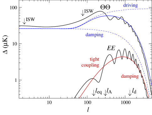
Figure 6: Phenomenological contributions to the anisotropy form. Radiation drives the amplitude of the acoustic oscillations up across the multipole scale subtended by the horizon at matter radiation equality $l_{\rm eq}$ and down across the damping scale $l_{D}$. Functional forms for these envelopes are taken from HuWhi97a . The ISW effect pushes $l_{1}<l_{A}$ due to the radiation and raises the large angle anisotropy due to the dark energy. The polarization scales as $l/l_{D}$ for $l<l_{D}$ due to the tight-coupling suppression of its quadrupole source and is also damped below $l_{D}$.

4.4 Damping

The photon-baryon fluid has slight imperfections corresponding to shear viscosity $\pi_{\gamma}$ and heat conduction $(v_{b}-v_{\gamma})$ in the Euler equation (13) Sil68 ; Wei71 . These imperfections damp acoustic oscillations. These are both associated with the diffusion of the photons which is especially important during recombination when the mean free path of the photons rises dramatically. As we have seen the viscosity $\pi_{\gamma}\sim kv_{\gamma}/\dot{\tau}$. With the continuity equation $kv_{\gamma}\approx-3\dot{\Theta}$, this leads to a $\dot{\Theta}$ damping term in the oscillator equation. The heat conduction term can be shown to have a similar effect by expanding the Euler equations in $k/\dot{\tau}$. An examination of the resulting damped oscillator equation shows that diffusion suppresses the oscillation amplitude by a factor of order $e^{-k^{2}\eta/\dot{\tau}}$. The damping scale $k_{\rm d}$ is thus of order $\sqrt{\dot{\tau}/\eta}$, corresponding to the geometric mean of the horizon and the mean free path. Detailed numerical integration of the equations of motion are required to track the rapid growth of the mean free path and damping length through recombination itself. These calculations show that the damping scale is of order $k_{\rm d}s_{*}\approx 10$ leading to a substantial suppression of the oscillations beyond the third peak (see Fig. 6). Observations of the damping phenomena provide a check on the fundamental assumptions underlying the interpretation of the acoustic peaks. With $\Omega_{b}h^{2}$ and $\Omega_{m}h^{2}$ and the acoustic scale $l_{A}$ fixed by the first few peaks, the damping scale is uniquely predicted given the atomic physics of recombination. Any change in recombination, for example due to a variation in the fine structure constant, will be revealed as a discrepancy in the predictions. Likewise, any misinterpretation of $l_{A}$ due to say initial conditions that were not purely curvature fluctuations resulting in a phase shift in the peaks would also show up as a discrepancy. The data in the damping tail to date are beautifully consistent with the predictions of the model (see Fig. 1).

4.5 Polarization

The dissipation of the acoustic oscillations leaves a signature in the polarization of the CMB in its wake. Recall that the observed polarization is a projection of the local quadrupole temperature anisotropy at last scattering. The fact that the polarization source is the quadrupole explains the shape and height of the polarization spectra in Fig. 1. Since the quadrupole is of order $kv_{\gamma}/\dot{\tau}\sim(k/k_{\rm d})(k_{d}\eta_{*})^{-1}v_{\gamma}$ (see Eqn. 16), the polarization spectrum rises as $l/l_{D}$ to peak at the damping scale with an amplitude of about 10% of the temperature fluctuations before falling due to the elimination of the acoustic source itself due to damping. Since $v_{\gamma}$ is out of phase with the temperature, the polarization peaks are also out of phase with the temperature peaks. Furthermore, the phase relation also tells us that the polarization is correlated with the temperature perturbations. The correlation power $C_{l}^{\Theta E}$ being the product of the two, exhibits oscillations at twice the acoustic frequency. As in the case of the damping, the predicting the precise value requires numerical work (BonEfs87, ) since $\dot{\tau}$ changes so rapidly near recombination. Nonetheless the detailed predictions shown in Fig. 6 bear these qualitative features.

The acoustic polarization and cross correlation has recently been detected by the DASI experiment Kovetal02 . Like the damping scale, the acoustic polarization spectrum is uniquely predicted from the temperature spectrum once $\Omega_{b}h^{2}$, $\Omega_{m}h^{2}$ are specified. Polarization thus represents a sharp test on the assumptions of the recombination physics and power law curvature fluctuations in the initial conditions used in interpreting the temperature peaks.

These acoustic peaks in the polarization appear exclusively in the $EE$ power spectrum due to the azimuthal symmetry of the plane wave fluctuations. During the break down of tight coupling that occurs at last scattering, any gravitational waves present will also imprint a local quadrupole anisotropy to the photons and hence a linear polarization to the CMB Pol85 . These contribute to the $BB$ power and their detection would provide invaluable information on the origin of the fluctuations (see e.g. SteTur01 ). Specifically, in simple inflationary models their amplitude gives the energy scale of inflation. The gravitational wave amplitude $h$ oscillates and decays once inside the horizon, so the associated polarization source scales as $\dot{h}/\dot{\tau}$ and so peaks at the $l\approx 100$ horizon scale and not the damping scale at recombination (see Fig. 1). This provides a useful scale separation of the various polarization effects.

5 Secondary Anisotropy

5.1 Gravitational Secondaries

As the photons travel from the last scattering surface to the observer, they traverse the large-scale structure of the universe leaving subtle imprints in the temperature and polarization fields.

There are two main gravitational effects. Intervening mass along the line of sight gravitationally lenses the CMB photon trajectories BlaSch87 and hence distorts both the temperature and polarization anisotropy fields. The photons are deflected according to the angular gradient of the potential projected along the line of sight,

$$\phi(\hat{\bf n})=2\int_{\eta_{*}}^{\eta_{a=1}}d\eta\,{(D_{*}-D)\over D\,D_{*}}\Phi(D\hat{\bf n},\eta)\,.$$ (25)

Because surface brightness is conserved in lensing, the deflection simply remaps the observed fields as

$$X(\hat{\bf n}) \rightarrow X(\hat{\bf n}+\nabla\phi)\,,$$ (26)

where $X\in\{\Theta$, $Q$, $U\}$. The typical deflection angle is of order a few arcminutes but the lines of sight are coherently deflected across scales of a few degrees. Since the coherence scale of the acoustic features is larger than the deflection angle, the lensing effect can be calculated by Taylor expanding Eqn. (26) (e.g. Hu00b ). The result is a product of fields so that in harmonic space the modes are coupled to each other across a range $\Delta l\approx 60$ set by the coherence of the deflection. Heuristically, lensing distorts the hot and cold spots formed by the acoustic oscillations and hence the mapping of $k$ to $l$.

In the temperature power spectrum, this mode coupling smooths the acoustic peaks slightly Sel96b . For the polarization, the remapping not only smooths the $EE$-peaks but actually generates $B$-mode polarization ZalSel98 . Remapping by the lenses preserves the orientation of the polarization but warps its spatial distribution and hence does not preserve the symmetry of the original $E$-mode. Gravitational lensing represents a fundamental obstacle to detection of low amplitude gravitational waves from inflation.

Because the lensed CMB distribution is not linear in the fluctuations, higher order statistics are promising probes of lensing effects (Ber97, ; Ber98, ; ZalSel99, ; Zal00, ). In particular, the coupling of multipoles separated by $\Delta l<60$ can be used to construct a minimum variance estimator of the deflection potential $\phi(\hat{\bf n})$ out of pairs of moments Hu01b . These quadratic estimators are close in performance to the optimal but more complicated maximum likelihood estimator HirSel02 . Since small-scale polarization anisotropy is otherwise free of cosmological $B$-modes, most of the signal-to-noise in the reconstruction lies in the pairing of $E$-modes to neighboring lensing-generated $B$-modes HuOka02 . This correlation can in principle be used to map the deflection potential down to the $10^{\prime}$ scale. This mapping can in turn be used to measure the growth of structure from $z_{*}=10^{3}$ Hu01c and hence the properties of the dark matter, including any component from massive neutrinos. It can also be used to remove much of the contamination to the gravitational wave $B$-modes and bring the detection threshold for the energy scale of inflation down to a $E_{i}\approx{\rm few\,}10^{15}$ GeV KnoSon02 .

Gravitational potentials can also change the temperature anisotropy through gravitational redshifts. Density perturbations cease to grow once the dark energy dominates the expansion. As in the case of the matter-radiation transition, the gravitational potentials must then decay. The evolution of the gravitational potential under a smooth component of dark energy is given by

$$\frac{d^{2}\Phi}{d\ln a^{2}}+\left[\frac{5}{2}-\frac{3}{2}w_{e}(a)\Omega_{e}(a)\right]\frac{d\Phi}{d\ln a}+\frac{3}{2}[1-w_{e}(a)]\Omega_{e}(a)\Phi=0\,.$$ (27)

With the appropriate replacements, this equation also applies to smooth components of dark matter, e.g. a light neutrino. A scalar field candidate for dark energy is smooth out to the horizon scale at any given time CalDavSte98 .

As we have seen, a decay in the gravitational potential causes an effective heating of the photons in a gravitational well. Like the matter-radiation analogue, it is intrinsically a large effect since the net change due to the decay is $5$ times the Sachs-Wolfe effect of $\Psi/3$. However since the opposite effect occurs in underdense regions, the contributions are canceled as photons traverse many crests and troughs of the potential perturbation during the matter-dark energy transition. The effect, called the (late-time) integrated Sachs-Wolfe (ISW) effect SacWol67 ; KofSta85 , then appears only at large scales or low multipoles (see Fig. 6).

The ISW effect is the most direct signature of the dark energy available in the CMB and is very sensitive to its equation of state and clustering properties if it deviates far from a cosmological constant ($w_{e}>-1/2$, see Fig. 5), unfortunately given the large-scale nature of the effect, the limited number of samples of the low order multipoles, or “cosmic variance”, prevents a precise determination from the power spectrum. A promising technique is to isolate the ISW effect through its cross correlation with reconstructed lensing maps from the CMB (GolSpe99, ; ZalSel99, ; Hu01c, ).

5.2 Scattering Secondaries

The universe is observed to be ionized out to $z\approx 6$ and is thought to have undergone reionization sometime between between $7\leq z\mathrel{\hbox to0.0pt{\lower 3.0pt\hbox{$\mathchar 536\relax$}\hss}\raise 2.0pt\hbox{$\mathchar 316\relax$}}30$ (see BarLoe01 for a review). Consequently a minimum of a few percent of the photons have rescattered since recombination (see Eqn. 6). The main effect from rescattering of the photons during reionization is a uniform suppression of the peaks by $e^{-\tau}$ as anisotropy is destroyed by the randomization of directions in scattering. Since this can be confused with a change in the initial amplitude of fluctuations, it is important to resolve this ambiguity for the study of initial fluctuations and the growth rate of fluctuations, which itself probes the properties of the dark energy and dark matter through Eqn. (27). Reionization is interesting in its own right since it can us about the sources of ionizing radiation from the first astrophysical objects formed in the universe.

The most promising means of isolating the reionization effect through the CMB is from the generation of large scale polarization during recombination. The rescattered radiation becomes polarized since temperature inhomogeneities become anisotropies by projection (see Eqn. 8), passing through quadrupole anisotropy when the perturbations are on the horizon scale at any given time ($kD_{*}\approx k\eta\approx l=2$). The result is a peak in the $E$-mode power spectrum shown in Fig. 1. In a perfect, foreground-free world, even the minimal signal is within reach of the MAP MAP and Planck Planck satellites and can be used to isolate the reionization epoch (HogKaiRes82, ; Kapetal02, ).

The dissipation of the acoustic oscillations at small scales also provides a window through which to see subtler effects. The main contribution beyond the damping tail comes from the rescattering of the CMB off of hot electrons in clusters of galaxies, called the Sunyaev-Zeldovich effect SunZel72 . Inverse Compton scattering represents a net transfer of energy between the hot electron gas and the cooler CMB. It leaves a spectral distortion in the CMB where photons on the Rayleigh-Jeans side are transferred to the Wien tail. The effect in individual clusters is now routinely measured and is an important means of studying the physics of clusters and the dark energy CarHolRee02 . The effect of unresolved high redshift clusters may have already been detected in the CMB by the CBI and BIMA experiments, albeit at an amplitude that is somewhat higher than expected Bonetal02 ; KomSel02 . Confirmation of the nature of this small scale excess will require measurements at multiple frequencies to test its inverse Compton nature.

There are a host of smaller effects due to Doppler shifts of the moving ionized gas (see e.g. HuDod02 ). These present a significant challenge to detect and interpret and are beyond the scope of this review.

6 Discussion

The tremendous experimental progress in CMB anisotropy studies over the last few years has helped establish a standard paradigm for cosmology at intermediate epochs but has simultaneously raised questions about the physics at the two opposite ends of time. Simple inflationary models of the early universe have so far passed the test of the acoustic peaks. They predict the near scale-invariant initial curvature fluctuations in a spatially flat background that have now been observed. Moreover, spatial flatness appears to be maintained today by a mysterious form of missing or dark energy.

The first step into the future will come with the release of data from the MAP satellite in early 2003 which in the full course of the mission will provide the definitive measurement of temperature anisotropy across the whole sky down to a quarter of a degree. The MAP satellite will test the spectrum of initial conditions beyond the simple constraints on the power law index which can be extracted today (e.g. WanSpeStr99 ; TegZal02 ). These advances will come with the increased precision in the temperature measurements and determination of the acoustic peaks in the polarization and cross correlation. Measurement of the polarization peaks will not only eventually double the amount of statistical information that can be extracted from the CMB but can also provide a sharp distinction between small changes in the dynamics of the plasma, which affect temperature and polarization differently, and small deviations from scale invariance of in the initial conditions (e.g. EasGreKinShi02 ), which affect the two alike. Studies of the Gaussianity of the acoustic fluctuations will also provide a strong test of the inflationary model. The increased precision on the matter-radiation ratio will sharpen considerably the constraints on the dark energy. MAP should also be able to detect or place limits on the amount of reionization in the universe through a large angle bump in the polarization and hence remove a central ambiguity for dark energy and dark matter studies from the peaks.

The next generation of experiments dedicated to fine-scale, secondary structure in the anisotropy will enable new tests of the dark energy from structures in the universe such as galaxy clusters. They will also provide a new handle on reionization through the Doppler shift of CMB photons off of moving structures.

Further down the road lies the milestone of the gravitational lensing of the peaks. Detection will not only require more sensitive instruments and higher angular resolution but also subtraction of galactic and extragalactic foreground contaminants TegEisHudeO00 ; PruSetBou00 ; Bacetal02 . In principle higher order statistics can be used to reconstruct the potential field in projection with a large gains in sensitivity available if the $B$-modes from lensing can not only be detected but accurately mapped HuOka02 . From this reconstruction the dark matter and dark energy dependent growth of structure can be measured. For example gravitational lensing can enable tests of the scalar-field hypothesis for the nature of the dark energy through cross-correlation with the integrated Sachs-Wolfe effect Hu01c .

The ultimate future milestone for the CMB is the detection of gravitational waves from inflation through $B$-mode polarization. Detection would represent strong evidence for the inflationary model and pin down its energy scale. The window of detectability can be extended to energy scales above a few $10^{15}$ GeV but only if the $B$-modes from gravitational lensing are removed from a direct reconstruction.

These future milestones will require much experimental effort to achieve and much theoretical effort to interpret. Nevertheless they provide the hope that the next decade of studies of CMB temperature and polarization anisotropy will be as fruitful as the last.

References

- (1)
- (2) W. Hu, S. Dodelson, Ann. Rev. Astron. Astrophys. 40 (2002), 171.
- (3) M. White, J. Cohn, Am. J. Phys. 70 (2002), 106.
- (4) M. Bersanelli, D. Maino, A. Mennella, Nuovo Cimento in press (2002), astro-ph/0209215.
- (5) G.F. Smoot, et al. Astrophys. J Lett. 396 (1992), L1.
- (6) R.K. Sachs, A.M. Wolfe, Astrophys. J 147 (1967), 73.
- (7) J.R. Bond, A.H. Jaffe, L. Knox, Astrophys. J 533 (2000), 19.
- (8) A.D. Miller, et al. Astrophys. J Lett. 524 (1999), L1.
- (9) P. de Bernardis, et al. Nature 404 (2000), 955.
- (10) S. Hanany, et al. Astrophys. J Lett. 545 (2000), 5.
- (11) P.J.E. Peebles, J.T. Yu, Astrophys. J 162 (1970), 815.
- (12) A.G. Doroshkevich, Y.B. Zel’dovich, R.A. Sunyaev, Sov. Astron. 22 (1978), 523.
- (13) A. Benoit, et al. Astron. Astrophys. submitted (2002), astro-ph/0210305.
- (14) A. Albrecht, D. Coulson, P. Ferreira, J. Magueijo, Phys. Rev. Lett. 76 (1996), 1413.
- (15) B. Allen, R.R. Caldwell, S. Dodelson, L. Knox, E.P.S. Shellard, Phys. Rev. Lett. 79 (1997), 2624.
- (16) U. Seljak, U. Pen, N. Turok, Phys. Rev. Lett. 79 (1997), 1615.
- (17) A.G. Riess, et al. Astron. J 116 (1998), 1009.
- (18) S. Perlmutter, et al. Astrophys. J 517 (1999), 565.
- (19) N.W. Halverson, et al. Astrophys. J 568 (2002), 38.
- (20) P. de Bernardis, et al. Astrophys. J 564 (2002), 559.
- (21) P.F. Scott, et al. Mon. Not. R. Ast. Soc. (2002), astro-ph/0205380.
- (22) D.N. Schramm, M.S. Turner, Rev. Mod. Phys. 70 (1998), 303.
- (23) T.J. Pearson, et al. Astrophys. J submitted (2002), astro-ph/0205388.
- (24) B.G. Keating, et al. Astrophys. J Lett. 560 (2001), L1.
- (25) M. Hedman, et al. Astrophys. J 573 (2002), 73.
- (26) J. Kovac, et al. Astrophys. J submitted (2002), astro-ph/0209478.
- (27) P.J. Steinhardt, N. Turok, Phys. Rev. D 65 (2002), 126003.
- (28) B.S. Mason, et al. Astrophys. J submitted (2002), astro-ph/0205384.
- (29) K.S. Dawson, et al. Astrophys. J submitted (2002), astro-ph/0206012.
- (30) D.J. Fixsen, et al. Astrophys. J 473 (1996), 576.
- (31) J.R. Bond, G. Efstathiou, Mon. Not. R. Ast. Soc. 226 (1987), 655.
- (32) A. Kosowsky, Ann. Phys. 246 (1996), 49.
- (33) M. Kamionkowski, A. Kosowsky, A. Stebbins, Phys. Rev. D 55 (1997), 7368.
- (34) M. Zaldarriaga, U. Seljak, Phys. Rev. D 55 (1997), 1830.
- (35) E. Newman, R. Penrose, J. Math Phys. 7 (1966), 863.
- (36) J.N. Goldberg, et al. J. Math Phys. 7 (1966), 863.
- (37) U. Seljak, Astrophys. J 482 (1997), 6.
- (38) P.J.E. Peebles, Astrophys. J 153 (1968), 1.
- (39) Y. Zel’dovich, V. Kurt, R. Sunyaev, Sov. Phys.–JETP 28 (1969), 146.
- (40) S. Seager, D.D. Sasselov, D. Scott, ApJS 128 (2000), 407.
- (41) U. Seljak, M. Zaldarriaga, Astrophys. J 469 (1996), 437.
- (42) A. Lewis, A. Challinor, A. Lasenby, Astrophys. J 538 (2000), 473.
- (43) J.R. Bond, G. Efstathiou, Astrophys. J 285 (1984), 45.
- (44) N. Vittorio, J. Silk, Astrophys. J 285 (1984), L39.
- (45) W. Hu, N. Sugiyama, Astrophys. J 444 (1995), 489.
- (46) W. Hu, M. White, Phys. Rev. D 56 (1997), 596.
- (47) C.P. Ma, E. Bertschinger, Astrophys. J 455 (1995), 7.
- (48) N. Kaiser, Mon. Not. R. Ast. Soc. 202 (1983), 1169.
- (49) A.H. Guth, S.Y. Pi, Phys. Rev. Lett. 49 (1982), 1110.
- (50) S.W. Hawking, Phys. Lett. B 115 (1982), 295.
- (51) J.M. Bardeen, P.J. Steinhardt, M.S. Turner, Phys. Rev. D 28 (1983), 679.
- (52) V.A. Rubakov, M.V. Sazhin, A.V. Veryaskin, Phys. Lett. B115 (1982), 189.
- (53) R. Fabbri, M.D. Pollock, Phys. Lett B125 (1983), 445.
- (54) J. Peacock, Mon. Not. R. Ast. Soc. 253 (1991), 1P.
- (55) M. White, W. Hu, Astron. Astrophys. 321 (1997), 8.
- (56) J.R. Bond, et al. Theoretical Physics, MRST 2002 (2002), astro-ph/0210007.
- (57) L. Knox, N. Christensen, C. Skordis, Astrophys. J Lett. 563 (2001), 95.
- (58) X. Wang, M. Tegmark, M. Zaldarriaga, Phys. Rev. D 65 (2002), 123001.
- (59) W.J. Percival, et al. Mon. Not. R. Ast. Soc. in press (2002), astro-ph/0206256.
- (60) L. Knox, Y.S. Song, Phys. Rev. Lett. 89 (2002), 011303.
- (61) M. Kamionkowski, D.N. Spergel, N. Sugiyama, Astrophys. J 426 (1994), L57.
- (62) W. Hu, M. Fukugita, M. Zaldarriaga, M. Tegmark, Astrophys. J 549 (2001), 669.
- (63) U. Seljak, Astrophys. J 435 (1994), L87.
- (64) W. Hu, N. Sugiyama, Astrophys. J 471 (1996), 542.
- (65) J. Silk, Astrophys. J 151 (1968), 459.
- (66) S. Weinberg, Astrophys. J 168 (1971), 175.
- (67) W. Hu, M. White, Astrophys. J 479 (1997), 568.
- (68) A. Polnarev, Sov. Astron. 29 (1985), 607.
- (69) A. Blanchard, J. Schneider, Astron. Astrophys. 184 (1987), 1.
- (70) W. Hu, Phys. Rev. D 62 (2000), 043007.
- (71) U. Seljak, Astrophys. J 463 (1996), 1.
- (72) M. Zaldarriaga, U. Seljak, Phys. Rev. D 58 (1998), 023003.
- (73) F. Bernardeau, Astron. Astrophys. 324 (1997), 15.
- (74) F. Bernardeau, Astron. Astrophys. 338 (1998), 375.
- (75) M. Zaldarriaga, Phys. Rev. D 62 (2000), 063510.
- (76) W. Hu, Astrophys. J Lett. 557 (2001), L79.
- (77) C.M. Hirata, U. Seljak, Phys. Rev. D (2002), astro-ph/0209489.
- (78) W. Hu, T. Okamoto, Astrophys. J 574 (2002), 566.
- (79) W. Hu, Phys. Rev. D 65 (2002), 023003.
- (80) R.R. Caldwell, R. Dave, P.J. Steinhardt, Phys. Rev. Lett. 80 (1998), 1582.
- (81) L.A. Kofman, A.A. Starobinskii, Sov. Astron. 11 (1985), 27.
- (82) D.M. Goldberg, D.N. Spergel, Phys. Rev. D 59 (1999), 103002.
- (83) M. Zaldarriaga, U. Seljak, Phys. Rev. D 59 (1999), 123507.
- (84) R. Barkana, A. Loeb, Ann. Rev. Astron. Astrophys. 39 (2001), 19.
- (85) http://map.nasa.gsfc.gov
- (86) http://astro.estec.esa.nl/Planck
- (87) C.J. Hogan, N. Kaiser, M.J. Rees, Phil. Trans. R. Soc. A307 (1982), 97.
- (88) M. Kaplinghat, et al. Astrophys. J submitted (2002), astro-ph/0207591.
- (89) R. Sunyaev, Y. Zel’dovich, Comm. Astrophys. Sp. Phys 4 (1972), 173.
- (90) J.E. Carlstrom, G.P. Holder, E.D. Reese, Ann. Rev. Astron. Astrophys. 40 (2002), 643.
- (91) J.R. Bond, et al. Astrophys. J submitted (2002), astro-ph/0205386.
- (92) E. Komatsu, U. Seljak, Mon. Not. R. Ast. Soc. submitted (2002), astro-ph/0205468.
- (93) Y. Wang, D.N. Spergel, M.A. Strauss, Astrophys. J 510 (1999), 20.
- (94) M. Tegmark, M. Zaldarriaga, Phys. Rev. D in press (2002), astro-ph/0207047.
- (95) R. Easther, B.R. Greene, W.H. Kinney, G. Shiu, Phys. Rev. D 66 (2002), 023518.
- (96) M. Tegmark, D.J. Eisenstein, W. Hu, A. de Oliviera Costa, Astrophys. J 530 (2000), 133.
- (97) S. Prunet, S.K. Sethi, F.R. Bouchet, Mon. Not. R. Ast. Soc. 314 (2000), 348.
- (98) C. Baccigalupi, et al. Mon. Not. R. Ast. Soc. submitted (2002), astro-ph/0209591.