The Structure of Stellar Coronae in Active Binary Systems

Abstract

A survey of 28 stars (22 active binary systems, plus 6 single stars or wide binaries for comparison) using extreme ultraviolet spectra has been conducted to establish the structure of stellar coronae in active binary systems from the emission measure distribution (EMD), electron densities, and scale sizes. Observations obtained by the Extreme Ultraviolet Explorer satellite (EUVE) during 9 years of operation are included for the stars in the sample. EUVE data allow a continuous EMD to be constructed in the range log T${}_{e}(K)\sim$5.6–7.4, using iron emission lines. These data are complemented with IUE observations to model the lower temperature range (log T${}_{e}[K]\sim$4.0–5.6). Inspection of the EMD shows an outstanding narrow enhancement, or “bump” peaking around log T${}_{e}(K)\sim$6.9 in 25 of the stars, defining a fundamental coronal structure. The emission measure per unit stellar area decreases with increasing orbital (or photometric) periods of the target stars; stars in binaries generally have more material at coronal temperatures than slowly rotating single stars. High electron densities ($N_{e}\gtrsim 10^{12}~{}cm^{-3}$) are derived at $\sim$log T${}_{e}(K)\sim$7.0 for some targets, implying small emitting volumes.

The observations suggest the magnetic stellar coronae of these stars are consistent with two basic classes of magnetic loops: solar-like loops with maximum temperature around log T${}_{e}(K)\sim$6.3 and lower electron densities ($N_{e}\gtrsim 10^{9}-10^{10.5}~{}cm^{-3}$), and hotter loops peaking around log T${}_{e}(K)\sim$6.9 with higher electron densities ($N_{e}\gtrsim 10^{12}~{}cm^{-3}$). For the most active stars, material exists at much higher temperatures (log T${}_{e}[K]\geq$6.9) as well. However, current ab initio stellar loop models cannot reproduce such a configuration. Analysis of the light curves of these systems reveals signatures of rotation of coronal material, as well as apparent seasonal (i.e. year-to-year) changes in the activity levels.

1 Introduction

The study of coronal structure from early X-ray and EUV satellites has generally been limited to 2 or 3 temperature emission measure fits. After the launch of the Extreme Ultraviolet Explorer satellite (EUVE) a continuous emission measure distribution (EMD) in the coronal region has been obtained for a few objects, but no systematic study has been carried out to date in a substantial set of stars. Early EUVE observations have shown a quite different coronal structure in active stars from that of the solar corona (Dupree et al., 1993). After nine years of EUVE data collection, many cool stars have been observed (see, for instance, Craig et al., 1997), some of them several times, allowing the acquisition of good spectra for many stars so that reliable EMDs can be calculated. A survey of 28 stars has been conducted (Sanz-Forcada, 2001) to find stellar parameters that can be related to the observed coronal emission. In this study a total of 22 active binary systems (in particular RS CVn and BY Dra systems), and 6 single stars or wide binaries has been included. This sample covers a wide range of luminosity class, spectral type, and rotational period (see Table The Structure of Stellar Coronae in Active Binary Systems), and hence differences might be expected to occur in their coronae that can be related to stellar parameters. In this paper we present the results for 21 stars, complementing our previous analysis (Sanz-Forcada, Brickhouse, & Dupree, 2002), which includes the stars V711 Tau, UX Ari, $\sigma$ Gem, II Peg, $\beta$ Cet (also studied here with recent observations), and AB Dor. Two other binaries, Capella and $\lambda$ And (Dupree et al. 1993; Dupree, Brickhouse, & Sanz-Forcada 2002; Sanz-Forcada, Brickhouse, & Dupree 2002) complete the set of 28 stars.

The observed EMD of Capella (Dupree et al., 1993) revealed the presence of a narrow enhancement or “bump” at log T(K)$\sim$6.8, that varies little in observations taken at different epochs (Dupree et al., 2002). Other stars show similar structure including $\lambda$ And (Sanz-Forcada et al., 2001), and the six stars in Sanz-Forcada et al. (2002), some of which are also studied by Griffiths & Jordan (1998). Analysis of the changes observed in the EMD during large flares has also been carried out for 6 stars: $\lambda$ And (Sanz-Forcada et al., 2001), V711 Tau, UX Ari, $\sigma$ Gem, and II Peg (Sanz-Forcada et al., 2002), and AR Lac (this work), showing that the bump remains and is stable in temperature, while the emission measure increases during flares.

In this paper we describe the detailed results for the remaining 21 stars of the sample and the global conclusions from the entire sample. The stars have been grouped according to their observed coronal spectra: a first group of low and intermediate activity stars, dominated by lines formed at log T(K)$\sim$5.8–6.5, with different levels of flux in lines formed at higher temperatures; a second group of “active” stars, with spectra dominated by lines formed at log T(K)$\sim$6.7–7.1; and a third group with a very significant presence of even hotter material (indicated by Fe XXIII-XXIV).

In § 2 we discuss the EUVE and IUE observations, followed by the techniques employed in the analysis of the data (§ 3). Individual results, following the classification of the three groups, are described in § 4. A general discussion of these results and a comparison between the different degrees of activity are made in § 5, and the Conclusions are summarized in § 6.

2 Observations

EUVE observations taken between 1993 January and 2000 September are used (Table 2). Some of the observations were awarded to us through the Guest Observer program, while most of them were made available through the Multimission Archive at Space Telescope (MAST). EUVE spectrographs cover the spectral range 70–180 Å, 170–370 Å, and 300–750 Å for the short-wavelength (SW), medium-wavelength (MW), and long-wavelength (LW) spectrometers respectively, with corresponding spectral dispersion of $\Delta\lambda\sim$ 0.067, 0.135, and 0.270 Å/pixel, and an effective spectral resolution of $\lambda/\Delta\lambda$$\sim$200–400. The Deep (DS) Survey Imager has a band pass of 80–180 Å (Haisch, Bowyer, & Malina, 1993).

EUVE light curves (Fig. 1) were built from the DS image, by taking a circle centered on the source, and subtracting the sky background within an annulus around the center. Standard procedures were used in the IRAF package EUV v.1.9. Time bins are 600 s. Points affected by the “dead spot” are marked as open circles in the light curves, while filled circles mark the corrected points. The “dead spot” is a low gain area of the DS detector that affects some of the observations taken in 1993 and 1994, resulting in variable levels of contamination of the signal (see Miller-Bagwell & Abbott, 1995). We corrected the effects of the dead spot contamination by ratioing unaffected DS flux to the flux from the integrated SW spectrum measured simultaneously. This gives a correction factor that can be applied to the DS points affected by the dead spot. When all the DS flux points are contaminated, we normalized using a star with unaffected DS flux, and a similar emission measure distribution. The error bar included in the figures indicates the average of the non-contaminated DS fluxes. Spectra for each star, extracted from each spectrograph, are binned over the total observation and then summed for the whole set of observations. Fig. 2 shows the SW and MW spectra for all the targets, and Fig. 3 contains the LW spectra for 5 of the stars. The addition of spectra from different observations is not of concern since no significant degradation was reported in the performance of the EUVE spectrographs during the mission (Abbott et al., 1996). Lines identified in the summed EUVE spectra are given in Table 3 and Table 4. Our primary goal is to identify Fe diagnostic lines, but we also include strong lines from other elements.

Spectra from the International Ultraviolet Explorer (IUE) archive (NEWSIPS extractions) have also been used to construct the EMD curve of the stars by providing lines formed at lower temperatures than those occurring in the EUVE spectra. Low resolution spectra ($\sim$6 Å) covering $\lambda\lambda$ 1100–1950 were employed. In the case of AR Lac, quiescent and active spectra have been selected, with discrimination based on the changes observed in line fluxes found in different spectra. IUE line fluxes used to determine the EMD are listed in Table 5.

3 Data Analysis

The DS light curves of the targets are shown in Fig.1 where they are compared with the orbital phase for the binaries. For $\epsilon$ Eri and LQ Hya, a photometric phase is displayed; no periods are considered for $\alpha$ Cen, $\beta$ Cet and Procyon.

To obtain fluxes of the individual EUV emission lines we first performed optimized extractions from the summed two-dimensional images by removing an averaged background evaluated on either side of the spectrum, using the software provided in IRAF and the EGODATA 1.17 reference data set. A local continuum in the spectrum itself, determined by visual inspection, was subtracted from each line where necessary. The error in the line flux is defined as $\sigma=1/[S+B(1+1/n)]^{1/2}$, where S is the net signal, B is the estimated average background, and n is the oversampling ratio (i.e., the ratio of total background pixels to the number of total source spectral pixels in the image), having a value n$\sim$10–15 in our extraction.

To correct the observed fluxes for interstellar hydrogen and helium continuum absorption, we used a ratio He I/H I=0.09 (Kimble et al., 1993), and values for the hydrogen column density obtained in different ways for each star. For some targets, direct measurements of the column density were available from Lyman series absorption features. Frequently the observed ratios of the Fe XVI $\lambda$335 and $\lambda$361 lines can indicate the amount of interstellar absorption because the theoretical ratio (1.94 in photon units) is determined from fundamental atomic physics. When these line fluxes are available, they have been used to establish or corroborate hydrogen column densities to the targets (see Fig. 4). When those values were not accurate enough, we deduced the column density from tabulations (Fruscione et al., 1994) of stars nearby in the sky, and these were the adopted values if no additional references are given. Table The Structure of Stellar Coronae in Active Binary Systems lists the values assumed. Further discussion follows in the sections for the individual stars.

The electron density in the corona of the stars at log T${}_{e}(K)\sim 6.9-7.0$ has been inferred from ratios of the observed fluxes (corrected for interstellar absorption) of Fe XIX $\lambda$91.02/$\lambda$108.37, Fe XX $\lambda$110.63/($\lambda$118.66+$\lambda$121.83), Fe XXI $\lambda$102.22/$\lambda$128.73,
Fe XXI ($\lambda$142.16+$\lambda$142.27)/$\lambda$102.22, and Fe XXII $\lambda$114.41/$\lambda$117.17 in the summed spectra. Iron line emissivities were generally computed for the densities derived in each spectrum, when available. Atomic models for Fe XX–XXII were taken from Brickhouse, Raymond, & Smith (1995), with Fe XIX from Liedahl’s HULLAC calculations (see Brickhouse & Dupree, 1998). These models have recently been compared with measured tokamak spectra at different densities in the range $10^{12}$ – $10^{14}~{}cm^{-3}$ at $\sim 10^{7}$ K and show good agreement (Fournier et al., 2001). Table 6 shows the results for each star.

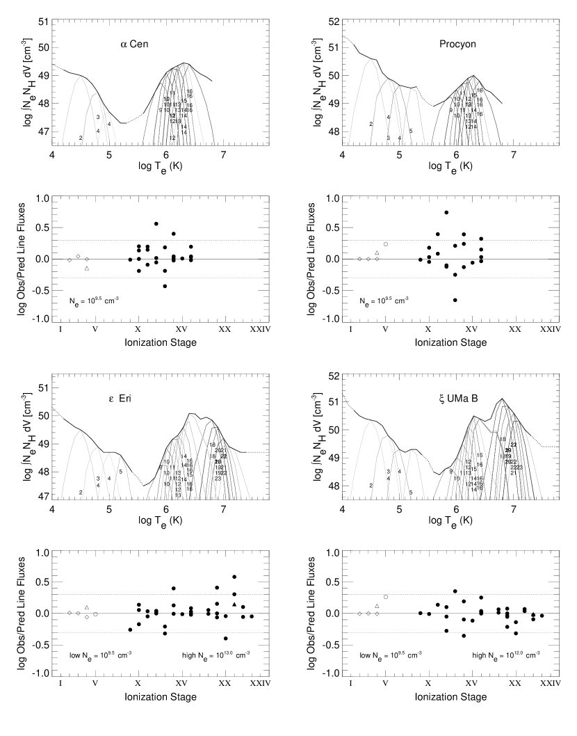
Figure 5: (a)Upper panels: EMD for the summed EUVE spectrum combined with the IUE spectrum for each star. Thin lines represent the relative contribution function for each ion (the emissivity function multiplied by the EMD at each point). Lower panels: Observed-to-predicted line ratios for the ion stages in top figure with S/N greater than 3. The dotted line denotes a factor of 2. Symbols used are open circles for N, diamonds for C, and open triangles for Si. Fe lines with S/N higher than 4 are denoted with filled circles, solid triangles for those with S/N between 3 and 4, and the plus sign (+) for S/N less than 3. Electron densities used in the calculation of the EMD are shown; if a value is not given, then the density was taken as 10¹² cm^-3.

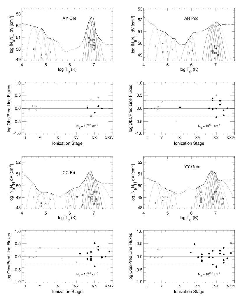
Figure 5: (b) continued.

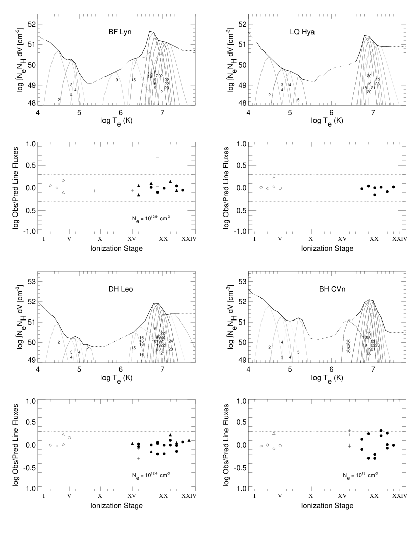
Figure 5: (c) continued.

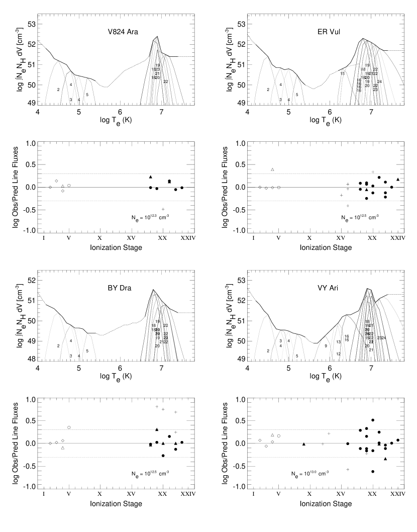
Figure 5: (d) continued.

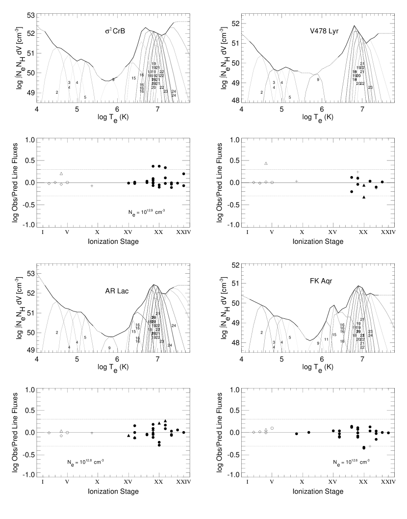
Figure 5: (e) continued.

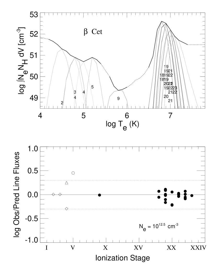
Figure 5: (f) continued.

We performed a line-based analysis of the emission spectra in order to calculate the EMD ($\int N_{e}N_{H}dV$ cm^-3, where $N_{e}$ and $N_{H}$ are electron and hydrogen densities, in cm^-3) corresponding to the observed fluxes. In contrast to ROSAT and ASCA measurements, which assume coronal models with only 2 or 3 temperatures, EUVE gives information on a continuous set of ionization states. In fact, all stages of iron ionization are represented from Fe IX through Fe XXIV except for Fe XVII, which has no strong transitions in the EUV spectral range. We used the line emissivities calculated from Brickhouse et al. (1995) for the EUVE iron lines, based on a solar iron abundance of 7.67 (Anders & Grevesse, 1989). Line emissivities from Raymond (1988) are used for the (non-iron) lines formed in the UV region. Theoretical fluxes were calculated using the assumed EMDs (see Dupree et al., 1993; Brickhouse & Dupree, 1998, and references therein) which were then iterated to obtain the EMD that best matches the observed fluxes. Generally agreement is better than a factor of two. It is important to note that we have integrated over the entire atomic emissivity function for each line in order to predict the model fluxes, and do not simply assume formation at a single temperature or temperature range. Iron lines severely contaminated by lines of other elements and some complex blends have been estimated by using the Astrophysical Plasma Emission Code (APEC) v1.10 (Smith et al., 2001). These are excluded from the EMD analysis as marked in Table 3. Figure 5 shows the EMD of summed spectra of the stars in the sample. Values used for the EMD are given in Tables 7 and 8, with a simple characterization suggested in Table 9.

4 Results

4.1 Low activity levels

In this group we include stars showing a spectrum dominated by lines formed at
log T(K)$\sim$5.8–6.5 (Fe IX–XVI), although with different contributions from the lines formed at higher temperatures (see Figs. 2a, 3). In the EMD derived for these stars, $\alpha$ Cen represents the lowest activity level observed in the sample, both in the transition region and in the corona. Procyon also has low levels in the corona, but the transition region EMD is comparable to that observed in more active stars (see § 5). Finally, $\epsilon$ Eri and $\xi$ UMa have high emission measure in the two temperature ranges, such that their EMDs represent an intermediate step towards the second group included in the sample.

4.1.1 $\epsilon$ Eri

$\epsilon$ Eri (HD 22049, HR 1084) is a relatively young star ($\sim$1 Gyr) showing high levels of activity. The effects of the dead spot prevent an analysis of the seasonal (i.e. year-to-year) variations of the light curves, but small scale variations can be seen with a frequency of $\sim$1–1.5 days, and some flaring activity could be present in the second part of the 1995 observations (Fig. 1).

Studies of the EUVE observations have been carried out by Laming, Drake, & Widing (1996) and Schmitt et al. (1996). Laming et al. (1996) derived the emission measure of each individual line as if it were emitting only at its maximum temperature thus obtaining an upper limit to the EMD value. This model peaks at log T(K)$\sim$6.5. Densities derived from Fe XIV line ratios (Laming et al., 1996) yield a value of log N_e(cm^-3)$\sim$9.5 at log T(K)$\sim$6.2, similar to results found by Schmitt et al. (1996).

We added all the available EUVE data of $\epsilon$ Eri in order to improve the statistics of the spectra, and the accuracy of the EMD. Although the EMD calculated (Fig. 5) indicates a peak around log T(K)$\sim$6.4, a range of values of the EMD predicts very similar line fluxes. It is difficult to distinguish a peak around log T(K)$\sim$6.5, from two peaks at log T(K)$\sim$6.4 and log T(K)$\sim$6.8. In order to identify a preferred EMD model, it would be optimum to use lines with a maximum of emission around log T(K)$\sim$6.5–6.7 such as Fe XVII which are not available in the EUVE spectral range.

The electron density calculated from the Fe XXI lines (3$\times$10¹³ cm^-3, see Table 6) points towards the presence of two kinds of structures at log T(K)$\sim$6.2 and log T(K)$\sim$7.0, because the inferred densities differ by $\sim$4 orders of magnitude, although some caution must be exercised in the interpretation of the measured electron density at high temperatures (see § 5) in this star (the adopted value in the EMD was log N_e[cm^-3]$\sim$13.0). The observed levels of EUV/flaring activity are higher than the flux levels of the quiet Sun, creating different conditions for the atmosphere of the planet found by Hatzes et al. (2000) associated with $\epsilon$ Eri.

4.1.2 Procyon

Procyon ($\alpha$ CMi, HD 61421, HR 2943) is an F5 IV-V star frequently used for comparison with the Sun. Its rotational period of 9.06 d is estimated from a v$\cdot$sin i=6.1 $km\ s^{-1}$ (de Medeiros & Mayor, 1999). The DS light curve of Procyon shows the presence of short-term modulation in a non-periodic time pattern of $\sim$14 hr in 1993 (Fig. 1). The observations taken in 1999 show higher dispersion in flux values than in 1993 and 1994; however, this effect can be due to the increase of activity in the Sun, as has been found in other observations taken in 1999 and 2000. In any case it does not seem possible to attribute these variations to intrinsic changes in the star.

During the EMD fitting process in Procyon, some of the lines have shown larger discrepancies between the observed fluxes and those predicted by the atomic model of Brickhouse et al. (1995). In particular, the Fe XII $\lambda$364.4 line seems too strong, as if blended, though the APEC model does not show an obvious candidate for blending.

4.1.3 $\xi$ UMa

$\xi$ UMa is a multiple system formed by four stars grouped in two spectroscopic binaries (Griffin, 1998) in a visual orbit of $\sim$60 yr. EUVE can not resolve the components. $\xi$ UMa A (HD 98231) is a spectroscopic binary with a P_orb=670.24 days (Griffin, 1998). A G0V star is the only star observed, and the companion is unknown – perhaps an M star (Griffin, 1998). $\xi$ UMa Aa shows low activity levels in the chromosphere, having very weak emission in the Ca II H & K lines (Montes et al., 1995). $\xi$ UMa B (HD 98230) shows an active spectrum, with stronger Ca II H & K emission lines coming from the observed G5V star, and a possible contribution from an unseen late-K dwarf (Griffin, 1998). The low value of the mass function (f[m]=0.000046M_⊙) found by Griffin (1998) points towards a very small value of the inclination ($\lesssim 11\arcdeg$), meaning a system observed almost at the pole. From the effective temperature (T_eff=5650 K, Cayrel de Strobel et al., 1994), and the typical values of stellar radii available in Gray (1992) relating radii and mass with spectral type, we estimate R= 0.95 R_⊙ for $\xi$ UMa B. IUE spectra from both components (Table 5) show that most lines are stronger in the B component of the system by a factor $\sim$2:1. Hence it is expected that the B component will be the main source of flux in the EUV wavelengths, but the A component is likely to have a non-negligible contribution of EUV light.

The light curve (Fig. 1) has been phased using the ephemeris given by Griffin (1998) for the A and B components, and adapted to follow the criteria of $\phi_{orb}$=0 corresponding to the primary star behind, resulting in T₀(HJD)=2,442,442.916, P_orb=3.980507 d. The DS light curves of $\xi$ UMa show some flaring activity, as well as semi-periodic fluctuations similar to those observed in other systems.

The Fe XVI line ratio in the MW spectrum (2.25$\pm$0.15) provides an accurate value of the hydrogen column density of $N_{H}=8.\pm 3\times 10^{17}$ cm^-2 (Fig. 4), lower than the value of $N_{H}=1.5\times 10^{18}$ cm^-2 estimated by Schrijver et al. (1995) from nearby stars. Fig. 5 shows the EMD calculated for this system. This is the most outstanding example of two peaks in the emission measure, with very similar values of the emission measure for each peak. This result fits the observed fluxes better than an EMD with only one peak at intermediate temperatures.

4.1.4 $\alpha$ Cen

As in the case of $\xi$ UMa, EUVE can not separate the light coming from $\alpha$ Cen A (HD 128620, G2V) and B (HD 128621, K1V). Hence, the observed light curve and spectra correspond to both stars. IUE spectra show higher flux levels in the A component (see Table 5) than in the B component, but EINSTEIN satellite x-ray observations show that the K1 star is the predominant source in the range 0.2–4 keV (Golub et al., 1982), with an approximate ratio 2:1.

The DS light curve of $\alpha$ Cen does not show any short-term change, and no flares are registered. Analysis of seasonal changes shows small variations, counting an increase in the flux by $\sim$15% from 1995 to 1997, while the 1993 observations are compromised by the dead spot. The hydrogen column density adopted is $N_{H}=6\times 10^{17}$ cm^-2, calculated by Linsky & Wood (1996) from Lyman $\alpha$ and Mg II h & k lines. As in the case of Procyon, disagreements occur between the observed and predicted fluxes in the Fe XII $\lambda$364.4.

The general shape of the EMD is similar to that of the Sun in the absence of flares, up to log T(K)$\sim$6.5 (see Reale, Peres, & Orlando, 2001). The electron density calculated from Fe X,  XII,  XIII, and  XIV lines in the range log T(K)$\sim$6.0–6.5 gives a value of log $N_{e}(cm^{-3})\sim$9.5 (Mewe et al. 1995; Drake, Laming, & Widing 1997).

4.2 Active stars

This group of stars includes those for which the EMD is clearly dominated by the emitting material at log T(K)$\sim$6.9 signaled by strong lines of Fe XVIII and Fe XIX, but with relatively small contribution from material at higher temperatures (compared to the most active stars in the third group). Capella (Dupree et al., 2002) is included in this group, and was also present in the sample of 28 stars studied in Sanz-Forcada (2001).

4.3 $\beta$ Cet

$\beta$ Cet (HD 4128, HR 188, K0 III) is a single star with an apparent low rotational velocity (v$\cdot$sin i= 3.5 $km\ s^{-1}$ Melo, Pasquini, & De Medeiros, 2001), but with surprisingly high levels of activity in X-rays. An estimate of the rotational period of 189.1 d can be deduced from the radius and inclination in Table The Structure of Stellar Coronae in Active Binary Systems and v$\cdot$sin i (Gray, 1989). Two sets of EUVE observations are available for $\beta$ Cet. An observation of 6 days during 1994 September shows a light curve with no significant variation, and a spectrum and EMD similar to that of active binary systems like Capella (Sanz-Forcada et al., 2002). A second set of observations taken during 2000 August shows flaring events in the DS light curve, and a level of emission much higher than in the 1994 campaign suggesting seasonal changes in the level of coronal activity of this star (Ayres, Osten, & Brown, 2001). The accumulated 808 ks of exposure time in the SW spectrum makes it the longest stellar observation with EUVE, and allows the analysis of a high-quality spectrum. Ayres et al. (2001) applied models based on upper-limit EMDs to the observed spectra of quiescence and flaring stages during this set of observations. These authors report a total exposure time of 645 ks, well below the exposure time calculated from archival data. This affects the fluxes reported by Ayres et al. (2001), which are larger than fluxes reported here by $\sim$15-35 %. No details are given by these authors on how well their model predicts the line fluxes, and during flaring stages their model spectrum seems not to accurately match some of the observed lines, including the density sensitive lines.

The EMD derived from the summed 2000 spectrum yields one of the best fits of the sample (see Fig. 5), although the lack of MW and LW spectra containing the Fe XV, Fe XVI and Fe XXIV lines, weakens the constraint on the EMD at log T(K)$\sim$6.5 and log T(K)$\sim$7.3. The resulting EMD shows clear differences with respect to the 1994 observations in the temperature range available in this observation, exhibiting a higher EMD mainly for temperatures higher than the bump at log T(K) $\sim$ 6.8 (see Sanz-Forcada et al., 2002).

4.3.1 AY Cet

AY Cet (HD 7672) is an RS CVn system with the EUVE flux dominated by a G5III active star, and a faint white dwarf companion with negligible flux contribution in this band. Schrijver et al. (1995) had difficulties applying a global fit to the noisy spectrum of AY Cet, and only the assumption of a low iron abundance allowed a result without a false “hot tail” in the EMD. The global fit yielded an EMD peaking at log T(K)$\sim$7.0. Our EMD modeling indicates a peak at log T(K)$\sim$6.9 (Fig. 5) with no “hot tail.” The shape of our EMD does not depend on abundances, since we use only Fe lines.

4.3.2 AR Psc

AR Psc (HD 8357, G7 V + K1 IV) has a shorter photometric period (P_phot=12.38 days; Cutispoto, Messina, & Rodonò, 2001) than the orbital period of 14.3023 days (Fekel, 1996), something unusual among RS CVn stars. Fekel (1996) proposed that AR Psc has not yet arrived on the main sequence to explain the lack of synchronization between the two periods. The EUVE observations of AR Psc with the DS (Fig. 1) reveal the persistence of an active region during a full rotational period. This active region is visible around JD$\sim$2,450,690.2 and JD$\sim$2,450,702.5, approximately the duration of the optical photometric period. Enhanced emission is also observed after the second appearance of this active region; this feature can not be unambiguously considered as a flare since the low enhancement of light ($\sim$50%) does not match the duration of the event ($\sim$1 day) when compared to other flares of similar duration (Osten & Brown, 1999; Sanz-Forcada et al., 2002).

There is much uncertainty in the hydrogen column density used for this star. A value of $N_{H}=2\times 10^{18}$ cm^-2 is assumed, estimated from column densities measured in nearby stars (Fruscione et al., 1994). AR Psc shows a fairly small bump in the EMD (Fig. 5), but peaking at a higher temperature than usual, at log T(K)$\sim$7.1. A better knowledge of the hydrogen column density is needed to specify the EMD particularly in the lower T regions defined by the iron lines at long wavelengths.

4.3.3 CC Eri

Similar to other systems observed in this sample, small-scale variability is present in the light curve of CC Eri (HD 16157, K7 V + M3 V), with non-periodic variations of 10–14 hr (Fig. 1). A short-duration flare could be present at JD$\sim$2,449,977.5. A value of $N_{H}=2.6\times 10^{18}$ cm^-2 was estimated by Pan & Jordan (1995) from the distance to the star and the average hydrogen column density. Amado et al. (2000), using this value, derived an upper limit to the EMD based on the temperature of maximum emissivity of IUE and EUVE spectral lines. Their derived EMD has a minimum around log T(K)$\sim$5.0 and a peak at log T(K)$\sim$6.8.

In the EMD we calculate with the whole emissivity function, the resulting distribution (see Fig. 5) shows a minimum at higher temperatures (between 5.5 – 5.8 dex), and an apparent overabundance of nitrogen is indicated by the N V $\lambda$1240 line, similar to the cases mentioned in Sanz-Forcada et al. (2002). The local enhancement in the EMD occurs at log T(K)= 6.8.

4.3.4 YY Gem

YY Gem (Castor C, HD 60179C) is a well known active system with two M dwarf stars in the double-lined spectrum. The DS light curves are characterized by the presence of many short flaring events (at least 7), including an enhancement by a factor of at least $\sim$9 at the very end of the observation (Fig. 1). Lower flux levels are displayed in the right panel to show the small-scale variability. This system has an orbital inclination of 86.3$\arcdeg$ (see Table The Structure of Stellar Coronae in Active Binary Systems), making it one of the best targets to search for rotational modulation and eclipses, as have been found with ROSAT (Schmitt, 1998). But the presence of frequent flaring, along with the noise found in the data, makes it difficult to find such evidence from the present observations.

The hydrogen column density towards nearby stars (Fruscione et al., 1994) suggests a column density of $N_{H}\sim 2.5\times 10^{18}$ cm^-2 to YY Gem, but this value seems to be high compared to nearby stars in our sample. The use of the Fe XVI line ratio ($\lambda$335/$\lambda$361) in the MW (1.8$\pm$0.3) yields an upper limit to the column density of $N_{H}\lesssim 6\times 10^{17}$ cm^-2 (Fig. 4). In view of these divergent results, we use the upper limit given by the Fe XVI line ratio, since it represents a direct measurement towards this star.

The EMD of the system (see Fig. 5) can be used to predict the Ar XV $\lambda$221.15 line using APEC and good agreement is found, assuming [Ar/Fe] 0.8 (a noble gas enhancement) and a solar oxygen abundance (Anders & Grevesse, 1989). Also, the complex blend at $\lambda$192 Å includes the Fe XII $\lambda$193.51 line, which may contribute $\sim$40% of the observed flux. These lines give some information regarding the stellar EMD near log T${}_{e}(K)\sim$6.3, although a better determination of the ISM absorption would be helpful.

4.3.5 BF Lyn

Variations by up to $\sim$20% with respect to the average value are observed in the light curve of BF Lyn (HD 80715, K2 V + dK), suggesting the presence of small-scale modulation in a semi-periodic pattern. As in the case of YY Gem, the value of the hydrogen column density towards BF Lyn is very uncertain, although the presence of the Fe XVI lines makes possible an estimate from their ratio (1.54$\pm$0.63) of $N_{H}\lesssim 5\times 10^{17}$ cm^-2, as shown in Fig. 4. Since the S/N of these lines is quite low, an intermediate value to that reported in nearby stars (similar to those in the case of YY Gem) has been adopted. The assumed value in the EMD calculations is $N_{H}=1.5\times 10^{18}$ cm^-2, more consistent with the EMD shape estimated when lines at long wavelengths are excluded from the fit.

4.3.6 LQ Hya

LQ Hya (HD 82558) is one of the single stars included in the sample. The youth of this star appears to be the main cause of the high levels of activity observed (see Montes et al., 1999, and references therein). The EUVE light curve (Fig. 1) shows variations by a factor of 2 during the “quiescent” state of the corona, and also two impulsive flares (intense flares of short duration) are present. The variations of the “quiescent” corona do not follow a clear periodic pattern, and are not related to the photometric period of 1.63 days (Cutispoto et al., 2001), but optical modulation is present on a scale of $\sim$1.2 days.

Wood et al. (2000) find an abnormally high value of the hydrogen column density of $N_{H}=1.1^{+0.5}_{-3.1}\times 10^{19}$ cm^-2, from an analysis of Lyman $\alpha$ and Mg II h & k lines. Since the Mg lines could be affected by stellar activity and and circumstellar gas, and data from nearby stars seems to disagree strongly with these values, we used the conservative value given by the lower limit, $N_{H}=8\times 10^{18}$ cm^-2. Given the lack of lines at longer wavelengths in the spectrum of LQ Hya (that could be affected even more by uncertainties in the adopted value of $N_{H}$), changes in the shape of the EMD due to such uncertainties will be minimal, leading mainly to a vertical displacement of the EMD. Good agreement is obtained between the predicted and observed fluxes (see Fig. 5).

4.3.7 DH Leo

The observed 1995 light curve of DH Leo (HD 86590) shows much variability (changes by up to $\sim$37% from the average value, Fig. 1), and some short flare-like events occur as well. Stern & Drake (1996) proposed that rotational modulation could be present in these observations. The Fe XVI line ratio does not provide an accurate value of the column density in DH Leo since the 361Å line has poor statistics. But the low flux observed in this line points to a rather high column density. Values of nearby stars in Fruscione et al. (1994) suggest $N_{H}\sim 1\times 10^{18}$ cm^-2. On the other hand, Diamond, Jewell, & Ponman (1995) deduced a wide range of values of $N_{H}=4.^{+28}_{-N/A}\times 10^{18}$ cm^-2 obtained from a fitting to ROSAT spectra. An intermediate value with those of nearby stars has been adopted, $N_{H}\sim 2\times 10^{18}$ cm^-2.

4.3.8 BH CVn

BH CVn (HD 118216, HR 5110) shows a remarkable pattern of variability in the EUVE light curve (Fig. 1), with semi-periodic variations of $\sim$20–30 hr.

There is much uncertainty in the determination of the hydrogen column density in the direction of BH CVn. Spectral fits to ROSAT data yield very high column densities (over $N_{H}\gtrsim 1\times 10^{19}$ cm^-2, Diamond et al. 1995; Graffagnino, Wonnacott, & Schaeidt 1995), although this is not a reliable method to determine $N_{H}$. The Fe XVI line ratio of 1.45$\pm$1.17 does not point to an accurate value either, due to the low S/N of the lines, but the upper limit of this ratio corresponds to $N_{H}\sim 3\times 10^{18}$ cm^-2 (Fig. 4). On the other hand, the values derived from nearby stars (Fruscione et al., 1994) yield a lower estimate of $N_{H}\sim 7\times 10^{17}$ cm^-2. As a compromise among these values we have chosen the upper limit given by the Fe XVI line ratio, $N_{H}=3\times 10^{18}$ cm^-2, also consistent with Mitrou et al. (1997). The calculated EMD (Fig. 5) shows a bump similar to other stars, with a decreasing EMD at higher temperatures.

4.3.9 V824 Ara

About 2.5 days of DS light curve observations were obtained for V824 Ara (HD 155555) in 1996. The low flux (note the 3000 s binning) gives quite large error bars (see Fig. 1). Nevertheless, it is possible to identify some modulation coincident with the orbital and photometric periods of the system ($\sim$1.68 days). Local maxima appear at phases 1.0, 1.5, and 2.0, consistent with orbital modulation, although flare-like variability can not be excluded.

The small number of lines present in the spectrum of this young active binary system makes the estimate of the EMD less accurate. Airapetian & Dempsey (1998) made an analysis based on the peak of the emissivity function in order to calculate minimum values of the emission measure. The resulting EMD (Fig. 5) shows a poorly constrained bump near log T(K)$\sim$6.9. The electron density (Table 6) derived from the ratio Fe XXI $\lambda$102.22/$\lambda$128.73 is not very reliable, since the $\lambda$102.22 line flux was measured including a blend with the Fe XIX $\lambda$101.55 line. The flux of the Fe XIX line was estimated from the EMD to account for its contribution to the blend.

4.3.10 ER Vul

The DS light curve of the partially eclipsing system ER Vul (HD 200391) shows some variability, as well as flare-like activity at a low level. Osten & Brown (1999) suggested the variations resulted from small-scale flares, and found no eclipses or periodicities in this BY Dra-type system. The EUVE observations span $\sim$10 epochs of the binary enhancing detection of periodicity. A power spectrum of the DS light curve (with flaring portions omitted) shows a maximum corresponding to the optical period. When the DS light curve is phased to this period, there is modulation at most by a factor of 5 with a suggestion of absorption near phase 0.5 when the G0V component is partially occulted by the G5V star. Thus the corona may be more compact in the hotter star of ER Vul.

There is much uncertainty in the value of the hydrogen column density towards ER Vul, since the values towards nearby stars reported in Fruscione et al. (1994) show discrepancies. The value adopted by Rucinski (1998) of $N_{H}=3\times 10^{18}$ cm^-2 has also been used in this work. This uncertainty could affect the determination of the slope at temperatures below the bump in the EMD because that region is defined by lines at longer wavelengths where the impact of interstellar absorption is largest.

4.3.11 BY Dra

The DS light curve of BY Dra (HD 234677) covered an orbital period of this system (Fig. 1). Although some variation occurs that could correspond to the rotational period of the system of $\sim$3.83 days (see Table The Structure of Stellar Coronae in Active Binary Systems), several flares prevent a clear identification of rotational modulation.

Values from nearby stars suggest a quite high hydrogen column density ($N_{H}=5\times 10^{18}$ cm^-2), consistent with the lack of flux detected in the MW spectrum, probably due to ISM absorption. We have used this value in the absence of other evidence. Unless large differences in the hydrogen column are present with respect to this assumed value, there will be only a minimal influence on the shape of the EMD (Fig. 5).

The electron density calculated for BY Dra makes use of lines with S/N lower than 3, and hence these values are not very reliable. The EMD is fit to emissivities at log N_e(cm^-3)$\sim$12, which gives a good fit to the density-sensitive resonance line Fe XXI $\lambda$128.7.

4.4 Very active stars

Some stars in the sample contain substantial amounts of material at temperatures beyond log T(K)$\sim$7.0, sometimes with emission measures even larger than the values at log T(K)$\sim$6.9. Most of those stars included in Sanz-Forcada et al. (2002), UX Ari, V711 Tau, $\sigma$ Gem, II Peg, and AB Dor belong in this category of high activity. The presence of material at these temperatures is determined by the Fe XXIII and Fe XXIV lines. Fe XXIV occurs in the MW spectrum which frequently suffers from insufficient exposure time in current data sets. Future observations, for instance with Chandra or XMM-Newton, could reveal high temperature emission that was not detected in short exposures with EUVE.

4.4.1 VY Ari

The DS measurements of VY Ari (HD 17433) are compromised by the dead spot of the DS detector during the observation (Fig. 1). However, the SW light curve supports the modulation observed in the DS light curve, with a decrease of flux of $\sim$60% during the observation.

We have used the same value for the hydrogen column density as in the case of the nearby star UX Ari ($N_{H}=1.5\times 10^{18}$ cm^-2, Sanz-Forcada et al., 2002). In constructing the EMD, we find that the predicted fluxes in two of the Fe XX lines do not well match the measured values. While the observed flux of $\lambda$110.63 is too strong, the $\lambda$121.83 transition is too weak. These lines could be affected by other blends not included in the analysis. In any case, this makes the electron density (cm^-3) of 13.8 dex deduced from the ratio Fe XX $\lambda$110.63/($\lambda$118.66+$\lambda$121.83) less certain, and points towards a lower value, probably closer to that deduced from Fe XXI ratios of $\sim$12.5 dex (see Table 6). The resulting EMD (Fig. 5) is not very sensitive to the use of a different electron density in this range (the adopted value was log N_e[cm^-3]$\sim$13.0).

4.4.2 $\sigma^{2}$ CrB

The DS light curve of $\sigma^{2}$ CrB (HD 146361) shows intense flares (Fig. 1), and also small-scale variability on the order of several hours ($\sim$6–10 hr). The flare timing of this observation was analyzed in detail by Osten & Brown (1999) and Osten et al. (2000).

The good S/N achieved in the Fe XVI lines in the MW spectrum allows an accurate determination of the hydrogen column density, resulting in a value of $N_{H}=2.5^{+1.5}_{-0.9}\times 10^{18}$ cm^-2 (Fig. 4), consistent also with Mitrou et al. (1997). Fig. 5 shows an EMD that reflects a very hot corona, with an increasing value at temperatures higher than the “bump.” Also the general level of the EMD is comparable to that of RS CVn systems composed of subgiants, whereas the components of $\sigma^{2}$ CrB are dwarf stars, demonstrating their unusually high activity levels.

4.4.3 V478 Lyr

The lack of good statistics in the DS light curve (Fig. 1) of V478 Lyr (HD 178450) masks possible low level variability. Variations of $\sim$25% with respect to the average flux are found in the data, with no clear evidence of DS eclipses. The system has an inclination of 83$\arcdeg$ and undergoes partial eclipses (Strassmeier et al., 1993).

An intermediate value of the hydrogen column density, $N_{H}=4\times 10^{18}$ cm^-2 has been used from estimates for stars nearby in the sky (Fruscione et al., 1994). The EMD is not affected significantly by the uncertainties in $N_{H}$ (see Table The Structure of Stellar Coronae in Active Binary Systems), since all the emission line fluxes are taken from the SW spectrum, where interstellar optical depths are small. Although the number of lines measurable with reliable statistics in this system is small, it was possible to construct an EMD similar to other stars in the very active group.

4.4.4 AR Lac

AR Lac (HD 210334) is an eclipsing binary with two active stars (G2IV/K0IV) that shows chromospheric emission originating from the K0IV star (Montes et al., 1997). The measurement of the primary eclipse depth in the 1993 and 1997 observations (Fig. 1) reveals a contribution by the K0IV star of at least a $\sim$37% (measured at the center of the primary eclipse) of the total EUV light. The partial contamination of the light curve by the dead spot in 1993, and the presence of flares around phases x.5 in 1993 and 1997 prevent a reliable measurement of the secondary eclipse. The light curve in the 2000 observations, reported by Pease et al. (2001), is dominated by a large flare. The EUV flux increases by at least a factor of $\sim$17 from the quiescent level. A total net energy release of 2.0$\times 10^{35}$erg is found in the range 80–170 Å, after the subtraction of the “quiescent” contribution of the 1993 and 1997 summed observations, following the method explained in Sanz-Forcada et al. (2002). The flux obtained before the subtraction of the quiescent contribution was 4.4$\times 10^{35}$erg. A complementary analysis of the observations in 2000, with partially simultaneous Chandra data can be found in Huenemoerder et al. (2002).

During the 2000 flare, AR Lac shows an increase in flux in the hottest lines of the EUVE spectrum, and some increase also in the continuum level. There may be an increase of the average density measured during the flaring observation as indicated by Fe XXII but not confirmed by other ratios (see Table 6).

Although there is some uncertainty in the measurement of the Fe XVI lines (especially the $\lambda$360.8 line), we use the hydrogen column density derived from their flux ratio (2.5$\pm$0.8) found in the MW spectrum corresponding to the 1993 and 1997 observations co-added (Fig. 4). The resulting value $N_{H}(cm^{-2})=1.8\times 10^{18}$ is consistent with the column density of $N_{H}(cm^{-2})=2\times 10^{18}$ assumed by Griffiths & Jordan (1998), calculated from nearby stars.

Kaastra et al. (1996) and Griffiths & Jordan (1998) used the 1993 data to obtain EMDs with a clear peak around log T${}_{e}(K)\sim$6.9, although they differ in the distribution at other temperatures. A preliminary analysis of the 1997 data alone was made by Brickhouse et al. (1999). The addition of the 1993 and 1997 data allows the analysis to be extended to almost the whole range of log T${}_{e}(K)\sim$4.0–7.4. The 2000 data are used to compare a flaring sequence to the “quiescent” observations of 1993 and 1997.

Fig. 5 displays the EMD calculated from the 1993 and 1997 summed data. The height of the bump is less prominent during the flare because the material at higher and lower temperatures increases. However the value of the EMD at the bump remains constant demonstrating its stability in the corona (Fig. 6). This reinforces the hypothesis of large flares as phenomena unrelated to the bump at log T${}_{e}(K)\sim$6.9, suggested previously by Sanz-Forcada et al. (2002).

4.4.5 FK Aqr

The nearby active binary system FK Aqr (HD 214479) is composed of two M dwarf stars orbiting with a $\sim$4 day period. The DS light curves in the 1997 campaign show frequent flaring activity (Fig. 1), with impulsive flares of short-duration ($\sim$15 hr) that are quite strong (increases by up to a factor of 5). The presence of these flares blurs any possible modulation related to rotation. In contrast, the 1994 observations show a quiet corona, and only a small flare is present. Some enhancement of flux arises during the second half of the orbital period in 1994, probably due to the presence of an active region in the line of sight, as Stern & Drake (1996) proposed. Values of inclination and photospheric radii of this system can be inferred in a first approximation by assuming that the pair of M2V/M3V dwarfs follows the relations derived by Gray (1992). This would imply stellar radii of 0.55/0.52 R_⊙, and with the typical mass of 0.42 and $m\,sin^{3}i=0.27$ for the primary, an inclination of i$\sim$60$\arcdeg$ can be estimated.

There are no direct measurements of the interstellar column density towards this system, but stars nearby in the sky (Fruscione et al., 1994) suggest a value of $N_{H}=7-10\times 10^{17}$ cm^-2. The Fe XVI line ratio in the MW spectrum (1.96$\pm$0.20) provides an upper limit to the hydrogen column density of $N_{H}=7\times 10^{17}$ cm^-2 (Fig. 4). This value was assumed here. Fig. 5 shows a remarkably well-fitted EMD, with a first bump in temperature similar to the solar EMD (see Reale, Peres, & Orlando, 2001), and the typical second bump found in most of the stars in this sample around log T${}_{e}(K)\sim$6.9.

5 Discussion

One goal of this research is to identify the stellar parameters that influence the coronal structures. Systematics of the light curves, EMD, and densities are discussed below. We then compare the underlying patterns of coronal structure to the properties of the stars.

5.1 Light Curves

The intrinsic variability found in the light curves of these systems makes it difficult to confirm seasonal (year-to-year) changes in the EUV emission. Among the quiet stars, only $\alpha$ Cen shows some small decrease in the light curve flux (by $\sim$15%) between 1995 and 1997, but the observations are too short to attribute these changes to seasonal variations. The fluctuations found in the quiescent emission of II Peg are of order $\sim$50% (Sanz-Forcada et al., 2002), although in this case the effects of intrinsic variations could be more important. The clearest case for seasonal fluctuations is found in the single giant star $\beta$ Cet, which in 1994 is very quiet for the 6.4 day observation. The DS flux is about a factor of 2 lower than in 2000 (Sanz-Forcada et al., 2002), and Ayres et al. (2001) identify at least 5 flaring events during the $\sim$34 days of monitoring in 2000 (see Fig. 1). Some line fluxes are enhanced by more than 50% (a factor of 5 for Fe XXIII/XX $\lambda$132.85!). The intrinsic variability found in stars like $\sigma$ Gem, LQ Hya or FK Aqr, even in the absence of large flares, makes it difficult to confirm seasonal changes.

Signatures of rotation are clearly found in the eclipses of AR Lac, and might be present in the light curves of AR Psc, ER Vul, VY Ari and BY Dra. Marginal evidence for modulation was found previously in II Peg, UX Ari, $\sigma$ Gem, and AB Dor (Sanz-Forcada et al., 2002). Additional short-term variations are found in many stars in this sample, indicating non-periodic changes on time scales between 0.3 and 1.5 days. Instrumental effects can be rejected in the case of V711 Tau, and these variations are likely to be real for many stars in the sample, including V711 Tau, LQ Hya, $\sigma^{2}$ CrB and BF Lyn (see Fig. 1). This variability can be attributed to flare-like phenomena on a small scale, perhaps reflecting the existence of many solar-like flares (shorter duration and intensity than the large flares which are well observed in these stars).

5.2 Emission Measure Distribution

A continuous distribution of material occurs in these coronas, spanning 3 decades of temperature or more. It is now clear that the earlier simplifications of 1-T or 2-T coronal models resulted from insufficient spectral resolution and/or incomplete global models preventing identification and analysis of the wide range of excitation and ion stages naturally present in the coronae of cool stars. Results assembled in Fig. 4 show the distribution of material to be generally similar among active cool stars, whether single or binary. A decrease in the EMD between 10⁴K and 10^∼5.5K and then an increase, with one or more local enhancements between 10⁶ and 10⁷K represent the structure of the stellar chromosphere, transition region, and corona.

However, a detailed comparison shows that clear differences appear at temperatures above log T(K)$\sim$5.2. Only $\alpha$ Cen, with a solar-like EMD, has a distribution that begins increasing above temperatures as low as log T(K)$\sim$5.2. The remaining stars in the sample have the minima in the EMD at higher temperatures [log T(K)$\sim$5.8]. This difference between the minima of the Sun and Capella was noted from the first EMD derived from EUVE (Dupree et al., 1993). We note that the Sun shows minima at different temperatures for different types of structures. For example, solar coronal holes frequently have a higher temperature EMD minimum than do active regions.

At temperatures above 10⁶ K, additional structures are found, characterized by local enhancements of the EMD over narrow temperature ranges. Such a feature was also discovered in Capella and labeled the “bump” (Dupree et al., 1993; Brickhouseet al., 2000), and have been identified with high latitude coronal features (Brickhouse & Dupree, 1998). Several stars show a local enhancement at log T(K)=6.2 reminiscent of the temperature of the solar corona in addition to a bump at log T(K) =6.8. The presence of this second high temperature bump is unambiguously found in 25 out of 28 stars in the sample (all except $\epsilon$ Eri, $\alpha$ Cen, and Procyon). Clearly, these represent a fundamental coronal structural feature. Finally, the stars with an increasing EMD beyond log T(K)$\sim$6.9 represent the very active classification. The progressive addition of hotter material marks the increase in activity level.

Given the different physical sizes of the stars in the sample, it is useful to evaluate the emission measure weighted by the emitting surface of the stars (4$\pi$[R${}_{1}^{2}$+R${}_{2}^{2}$]), so that the emission measure per unit area defines an effective column density of coronal material. Fig. 7 shows 6 cases representative of different degrees of activity, weighted by the size of the emitting stars – the “column” EMD. Procyon shows the same amounts of material as $\alpha$ Cen at temperatures above log T(K)$\sim$6. Except for $\alpha$ Cen, the chromospheric structures are similar, while the greatest divergence occurs at the highest temperatures.

5.3 Electron Density

Electron densities derived from line ratios at log T(K)$\sim$7.0 indicate values of
log $N_{e}(cm^{-3})\gtrsim$12. There is considerable dispersion in the data for values of log $N_{e}(cm^{-3})\gtrsim$13, as noted previously for Capella (Brickhouse, 1996), as well as for densities at lower temperatures in solar active regions (Brickhouse et al., 1995). Numerous observational issues compromise these results. The presence of blends not well evaluated in the models and uncertainties in the placement of the continuum used as a base for the line flux measurements clearly influence some of these measurements. In particular, the Fe XX line ratios show a systematically higher density than other iron line ratios at similar temperatures, as well as a poorer fit of the emission measure; therefore more caution must be taken with the results from this ion. While the atomic models for the diagnostic line ratios have been benchmarked under controlled conditions (Fournier et al., 2001), higher resolution spectra with good signal to noise, are needed.

Nevertheless, density diagnostics from several stars in this sample have good statistics and consistency among several diagnostics, e.g. VY Ari and CC Eri discussed here and V711 Tau and $\sigma$ Gem (Sanz-Forcada et al., 2002). Given these results, a “conservative” value of log $N_{e}(cm^{-3})\sim$12 seems plausible. We note that lower values of density at log T(K)$\sim$6.2 found by several authors in different stars (see § 4.1 and, e.g. Canizares et al., 2000) are not necessarily inconsistent. Brickhouse (1996) used similar results for Capella from Fe M-shell and L-shell diagnostics, and suggested the presence of two different types of structures.

The densities calculated at log T(K)$\sim$7.0, in combination with the emission measure values at that temperature, can be used as a first approximation to estimate the scale size of the emitting structures (Sanz-Forcada et al., 2001), with the caveat that there is no information on their geometry and filling factors. The calculations show in all cases that such structures are small ($\lesssim$0.02 R_∗), both for dwarfs and giant stars. Small structures have been found also by several authors, e.g., Dupree et al. (1993), Bowyer, Drake, & Vennes (2000), Phillips et al. (2001) and references therein.

Current loop models cannot accommodate the presence of the high electron densities found here at coronal temperatures. Observations of the Sun only detect such high values during solar flares (Phillips et al., 1996). Light curves from EUVE do not have enough signal in short integration periods to detect the presence of fast solar-like flares in stars, so it is not possible to differentiate such flares from the emission in quiescence. The presence of frequent solar-like flares in these stars can not be ruled out or confirmed with the present data. Such flaring could account for both the shape of the EMD and the high electron densities. A model of (continuous) nano-flare heating in the Sun can predict the shape of the EMD with a bump at log T(K)=6.8 (Klimchuk & Cargill, 2001), but with densities two orders of magnitude lower than observed here.

5.4 Comparison with Stellar Properties

For a quantitative comparison of these EMDs, we extract parameters of the distribution for comparison to physical properties of the systems. To define the temperature of the peak of the EMD, we consider the three largest values of the emission measure in the range log T(K)=5.8–7.3. The temperature defined for the peak and its emission measure were compared to the orbital periods of 30 stars, as shown in Fig. 8. This sample includes also the data from Capella (Dupree et al., 1993), 44 Boo (Brickhouse & Dupree, 1998), $\lambda$ And (Sanz-Forcada et al., 2001), the 6 stars (V711 Tau, II Peg, $\sigma$ Gem, UX Ari, AB Dor, and $\beta$ Cet) in Sanz-Forcada et al. (2002), and the Sun during solar maximum (Orlando, Peres, & Reale, 2000).

The temperature of the peak of the EMD (Fig. 8a) remains relatively constant at log T(K)= 6.9 for the binary stars and 3 single stars (AB Dor, LQ Hya, and $\beta$ Ceti). AB Dor and LQ Hya are young rapidly rotating effectively single stars. Beta Ceti appears as an anomaly with strong emission - an apparently single slowly rotating star - consistent with its classification as K0 III giant. It may be a clump star that experiences a regeneration of its magnetic dynamo, or it may be oriented pole-on to our line of sight, and the rapid rotation is not observable.

The mean electron densities at log T(K)=6.9 for the sample are shown in Fig. 8b. Density values range between 10¹²–10^13.5 cm^-3 with no systematic dependences on binarity or orbital period for the systems with P${}_{orb}<$20 d. There is no evidence for the highest densities in longer period systems, but only 3 objects are in that group.

Values of the EMD at the peak temperatures are shown in Fig. 8c and 8d. For binaries, the value of the EMD increases with increasing orbital period, as dwarf stars tend to have shorter periods in our binary sample, whereas the larger RS CVn subgiants and giants have longer periods. Scaling the emission measure at its peak value by the areas of the stars reveals the decrease in “column” EMD with increasing orbital period. There may be a saturation of the “column” EMD at periods less than 2.3 days where a constant value appears consistent with the data.

Line fits to the data are superimposed, indicating the best fit for all the objects,

$$log(EM_{peak}/area)=50.4-0.85\ logP_{orb}$$

and only those with period longer than 2 days,

$$log(EM_{peak}/area)=50.5-0.89\ logP_{orb}$$

where P_orb is given in days, EM in units of cm^-3, and area is defined by 4$\pi$[R${}_{1}^{2}$+R${}_{2}^{2}$] , with radius in solar units. In all cases a solar photospheric abundance was assumed. Since the absolute value of the emission measure peak depends on the iron to hydrogen abundance, this assumption requires testing. Furthermore, if there are substantial iron enhancements or depletions as a function of coronal temperature, the EMDs will need to be reconstructed accordingly.

We also plot in Fig. 9 the orbital periods of the systems against the EUV (80–170 Å) luminosity weighted by the bolometric luminosity (L_EUV/L_bol). The EUV luminosity was calculated from the integrated SW spectrum of the stars, corrected for the instrumental effective area and interstellar absorption. The bolometric luminosity results from the application of the bolometric corrections available in Flower (1996). This plot may be affected by uncertainties in the calculation of the bolometric luminosity. The EUV flux may arise from one star in a binary, yet the magnitude ($V$) and color ($B-V$) of the system are used to calculate the bolometric luminosity. The results in Fig. 9 show much dispersion. However, the general behavior of increasing $L_{euv}/L_{bol}$ with shorter period and a possible saturation at periods $\sim$ 1 day or less are consistent with studies of L_X/L_bol of active cool stars (cf. Walter & Bowyer 1981; Pallavicini et al. 1981; Fleming, Gioia, & Maccacaro 1989). An increase of flux in X-rays is generally found for faster rotators, with the relation becoming “flat” at some point at rotational periods between 1 and 10 days, marking a so-called “saturation limit”. In the sample considered here, a simple linear relation can fit the data, although the stars with fastest rotation ($\lesssim$ 2.3 d) follow a flatter distribution with period.

Our results suggest the presence of three kinds of structures, at temperatures of
log T(K)$\sim$6.3, $\sim$6.8, and log T(K)$\gtrsim$7.2, that dominate the emitting coronae of cool stars. Loop models predict a shape roughly similar to that deduced here from the combined UV and EUV analysis (cf. Sanz-Forcada et al., 2002). These models generally balance radiative losses by a heating function, and conduction redistributes energy along the loop. An emission measure would increase until the peak temperature of the loop, beyond which the amount of material would drop drastically. The addition of loops at higher temperatures can compensate for this drastic fall in the loop emission measure in order to reproduce the observed stellar EMD.

The classic view of static loops with fixed cross-section gives an EMD that increases linearly in the high temperature region, with a predicted slope of 1.5. But more complex loops, with expanding cross-section (Schrijver, Lemen, & Mewe 1989; Griffiths, N. W. 1999; Hussain et al. 2002) can account for larger slopes near the peak temperature of the loop, although not with high electron densities. Low activity stars, like the Sun, Procyon, or $\alpha$ Cen, would be dominated by solar-like loops, peaking at log T(K)$\sim$6.3, and with electron densities in the range log $N_{e}(cm^{-3})\sim$9–10.5 (Drake, Laming, & Widing 1995; Mewe et al. 1995; Drake et al. 1997). Solar-like flares can produce a bump in the EMD at temperatures around log T(K)$\sim$7.1 (Orlando et al., 2000; Reale, Peres, & Orlando, 2001). Stars such as Capella (Dupree et al., 1993) and FK Aqr are dominated by structures with maximum temperature around log T(K)$\sim$6.9 and log $N_{e}(cm^{-3})\gtrsim$12. Finally, only the most active stars show the possible presence (not well constrained with EUVE data) of hotter loops that could explain the observed emission of the hottest lines. These hot loops may be directly related to the existence of large flares in stars like UX Ari, $\sigma$ Gem, V711 Tau and II Peg (Sanz-Forcada et al., 2002). For the case of AR Lac presented here, the value of the emission measure increases during the flares at all temperatures, with only a slight increase in the EMD slope at the hottest temperatures (see Table 9).

It is significant that the high temperature enhancement (the “bump”) appears ubiquitous in the coronae of cool stars. Moreover the temperature of this enhancement is almost the same in a wide variety of cool stars. It is not clear why this happens. Gehrels and Williams (1993) noted a very small ($<$3%) inflection in a theoretical radiative cooling curve near 6$\times$10⁶K and suggested it might account for stable coronal structures. However these considerations apply when radiation dominates over conductive losses and when the abundances are photospheric. Both constraints may not apply in stellar coronae. Additionally, changes in the ionization equilibrium and atomic physics will impact such small details of the cooling curves. It is fair to conclude that current theoretical models can not reproduce the observed emission measure distributions with high densities.

6 Conclusions

1. Emission measure distributions (EMD) were derived from EUVE spectra of 22 active binary systems and 6 single stars. The overwhelming majority (25) of the stars in the sample show an outstanding “bump” – a local enhancement of the EMD – over a restricted temperature range. This bump occurs near log T_e (K)$\sim$6.8–7.0. Its presence does not depend on the luminosity class of the star or the activity levels present, and confirms a fundamentally new coronal structure.

2. The emission measure per unit area (“column” EMD) increases towards shorter orbital periods, with a possible “saturation” effect at periods less than  2.3 days.

3. Fe XIX–XXII line flux ratios, formed at log T${}_{e}(K)\sim$7 and measured in the summed spectra for each star indicate high electron densities (log $N_{e}[cm^{-3}]\gtrsim$12). In conjunction with lower densities found previously at lower temperatures, these results provide additional evidence for different structures in stellar coronae.

4. A second local enhancement of the EMD peaking at log T${}_{e}(K)\sim$6.3 could reflect the presence of solar-like loops in the corona of some stars in the sample, and dominates the EMD in $\alpha$ Cen AB, $\epsilon$ Eri, and Procyon.

5. Fe XXII–XXIV line fluxes indicate the presence of much hotter material at temperatures log T${}_{e}(K)\gtrsim$7 in some stars (VY Ari, $\sigma^{2}$ CrB, V478 Lyr, and AR Lac).

6. The derived EMDs suggest these stellar coronae are composed of solar-like magnetic loops (peaking at log T${}_{e}[K]\sim$6.3). The loops at log T${}_{e}(K)\sim$6.9 are not yet understood from loop models. Loops peaking at log T${}_{e}(K)\gtrsim$7.2 may be related to large flares.

7. Fluctuations in the EUV light curve of many stars in the sample are observed in a non-periodic 8–36 hr pattern, indicating the existence of frequent low-level variability.

Figure 1: DS light curves as a function of Julian Date (lower axis) and orbital phase (upper axis). We use the convention that at orbital phase 1.0 the primary star is located behind the secondary star (see Table The Structure of Stellar Coronae in Active Binary Systems); photometric phase is used in the upper axis for $\epsilon$ Eri and LQ Hya, and no periods are available for $\alpha$ Cen, Procyon, and $\beta$ Cet. Open circles mark data affected by the dead spot (and corrected by the DS to SW flux ratio, see § 2), while solid circles represent unaffected data. An average one-sigma error bar is shown as reference on the left side of each plot. Only points with S/N higher than 5 are plotted. The bin size is 600 s.

Figure 1: (b) continued.

Figure 1: (c) continued.

Figure 1: (d) continued.

Figure 2: (a) EUVE SW and MW spectra of the stars in the sample. Ion stages of iron are marked in the top panel. Spectra are smoothed by 5 pixels. Dotted lines indicate the zero flux level of each spectrum.

Figure 2: (b) continued.

Figure 2: (c) continued.

Figure 2: (d) continued.

Figure 3: AR Lac, $\beta$ Cet and LW spectra of 5 of the stars. Note that 2^nd order of the He I line is detected in the LW spectra at 608 Å.

Figure 4: Fe XVI $\lambda$335 and $\lambda$361 line flux ratios (in photon units) expected for different values of interstellar hydrogen column density (N_H), and observed ratios for several stars in the sample, with 1-$\sigma$ observational error bars.

Figure 6: Comparison between the EMD calculated from the observations on AR Lac in 1993+1997 and those in 2000.

Figure 7: EMD of selected stars normalized to the solar photospheric radius [EMD/$4\pi(R_{1}^{2}+R_{2}^{2})$= “column” EMD, assuming that both stars in binary systems contribute to the observed emission, with radii measured in R_⊙]

Figure 8: Orbital (or photometric) period relations with several features for 30 single and binary stars: (a) Temperature at the peak [3 largest values of the emission measure (EM)], (b) density at log T(K)$\sim$6.9, (c) EM at the peak, (d) EM at the peak per unit area [EM/$4*\pi*(R_{1}^{2}+R_{2}^{2})$], with radii in solar units. A solid line with the best fit to all the data has been plotted in (d), along with a dashed line representing the fit including only objects with period over 1 day. Filled circles represent binary systems, diamonds are single stars, and an open circle represents the Sun during the solar maximum (from Orlando et al., 2000).

Figure 9: Orbital period versus EUV (80–170 Å) luminosity weighted by the bolometric luminosity (see text). A solid line with the best fit to all the data has been plotted in (d), along with a dashed line representing the fit including only objects with period longer than 2 days. Filled circles represent binary systems and diamonds are single stars.

Table 1: Stellar parameters

Name	HD	Spectral Type	Porb(d)	Pphot(d)	i ($\arcdeg$)	NH(cm-2)	d (pc)	R⋆(R⊙)
$\beta$ Cet	4128	K0III	$\cdots$	$\cdots$	60:	2.2$\times 10^{18}$	29.4	15.1:
AY Cet	7672	WD/G5III	56.824	77.22	29	6.$\times 10^{18}$	78.5	0.12/9
AR Psc	8357	G7V/K1IV	14.3023	12.38	30:	2.$\times 10^{18}$	45.2	?/3.2
CC Eri	16157	K7V/M3V	1.56145	1.56145	42	2.6$\times 10^{18}$	11.5	0.65/0.41
VY Ari	17433	K3-4V-IV+?	13.198	16.23	60:	1.5$\times 10^{18}$	44.0	$\gtrsim$3.3/?
$\epsilon$ Eri	22049	K2V	$\cdots$	11.3	30:	1.3$\times 10^{18}$	3.22	0.75:
YY Gem	60179	dM1e/dM1e	0.814282	0.8143	86.3	6.$\times 10^{17}$	15.8	0.62/0.62
Procyon	61421	F5IV-V	$\cdots$	$\cdots$	32	1.6$\times 10^{18}$	3.50	2.06
BF Lyn	80715	K2V/[dK]	3.80406	$\sim P_{orb}$	66	1.5$\times 10^{18}$	24.3	$>$0.78/$>$0.78
LQ Hya	82558	K2V	$\cdots$	1.63	55	8.$\times 10^{18}$	18.3	0.8
DH Leo	86590	{K0V/K7V}K5V	1.070354	1.0665	78:	2.0$\times 10^{18}$	32.4	0.97:/0.67:
$\xi$ UMa B	98230	G5V/[KV]	3.980507	$\cdots$	11	8.0$\times 10^{17}$	8.35	0.95/?
BH CVn	118216	F2IV/K2IV	2.613214	$\cdots$	9	3$\times 10^{18}$	44.5	3.10/2.85
$\alpha$ Cen A	128620	G2V	79.90 yr	22	79.29	6.0$\times 10^{17}$	1.35	1.2
$\alpha$ Cen B	128621	K1V	79.90 yr	41	79.29	6.0$\times 10^{17}$	1.35	0.91
$\sigma^{2}$ CrB	146361	F6V/G0V	1.139791	1.1687	28	2.5$\times 10^{18}$	21.7	1.22/1.21
V824 Ara	155555	G5IV/K0V-IV	1.681652	1.682	55	6$\times 10^{18}$	31.4	1.38/1.29
V478 Lyr	178450	G8V/[dK-dM]	2.130514	$\sim P_{orb}$	82.8	4$\times 10^{18}$	28.0	1.0/?
ER Vul	200391	G0V/G5V	0.698095	0.6942	66.7	3$\times 10^{18}$	49.8	1.07/1.07
AR Lac	210334	G2IV/K0IV	1.983164	$\sim P_{orb}$	87	1.8$\times 10^{18}$	42.0	1.8/3.1
FK Aqr	214479	dM2e/dM3e	4.08322	4.39	60:	7$\times 10^{17}$	8.64	0.5:/0.5:
BY Dra	234677	K4V/K7V	5.975112	3.827	28	5$\times 10^{18}$	16.4	1.3/?

Note. — Reference (b) was used when no other reference is indicated; data for $\beta$ Cet as in Sanz-Forcada et al. (2002).

References. — (a) Perryman et al. (1997); (b) Strassmeier et al. (1993); (c) Schrijver et al. (1995); (d) Diamond et al. (1995); (e) Cutispoto et al. (2001); (f) Fekel (1996); (g) based on Fruscione et al. (1994); (h) Cutispoto (1998); (i) Pan & Jordan (1995); (j) Amado et al. (2000); (k) Strassmeier, Serkowitsch, & Granzer (1999); (l) Present work; (m) Fekel (1997); (n) Baliunas et al. (1983); (p) Saar & Osten (1997); (q) Torres & Ribas (2002); (r) Irwin et al. (1992); (s) Barden & Nations (1986); (t) Donati (1999); (u) Griffin (1998); (v) Linsky & Wood (1996); (w) Morel et al. (2000); (x) Pasquini et al. (1991); (y) Rucinski (1998); (z) Marino et al. (1998)

Table 2: Exposure Times for EUVE Spectrographs

		Exposure time (ks)
Name	Start date	SW	MW	LW
$\beta$ Cet	2000 Aug 5	808	$\cdots$	$\cdots$
AY Cet	1993 Sep 28	116	$\cdots$	$\cdots$
AR Psc	1997 Aug 26	388	$\cdots$	$\cdots$
CC Eri	1995 Sep 13	257	144	132
VY Ari	1994 Oct 6	244	159	156
$\epsilon$ Eri	1993 Oct 22	87	62	60
$\epsilon$ Eri	1995 Aug 31	495	240	214
Capella	2001 Jan 14	49	48	48
YY Gem	1995 Feb 2	425	295	292
Procyon	1993 Jan 11	91	96	92
Procyon	1994 Mar 12	227	137	136
Procyon	1999 Nov 6	108	92	90
BF Lyn	1994 Apr 14	110	69	$\cdots$
LQ Hya	1993 Dec 10	359	$\cdots$	$\cdots$
DH Leo	1995 Feb 12	311	171	176
$\xi$ UMa	1993 Mar 28	55	56	52
$\xi$ UMa	1997 May 14	316	310	307
BH CVn	1996 Feb 12	430	191	187
$\alpha$ Cen	1993 May 29	124	107	104
$\alpha$ Cen	1995 Mar 03	173	67	63
$\alpha$ Cen	1997 Mar 10	121	117	121
$\sigma^{2}$ CrB	1994 Feb 16	213	97	89
V824 Ara	1996 Apr 30	40	$\cdots$	$\cdots$
V478 Lyr	1998 May 18	240	$\cdots$	$\cdots$
ER Vul	1995 Sep 20	286	181	183
AR Lac	1993 Oct 12	96	94	94
AR Lac	1997 Jul 3	74	73	73
AR Lac	2000 Sep 14	63	61	65
FK Aqr	1994 Sep 11	134	130	128
FK Aqr	1997 Oct 9	334	321	330
BY Dra	1997 Sep 22	194	$\cdots$	$\cdots$

Table 3: EUVE line fluxes (I)

	$\lambda$lab	AY Cet		$\epsilon$ Eri		Procyon		BF Lyn		$\xi$ UMa		$\alpha$ Cen		V824 Ara		LQ Hya		BY Dra		BH CVn		$\beta$ Cet (2000)
Ion	(Å)	S/N	Flux	S/N	Flux	S/N	Flux	S/N	Flux	S/N	Flux	S/N	Flux	S/N	Flux	S/N	Flux	S/N	Flux	S/N	Flux	S/N	Flux
Short Wavelength Spectrometer
Fe XI	86.77	$\cdots$	$\cdots$	$\cdots$	$\cdots$	${}^{*}11.5$	2.17e-04	$\cdots$	$\cdots$	$\cdots$	$\cdots$	${}^{*}11.1$	4.35e-04	$\cdots$	$\cdots$	$\cdots$	$\cdots$	$\cdots$	$\cdots$	$\cdots$	$\cdots$	$\cdots$	$\cdots$
Ne VIII	88.08	3.6	1.54e-04	8.3	1.72e-04	10.2	2.56e-04	3.9	1.98e-04	8.0	1.91e-04	6.8	1.98e-04	$\cdots$	$\cdots$	$\cdots$	$\cdots$	3.7	1.69e-04	5.3	9.75e-05	$\cdots$	$\cdots$
Fe XIX	91.02	2.6	8.14e-05	5.3	7.49e-05	$\cdots$	$\cdots$	$\cdots$	$\cdots$	$\cdots$	$\cdots$	$\cdots$	$\cdots$	$\cdots$	$\cdots$	$\cdots$	$\cdots$	2.5	9.56e-05	$\cdots$	$\cdots$	15.1	2.74e-04
Fe XVIII	93.92	4.9	2.11e-04	16.0	3.68e-04	$\cdots$	$\cdots$	6.7	2.91e-04	21.6	8.25e-04	$\cdots$	$\cdots$	5.1	5.13e-04	7.8	2.26e-04	7.4	3.59e-04	8.3	1.75e-04	44.7	1.44e-03
Fe X	94.01	$\cdots$	$\cdots$	$\cdots$	$\cdots$	${}^{*}10.2$	2.42e-04	$\cdots$	$\cdots$	$\cdots$	$\cdots$	${}^{*}14.9$	5.70e-04	$\cdots$	$\cdots$	$\cdots$	$\cdots$	$\cdots$	$\cdots$	$\cdots$	$\cdots$	$\cdots$
Si VI	96.02	$\cdots$	$\cdots$	$\cdots$	$\cdots$	17.6	5.42e-04	$\cdots$	$\cdots$	$\cdots$	$\cdots$	13.6	4.79e-04	$\cdots$	$\cdots$	$\cdots$	$\cdots$	$\cdots$	$\cdots$	$\cdots$	$\cdots$	$\cdots$	$\cdots$
Fe XXI	97.88	$\cdots$	$\cdots$	$\cdots$	$\cdots$	$\cdots$	$\cdots$	$\cdots$	$\cdots$	$\cdots$	$\cdots$	$\cdots$	$\cdots$	$\cdots$	$\cdots$	$\cdots$	$\cdots$	$\cdots$	$\cdots$	$\cdots$	$\cdots$	12.4	1.49e-04
Ne VIII	98.13	$\cdots$	$\cdots$	17.1	3.99e-04	17.3	4.91e-04	4.0	1.37e-04	11.6	3.10e-04	12.4	4.17e-04	$\cdots$	$\cdots$	$\cdots$	$\cdots$	3.9	1.56e-04	$\cdots$	$\cdots$	7.7	8.80e-05
O VII	100.70	$\cdots$	$\cdots$	6.7	9.34e-05	11.4	2.41e-04	$\cdots$	$\cdots$	$\cdots$	$\cdots$	12.4	3.91e-04	$\cdots$	$\cdots$	$\cdots$	$\cdots$	$\cdots$	$\cdots$	$\cdots$	$\cdots$	$\cdots$	$\cdots$
Fe XIX	101.55	$\cdots$	$\cdots$	$\cdots$	$\cdots$	5.5	8.17e-05	3.0	8.96e-05	7.3	1.43e-04	4.3	9.15e-05	$\cdots$	$\cdots$	$\cdots$	$\cdots$	$\cdots$	$\cdots$	$\cdots$	$\cdots$	23.5	4.31e-04
Fe XXI	102.22	3.3	1.14e-04	11.2	1.77e-04	11.0	1.37e-04	3.1	8.48e-05	8.4	1.49e-04	7.8	1.81e-04	4.7	4.83e-04	$\cdots$	$\cdots$	$\cdots$	$\cdots$	11.6	2.09e-04	21.1	3.61e-04
Ne VIII	103.08	$\cdots$	$\cdots$	9.1	1.23e-04	13.9	3.05e-04	$\cdots$	$\cdots$	$\cdots$	$\cdots$	$\cdots$	$\cdots$	$\cdots$	$\cdots$	$\cdots$	$\cdots$	$\cdots$	$\cdots$	$\cdots$	$\cdots$	$\cdots$	$\cdots$
Fe IX	103.57	$\cdots$	$\cdots$	$\cdots$	$\cdots$	${}^{*}12.5$	2.73e-04	$\cdots$	$\cdots$	$\cdots$	$\cdots$	${}^{*}19.0$	6.95e-04	$\cdots$	$\cdots$	$\cdots$	$\cdots$	$\cdots$	$\cdots$	$\cdots$	$\cdots$	$\cdots$	$\cdots$
Fe XVIII	103.94	2.6	7.83e-05	9.7	1.49e-04	$\cdots$	$\cdots$	3.8	1.25e-04	11.0	2.56e-04	$\cdots$	$\cdots$	3.5	2.88e-04	$\cdots$	$\cdots$	3.1	1.16e-04	5.3	9.59e-05	28.4	6.54e-04
Fe IX	105.21	$\cdots$	$\cdots$	$\cdots$	$\cdots$	${}^{*}9.0$	1.74e-04	$\cdots$	$\cdots$	${}^{*}4.1$	5.96e-05	${}^{*}10.6$	3.05e-04	$\cdots$	$\cdots$	$\cdots$	$\cdots$	$\cdots$	$\cdots$	$\cdots$	$\cdots$	$\cdots$	$\cdots$
Ne VII	106.19	$\cdots$	$\cdots$	6.1	8.07e-05	$\cdots$	$\cdots$	2.2	5.23e-05	4.5	5.94e-05	$\cdots$	$\cdots$	$\cdots$	$\cdots$	$\cdots$	$\cdots$	2.7	8.82e-05	$\cdots$	$\cdots$	$\cdots$	$\cdots$
Fe XIX	108.37	4.0	1.37e-04	12.4	2.18e-04	${}^{*}6.5$	1.17e-04	5.1	1.82e-04	18.5	5.91e-04	9.2	2.35e-04	5.2	5.40e-04	8.8	2.65e-04	7.1	3.79e-04	7.5	1.35e-04	49.4	1.65e-03
Fe XIX	109.97	$\cdots$	$\cdots$	5.0	5.62e-05	$\cdots$	$\cdots$	$\cdots$	$\cdots$	6.7	1.16e-04	$\cdots$	$\cdots$	$\cdots$	$\cdots$	$\cdots$	$\cdots$	3.3	1.31e-04	$\cdots$	$\cdots$	16.1	2.44e-04
Fe XX	110.63	$\cdots$	$\cdots$	$\cdots$	$\cdots$	$\cdots$	$\cdots$	$\cdots$	$\cdots$	$\cdots$	$\cdots$	$\cdots$	$\cdots$	$\cdots$	$\cdots$	$\cdots$	$\cdots$	2.7	9.68e-05	$\cdots$	$\cdots$	8.5	1.79e-14
Fe XIX	111.70	1.9	5.20e-05	$\cdots$	$\cdots$	$\cdots$	$\cdots$	$\cdots$	$\cdots$	6.1	1.09e-04	$\cdots$	$\cdots$	$\cdots$	$\cdots$	$\cdots$	$\cdots$	$\cdots$	$\cdots$	4.3	6.54e-05	17.2	2.97e-04
Mg V	113.99	$\cdots$	$\cdots$	$\cdots$	$\cdots$	10.0	1.99e-04	$\cdots$	$\cdots$	$\cdots$	$\cdots$	13.5	3.87e-04	$\cdots$	$\cdots$	$\cdots$	$\cdots$	$\cdots$	$\cdots$	$\cdots$	$\cdots$	$\cdots$	$\cdots$
Fe XXII	114.41	1.1	2.57e-05	$\cdots$	$\cdots$	$\cdots$	$\cdots$	$\cdots$	$\cdots$	3.4	6.67e-05	$\cdots$	$\cdots$	$\cdots$	$\cdots$	$\cdots$	$\cdots$	2.6	9.37e-05	6.2	1.30e-04	13.5	2.19e-04
O VI	115.82	$\cdots$	$\cdots$	$\cdots$	$\cdots$	9.9	2.01e-04	$\cdots$	$\cdots$	$\cdots$	$\cdots$	$\cdots$	$\cdots$	$\cdots$	$\cdots$	$\cdots$	$\cdots$	$\cdots$	$\cdots$	$\cdots$	$\cdots$	$\cdots$	$\cdots$
Fe XXII	116.28	$\cdots$	$\cdots$	$\cdots$	$\cdots$	$\cdots$	$\cdots$	$\cdots$	$\cdots$	${}^{*}5.0$	8.04e-05	$\cdots$	$\cdots$	$\cdots$	$\cdots$	$\cdots$	$\cdots$	2.3	8.54e-05	$\cdots$	$\cdots$	6.5	7.28e-05
Ne VII	116.78	$\cdots$	$\cdots$	$\cdots$	$\cdots$	11.8	2.94e-04	$\cdots$	$\cdots$	$\cdots$	$\cdots$	16.7	5.86e-04	$\cdots$	$\cdots$	$\cdots$	$\cdots$	$\cdots$	$\cdots$	$\cdots$	$\cdots$	$\cdots$	$\cdots$
Fe XXII	117.17	4.8	2.36e-04	7.0	1.19e-04	$\cdots$	$\cdots$	5.9	2.58e-04	13.8	4.20e-04	$\cdots$	$\cdots$	8.1	3.31e-04	6.5	2.02e-04	4.5	2.01e-04	11.7	3.10e-04	37.7	1.23e-03
Fe XX	118.66	$\cdots$	$\cdots$	5.9	9.07e-05	5.2	8.76e-05	$\cdots$	$\cdots$	8.6	2.05e-04	$\cdots$	$\cdots$	$\cdots$	$\cdots$	4.4	1.18e-04	3.8	1.64e-04	5.1	9.71e-05	22.4	5.10e-04
Fe XIX	120.00	$\cdots$	$\cdots$	5.5	9.13e-05	$\cdots$	$\cdots$	$\cdots$	$\cdots$	6.9	1.44e-04	$\cdots$	$\cdots$	$\cdots$	$\cdots$	$\cdots$	$\cdots$	2.4	8.98e-05	$\cdots$	$\cdots$	20.4	4.31e-04
Fe XXI	121.21	$\cdots$	$\cdots$	3.7	5.52e-05	$\cdots$	$\cdots$	$\cdots$	$\cdots$	$\cdots$	$\cdots$	$\cdots$	$\cdots$	$\cdots$	$\cdots$	$\cdots$	$\cdots$	$\cdots$	$\cdots$	$\cdots$	$\cdots$	$\cdots$	$\cdots$
Fe XX	121.83	$\cdots$	$\cdots$	5.3	7.84e-05	5.2	8.41e-05	4.6	1.97e-04	9.8	2.64e-04	$\cdots$	$\cdots$	2.1	1.77e-04	5.0	1.56e-04	4.2	1.96e-04	7.6	1.96e-04	33.8	1.11e-03
Ne VII	127.66	$\cdots$	$\cdots$	$\cdots$	$\cdots$	7.3	1.74e-04	$\cdots$	$\cdots$	$\cdots$	$\cdots$	10.4	2.74e-04	$\cdots$	$\cdots$	$\cdots$	$\cdots$	$\cdots$	$\cdots$	$\cdots$	$\cdots$	$\cdots$	$\cdots$
Fe XXI	128.73	3.7	2.07e-04	7.1	1.50e-04	$\cdots$	$\cdots$	3.3	1.50e-04	13.5	5.19e-04	8.5	2.06e-04	3.4	4.53e-04	5.4	2.07e-04	4.7	2.77e-04	8.1	2.44e-04	37.3	1.56e-03
Fe VIII	130.94	$\cdots$	$\cdots$	$\cdots$	$\cdots$	${}^{*}10.1$	3.13e-04	${}^{*}3.2$	1.45e-04	$\cdots$	$\cdots$	${}^{*}13.4$	4.80e-04	$\cdots$	$\cdots$	$\cdots$	$\cdots$	$\cdots$	$\cdots$	$\cdots$	$\cdots$	$\cdots$	$\cdots$
Fe XXIII	132.85	4.9	3.52e-04	12.3	3.79e-04	$\cdots$	$\cdots$	7.3	5.59e-04	19.9	1.15e-03	17.5	4.52e-04	5.6	1.04e-03	10.9	5.90e-04	8.7	7.44e-04	14.6	6.66e-04	54.3	3.57e-03
Fe XXII	135.78	$\cdots$	$\cdots$	6.2	1.38e-04	$\cdots$	$\cdots$	3.3	1.76e-04	8.5	2.94e-04	$\cdots$	$\cdots$	1.8	2.12e-04	$\cdots$	$\cdots$	3.1	2.05e-04	6.2	2.03e-04	24.9	9.12e-04
Fe XXI	142.16	2.0	1.25e-04	$\cdots$	$\cdots$	$\cdots$	$\cdots$	$\cdots$	$\cdots$	$\cdots$	$\cdots$	$\cdots$	$\cdots$	$\cdots$	$\cdots$	$\cdots$	$\cdots$	$\cdots$	$\cdots$	$\cdots$	$\cdots$	9.0	1.85e-04
Ca XII	147.27	$\cdots$	$\cdots$	$\cdots$	$\cdots$	$\cdots$	$\cdots$	$\cdots$	$\cdots$	$\cdots$	$\cdots$	9.4	4.21e-04	$\cdots$	$\cdots$	$\cdots$	$\cdots$	$\cdots$	$\cdots$	$\cdots$	$\cdots$	$\cdots$	$\cdots$
Ni XI	148.40	$\cdots$	$\cdots$	6.7	2.03e-04	15.6	1.01e-03	$\cdots$	$\cdots$	7.7	2.91e-04	26.8	2.82e-03	$\cdots$	$\cdots$	$\cdots$	$\cdots$	$\cdots$	$\cdots$	$\cdots$	$\cdots$	$\cdots$	$\cdots$
O VI	150.09	$\cdots$	$\cdots$	6.7	2.21e-04	10.8	5.69e-04	$\cdots$	$\cdots$	8.9	3.76e-04	12.1	6.75e-04	$\cdots$	$\cdots$	$\cdots$	$\cdots$	$\cdots$	$\cdots$	$\cdots$	$\cdots$	$\cdots$	$\cdots$
Ni XII	152.15	$\cdots$	$\cdots$	6.0	2.24e-04	7.2	3.08e-04	$\cdots$	$\cdots$	$\cdots$	$\cdots$	21.5	2.13e-03	$\cdots$	$\cdots$	$\cdots$	$\cdots$	$\cdots$	$\cdots$	$\cdots$	$\cdots$	$\cdots$	$\cdots$
Ni XII	154.16	$\cdots$	$\cdots$	$\cdots$	$\cdots$	$\cdots$	$\cdots$	$\cdots$	$\cdots$	$\cdots$	$\cdots$	14.2	1.06e-03	$\cdots$	$\cdots$	$\cdots$	$\cdots$	$\cdots$	$\cdots$	$\cdots$	$\cdots$	$\cdots$	$\cdots$
Ni XIII	157.73	$\cdots$	$\cdots$	$\cdots$	$\cdots$	5.2	2.37e-04	$\cdots$	$\cdots$	$\cdots$	$\cdots$	13.1	9.58e-04	$\cdots$	$\cdots$	$\cdots$	$\cdots$	$\cdots$	$\cdots$	$\cdots$	$\cdots$	$\cdots$	$\cdots$
Ni XIII	164.15	$\cdots$	$\cdots$	$\cdots$	$\cdots$	$\cdots$	$\cdots$	$\cdots$	$\cdots$	$\cdots$	$\cdots$	12.2	1.25e-03	$\cdots$	$\cdots$	$\cdots$	$\cdots$	$\cdots$	$\cdots$	$\cdots$	$\cdots$	$\cdots$	$\cdots$
Fe IX	171.07	$\cdots$	$\cdots$	${}^{*}10.2$	9.57e-04	36.7	9.91e-03	2.8	4.68e-04	$\cdots$	$\cdots$	52.5	2.11e-02	$\cdots$	$\cdots$	$\cdots$	$\cdots$	$\cdots$	$\cdots$	$\cdots$	$\cdots$	7.1	3.01e-04
O VI	172.86	$\cdots$	$\cdots$	$\cdots$	$\cdots$	7.8	7.16e-04	$\cdots$	$\cdots$	$\cdots$	$\cdots$	11.9	1.48e-03	$\cdots$	$\cdots$	$\cdots$	$\cdots$	$\cdots$	$\cdots$	$\cdots$	$\cdots$	$\cdots$	$\cdots$
Fe X	174.53	$\cdots$	$\cdots$	${}^{*}7.9$	6.97e-04	28.6	7.33e-03	$\cdots$	$\cdots$	$\cdots$	$\cdots$	44.1	1.83e-02	$\cdots$	$\cdots$	$\cdots$	$\cdots$	$\cdots$	$\cdots$	$\cdots$	$\cdots$	$\cdots$	$\cdots$
Fe X	177.24	$\cdots$	$\cdots$	${}^{*}8.8$	1.00e-03	${}^{*}21.3$	4.92e-03	$\cdots$	$\cdots$	${}^{*}6.1$	5.75e-04	34.1	1.27e-02	$\cdots$	$\cdots$	$\cdots$	$\cdots$	$\cdots$	$\cdots$	$\cdots$	$\cdots$	$\cdots$	$\cdots$
Fe XI	180.40	$\cdots$	$\cdots$	${}^{*}8.1$	1.15e-03	${}^{*}21.7$	6.46e-03	$\cdots$	$\cdots$	$\cdots$	$\cdots$	37.3	1.89e-02	$\cdots$	$\cdots$	$\cdots$	$\cdots$	$\cdots$	$\cdots$	$\cdots$	$\cdots$	$\cdots$	$\cdots$
Medium Wavelength Spectrometer
Fe IX	171.07	$\cdots$	$\cdots$	7.0	8.91e-04	${}^{*}32.9$	9.30e-03	$\cdots$	$\cdots$	7.9	6.85e-04	${}^{*}44.1$	1.74e-02	$\cdots$	$\cdots$	$\cdots$	$\cdots$	$\cdots$	$\cdots$	$\cdots$	$\cdots$	$\cdots$	$\cdots$
Fe X	174.53	$\cdots$	$\cdots$	8.0	1.05e-03	${}^{*}27.8$	7.03e-03	$\cdots$	$\cdots$	8.2	7.01e-04	${}^{*}37.6$	1.34e-02	$\cdots$	$\cdots$	$\cdots$	$\cdots$	$\cdots$	$\cdots$	$\cdots$	$\cdots$	$\cdots$	$\cdots$
Fe X	177.24	$\cdots$	$\cdots$	7.1	8.87e-04	21.0	4.40e-03	$\cdots$	$\cdots$	$\cdots$	$\cdots$	${}^{*}29.8$	9.04e-03	$\cdots$	$\cdots$	$\cdots$	$\cdots$	$\cdots$	$\cdots$	$\cdots$	$\cdots$	$\cdots$	$\cdots$
Fe XI	180.40	$\cdots$	$\cdots$	12.3	1.72e-03	25.6	6.08e-03	$\cdots$	$\cdots$	$\cdots$	$\cdots$	${}^{*}39.8$	1.40e-02	$\cdots$	$\cdots$	$\cdots$	$\cdots$	$\cdots$	$\cdots$	$\cdots$	$\cdots$	$\cdots$	$\cdots$
Fe XI	182.17	$\cdots$	$\cdots$	$\cdots$	$\cdots$	$\cdots$	$\cdots$	$\cdots$	$\cdots$	$\cdots$	$\cdots$	8.0	1.34e-03	$\cdots$	$\cdots$	$\cdots$	$\cdots$	$\cdots$	$\cdots$	$\cdots$	$\cdots$	$\cdots$	$\cdots$
Fe X	184.54	$\cdots$	$\cdots$	6.7	8.45e-04	11.3	1.94e-03	$\cdots$	$\cdots$	$\cdots$	$\cdots$	16.3	3.85e-03	$\cdots$	$\cdots$	$\cdots$	$\cdots$	$\cdots$	$\cdots$	$\cdots$	$\cdots$	$\cdots$	$\cdots$
Ca XIV	186.61	$\cdots$	$\cdots$	13.6	1.70e-03	$\cdots$	$\cdots$	$\cdots$	$\cdots$	$\cdots$	$\cdots$	$\cdots$	$\cdots$	$\cdots$	$\cdots$	$\cdots$	$\cdots$	$\cdots$	$\cdots$	$\cdots$	$\cdots$	$\cdots$	$\cdots$
Fe XI	188.22	$\cdots$	$\cdots$	6.0	7.36e-04	24.9	6.15e-03	$\cdots$	$\cdots$	10.2	1.01e-03	37.8	1.54e-02	$\cdots$	$\cdots$	$\cdots$	$\cdots$	$\cdots$	$\cdots$	$\cdots$	$\cdots$	$\cdots$	$\cdots$
Fe X	190.04	$\cdots$	$\cdots$	$\cdots$	$\cdots$	$\cdots$	$\cdots$	$\cdots$	$\cdots$	$\cdots$	$\cdots$	8.5	1.69e-03	$\cdots$	$\cdots$	$\cdots$	$\cdots$	$\cdots$	$\cdots$	$\cdots$	$\cdots$	$\cdots$	$\cdots$
S XI	191.27	$\cdots$	$\cdots$	8.2	8.42e-04	$\cdots$	$\cdots$	$\cdots$	$\cdots$	$\cdots$	$\cdots$	$\cdots$	$\cdots$	$\cdots$	$\cdots$	$\cdots$	$\cdots$	$\cdots$	$\cdots$	$\cdots$	$\cdots$	$\cdots$	$\cdots$
Fe XII	192.39	$\cdots$	$\cdots$	7.1	8.04e-04	$\cdots$	$\cdots$	$\cdots$	$\cdots$	7.6	6.03e-04	$\cdots$	$\cdots$	$\cdots$	$\cdots$	$\cdots$	$\cdots$	$\cdots$	$\cdots$	$\cdots$	$\cdots$	$\cdots$	$\cdots$
Fe XII	193.51	$\cdots$	$\cdots$	9.4	1.25e-03	25.0	6.50e-03	$\cdots$	$\cdots$	9.2	8.87e-04	38.1	1.53e-02	$\cdots$	$\cdots$	$\cdots$	$\cdots$	$\cdots$	$\cdots$	$\cdots$	$\cdots$	$\cdots$	$\cdots$
Fe XII	195.12	$\cdots$	$\cdots$	13.0	2.07e-03	20.3	4.52e-03	$\cdots$	$\cdots$	9.1	8.58e-04	34.1	1.22e-02	$\cdots$	$\cdots$	$\cdots$	$\cdots$	$\cdots$	$\cdots$	$\cdots$	$\cdots$	$\cdots$	$\cdots$
Fe XIII	202.04	$\cdots$	$\cdots$	12.7	2.02e-03	18.5	4.33e-03	$\cdots$	$\cdots$	$\cdots$	$\cdots$	32.2	1.29e-02	$\cdots$	$\cdots$	$\cdots$	$\cdots$	$\cdots$	$\cdots$	$\cdots$	$\cdots$	$\cdots$	$\cdots$
Fe XIII	203.83	$\cdots$	$\cdots$	8.1	1.30e-03	8.4	1.29e-03	$\cdots$	$\cdots$	$\cdots$	$\cdots$	19.2	5.52e-03	$\cdots$	$\cdots$	$\cdots$	$\cdots$	$\cdots$	$\cdots$	$\cdots$	$\cdots$	$\cdots$	$\cdots$
Fe XIV	211.33	$\cdots$	$\cdots$	11.7	2.17e-03	14.1	2.58e-03	$\cdots$	$\cdots$	8.5	7.93e-04	25.2	8.46e-03	$\cdots$	$\cdots$	$\cdots$	$\cdots$	$\cdots$	$\cdots$	$\cdots$	$\cdots$	$\cdots$	$\cdots$
Fe XIV	220.10	$\cdots$	$\cdots$	${}^{*}7.2$	9.79e-04	$\cdots$	$\cdots$	$\cdots$	$\cdots$	$\cdots$	$\cdots$	$\cdots$	$\cdots$	$\cdots$	$\cdots$	$\cdots$	$\cdots$	$\cdots$	$\cdots$	$\cdots$	$\cdots$	$\cdots$	$\cdots$
Ar XV	221.15	$\cdots$	$\cdots$	$\cdots$	$\cdots$	$\cdots$	$\cdots$	$\cdots$	$\cdots$	9.3	9.00e-04	$\cdots$	$\cdots$	$\cdots$	$\cdots$	$\cdots$	$\cdots$	$\cdots$	$\cdots$	$\cdots$	$\cdots$	$\cdots$	$\cdots$
Fe XV	233.87	$\cdots$	$\cdots$	${}^{*}5.4$	8.20e-04	$\cdots$	$\cdots$	$\cdots$	$\cdots$	$\cdots$	$\cdots$	$\cdots$	$\cdots$	$\cdots$	$\cdots$	$\cdots$	$\cdots$	$\cdots$	$\cdots$	$\cdots$	$\cdots$	$\cdots$	$\cdots$
Ni XVII	249.12	$\cdots$	$\cdots$	$\cdots$	$\cdots$	$\cdots$	$\cdots$	$\cdots$	$\cdots$	7.1	7.07e-04	$\cdots$	$\cdots$	$\cdots$	$\cdots$	$\cdots$	$\cdots$	$\cdots$	$\cdots$	$\cdots$	$\cdots$	$\cdots$	$\cdots$
Fe XIII	251.95	$\cdots$	$\cdots$	$\cdots$	$\cdots$	8.1	1.56e-03	$\cdots$	$\cdots$	8.6	9.65e-04	14.8	4.20e-03	$\cdots$	$\cdots$	$\cdots$	$\cdots$	$\cdots$	$\cdots$	$\cdots$	$\cdots$	$\cdots$	$\cdots$
He II	256.32	$\cdots$	$\cdots$	$\cdots$	$\cdots$	$\cdots$	$\cdots$	$\cdots$	$\cdots$	17.0	2.87e-03	$\cdots$	$\cdots$	$\cdots$	$\cdots$	$\cdots$	$\cdots$	$\cdots$	$\cdots$	$\cdots$	$\cdots$	$\cdots$	$\cdots$
S XIII	256.68	$\cdots$	$\cdots$	19.5	5.53e-03	33.4	1.25e-02	$\cdots$	$\cdots$	$\cdots$	$\cdots$	44.7	2.44e-02	$\cdots$	$\cdots$	$\cdots$	$\cdots$	$\cdots$	$\cdots$	$\cdots$	$\cdots$	$\cdots$	$\cdots$
Fe XVI	262.97	$\cdots$	$\cdots$	6.6	8.53e-04	$\cdots$	$\cdots$	$\cdots$	$\cdots$	10.2	1.05e-03	$\cdots$	$\cdots$	$\cdots$	$\cdots$	$\cdots$	$\cdots$	$\cdots$	$\cdots$	$\cdots$	$\cdots$	$\cdots$	$\cdots$
Fe XIV	264.78	$\cdots$	$\cdots$	10.8	1.77e-03	15.5	3.12e-03	$\cdots$	$\cdots$	8.8	8.58e-04	20.1	5.94e-03	$\cdots$	$\cdots$	$\cdots$	$\cdots$	$\cdots$	$\cdots$	$\cdots$	$\cdots$	$\cdots$	$\cdots$
Fe XIV	270.51	$\cdots$	$\cdots$	$\cdots$	$\cdots$	$\cdots$	$\cdots$	$\cdots$	$\cdots$	$\cdots$	$\cdots$	13.2	2.82e-03	$\cdots$	$\cdots$	$\cdots$	$\cdots$	$\cdots$	$\cdots$	$\cdots$	$\cdots$	$\cdots$	$\cdots$
Si X	271.98	$\cdots$	$\cdots$	$\cdots$	$\cdots$	$\cdots$	$\cdots$	$\cdots$	$\cdots$	$\cdots$	$\cdots$	9.3	1.57e-03	$\cdots$	$\cdots$	$\cdots$	$\cdots$	$\cdots$	$\cdots$	$\cdots$	$\cdots$	$\cdots$	$\cdots$
Fe XIV	274.20	$\cdots$	$\cdots$	10.4	1.73e-03	13.9	2.40e-03	$\cdots$	$\cdots$	9.8	9.57e-04	24.2	7.57e-03	$\cdots$	$\cdots$	$\cdots$	$\cdots$	$\cdots$	$\cdots$	$\cdots$	$\cdots$	$\cdots$	$\cdots$
Si X	277.26	$\cdots$	$\cdots$	$\cdots$	$\cdots$	12.1	1.91e-03	$\cdots$	$\cdots$	$\cdots$	$\cdots$	14.7	3.37e-03	$\cdots$	$\cdots$	$\cdots$	$\cdots$	$\cdots$	$\cdots$	$\cdots$	$\cdots$	$\cdots$	$\cdots$
Fe XV	284.15	$\cdots$	$\cdots$	33.2	1.14e-02	27.9	7.58e-03	2.9	7.33e-04	27.5	5.94e-03	56.0	3.11e-02	$\cdots$	$\cdots$	$\cdots$	$\cdots$	$\cdots$	$\cdots$	$\cdots$	$\cdots$	$\cdots$	$\cdots$
He II	303.78	$\cdots$	$\cdots$	39.4	1.59e-02	79.0	5.26e-02	5.8	4.10e-03	43.2	1.71e-02	104.0	9.38e-02	$\cdots$	$\cdots$	$\cdots$	$\cdots$	$\cdots$	$\cdots$	19.6	9.81e-03	$\cdots$	$\cdots$
Fe XV	312.54	$\cdots$	$\cdots$	$\cdots$	$\cdots$	$\cdots$	$\cdots$	$\cdots$	$\cdots$	$\cdots$	$\cdots$	14.7	2.97e-03	$\cdots$	$\cdots$	$\cdots$	$\cdots$	$\cdots$	$\cdots$	$\cdots$	$\cdots$	$\cdots$	$\cdots$
Si VIII	314.33	$\cdots$	$\cdots$	$\cdots$	$\cdots$	$\cdots$	$\cdots$	$\cdots$	$\cdots$	$\cdots$	$\cdots$	20.8	4.89e-03	$\cdots$	$\cdots$	$\cdots$	$\cdots$	$\cdots$	$\cdots$	$\cdots$	$\cdots$	$\cdots$	$\cdots$
Si VIII	319.83	$\cdots$	$\cdots$	$\cdots$	$\cdots$	15.5	2.78e-03	$\cdots$	$\cdots$	$\cdots$	$\cdots$	22.5	5.36e-03	$\cdots$	$\cdots$	$\cdots$	$\cdots$	$\cdots$	$\cdots$	$\cdots$	$\cdots$	$\cdots$	$\cdots$
Fe XVI	335.41	$\cdots$	$\cdots$	34.0	9.59e-03	22.9	4.28e-03	4.0	1.01e-03	35.1	7.78e-03	52.8	2.22e-02	$\cdots$	$\cdots$	$\cdots$	$\cdots$	$\cdots$	$\cdots$	2.5	3.24e-04	$\cdots$	$\cdots$
Si IX	344.95	$\cdots$	$\cdots$	$\cdots$	$\cdots$	17.6	2.13e-03	$\cdots$	$\cdots$	$\cdots$	$\cdots$	23.8	4.61e-03	$\cdots$	$\cdots$	$\cdots$	$\cdots$	$\cdots$	$\cdots$	$\cdots$	$\cdots$	$\cdots$	$\cdots$
Fe XVI	360.80	$\cdots$	$\cdots$	24.8	4.95e-03	20.0	2.97e-03	3.1	6.54e-04	24.8	3.52e-03	42.7	1.33e-02	$\cdots$	$\cdots$	$\cdots$	$\cdots$	$\cdots$	$\cdots$	1.4	2.22e-04	$\cdots$	$\cdots$
Fe XII	364.47	$\cdots$	$\cdots$	$\cdots$	$\cdots$	15.1	1.69e-03	$\cdots$	$\cdots$	$\cdots$	$\cdots$	27.0	5.64e-03	$\cdots$	$\cdots$	$\cdots$	$\cdots$	$\cdots$	$\cdots$	$\cdots$	$\cdots$	$\cdots$	$\cdots$
Mg IX	368.06	$\cdots$	$\cdots$	8.9	1.06e-03	28.5	5.79e-03	$\cdots$	$\cdots$	8.3	5.36e-04	49.3	1.71e-02	$\cdots$	$\cdots$	$\cdots$	$\cdots$	$\cdots$	$\cdots$	$\cdots$	$\cdots$	$\cdots$	$\cdots$
Long Wavelength Spectrometer
He II	303.78	$\cdots$	$\cdots$	46.7	1.80e-02	95.4	5.46e-02	$\cdots$	$\cdots$	49.6	1.54e-02	110.4	8.19e-02	$\cdots$	$\cdots$	$\cdots$	$\cdots$	$\cdots$	$\cdots$	26.4	1.10e-02	$\cdots$	$\cdots$
Si VIII	319.83	$\cdots$	$\cdots$	3.7	3.34e-04	$\cdots$	$\cdots$	$\cdots$	$\cdots$	$\cdots$	$\cdots$	$\cdots$	$\cdots$	$\cdots$	$\cdots$	$\cdots$	$\cdots$	$\cdots$	$\cdots$	$\cdots$	$\cdots$	$\cdots$	$\cdots$
Ni XVIII	320.56	$\cdots$	$\cdots$	3.2	2.59e-04	$\cdots$	$\cdots$	$\cdots$	$\cdots$	$\cdots$	$\cdots$	$\cdots$	$\cdots$	$\cdots$	$\cdots$	$\cdots$	$\cdots$	$\cdots$	$\cdots$	$\cdots$	$\cdots$	$\cdots$	$\cdots$
Fe XVI	335.41	$\cdots$	$\cdots$	39.3	9.94e-03	22.9	3.68e-03	$\cdots$	$\cdots$	40.6	7.49e-03	62.2	2.15e-02	$\cdots$	$\cdots$	$\cdots$	$\cdots$	$\cdots$	$\cdots$	2.5	3.08e-04	$\cdots$	$\cdots$
Mg V	353.09	$\cdots$	$\cdots$	$\cdots$	$\cdots$	$\cdots$	$\cdots$	$\cdots$	$\cdots$	$\cdots$	$\cdots$	$\cdots$	$\cdots$	$\cdots$	$\cdots$	$\cdots$	$\cdots$	$\cdots$	$\cdots$	2.2	2.19e-04	$\cdots$	$\cdots$
Ar XVI	353.92	$\cdots$	$\cdots$	6.0	5.82e-04	$\cdots$	$\cdots$	$\cdots$	$\cdots$	$\cdots$	$\cdots$	$\cdots$	$\cdots$	$\cdots$	$\cdots$	$\cdots$	$\cdots$	$\cdots$	$\cdots$	$\cdots$	$\cdots$	$\cdots$	$\cdots$
Fe XVI	360.80	$\cdots$	$\cdots$	24.7	4.38e-03	13.8	2.01e-03	$\cdots$	$\cdots$	27.2	3.46e-03	30.7	8.17e-03	$\cdots$	$\cdots$	$\cdots$	$\cdots$	$\cdots$	$\cdots$	2.2	1.78e-04	$\cdots$	$\cdots$
Mg IX	368.06	$\cdots$	$\cdots$	8.2	8.95e-04	32.3	6.41e-03	$\cdots$	$\cdots$	$\cdots$	$\cdots$	37.8	1.10e-02	$\cdots$	$\cdots$	$\cdots$	$\cdots$	$\cdots$	$\cdots$	$\cdots$	$\cdots$	$\cdots$	$\cdots$
S XIV	417.66	$\cdots$	$\cdots$	9.0	1.18e-03	$\cdots$	$\cdots$	$\cdots$	$\cdots$	12.0	9.58e-04	$\cdots$	$\cdots$	$\cdots$	$\cdots$	$\cdots$	$\cdots$	$\cdots$	$\cdots$	$\cdots$	$\cdots$	$\cdots$	$\cdots$
Ne VII	465.22	$\cdots$	$\cdots$	6.6	6.32e-04	18.7	2.67e-03	$\cdots$	$\cdots$	10.1	6.14e-04	23.9	4.69e-03	$\cdots$	$\cdots$	$\cdots$	$\cdots$	$\cdots$	$\cdots$	$\cdots$	$\cdots$	$\cdots$	$\cdots$
Si XII	499.41	$\cdots$	$\cdots$	11.3	1.59e-03	$\cdots$	$\cdots$	$\cdots$	$\cdots$	14.7	1.45e-03	26.7	6.35e-03	$\cdots$	$\cdots$	$\cdots$	$\cdots$	$\cdots$	$\cdots$	$\cdots$	$\cdots$	$\cdots$	$\cdots$
Si XII	520.67	$\cdots$	$\cdots$	7.6	1.10e-03	$\cdots$	$\cdots$	$\cdots$	$\cdots$	10.4	9.67e-04	17.9	4.11e-03	$\cdots$	$\cdots$	$\cdots$	$\cdots$	$\cdots$	$\cdots$	$\cdots$	$\cdots$	$\cdots$	$\cdots$
O IV	554.51	$\cdots$	$\cdots$	$\cdots$	$\cdots$	20.7	5.87e-03	$\cdots$	$\cdots$	$\cdots$	$\cdots$	22.5	7.50e-03	$\cdots$	$\cdots$	$\cdots$	$\cdots$	$\cdots$	$\cdots$	$\cdots$	$\cdots$	$\cdots$	$\cdots$
O V	629.72	$\cdots$	$\cdots$	$\cdots$	$\cdots$	12.6	5.39e-03	$\cdots$	$\cdots$	$\cdots$	$\cdots$	21.8	1.56e-02	$\cdots$	$\cdots$	$\cdots$	$\cdots$	$\cdots$	$\cdots$	$\cdots$	$\cdots$	$\cdots$	$\cdots$

Note. — “Flux” represents Flux at Earth, expressed in ph cm^-2 s^-1 in the line. Iron lines marked with * were not considered in the EMD calculation. Columns with S/N represent the signal-to-noise ratio $S/[S+B(1+1/n)]^{1/2}$, where S is net signal, B is the estimated average background, and n is the oversampling ratio (i.e., the number of background pixels to the number of source pixels in the image), having a typical value of n$\sim$10–15 in our extraction. S and B are calculated for the total integrated line signal (minus continuum for SW lines) and background.

Table 4: EUVE line fluxes (II)

	$\lambda$lab	$\sigma^{2}$ CrB		AR Psc		CC Eri		VY Ari		V478 Lyr		AR Lac (q)		AR Lac (f)		YY Gem		DH Leo		ER Vul		FK Aqr
Ion	(Å)	S/N	Flux	S/N	Flux	S/N	Flux	S/N	Flux	S/N	Flux	S/N	Flux	S/N	Flux	S/N	Flux	S/N	Flux	S/N	Flux	S/N	Flux
Short Wavelength Spectrometer
Ne VIII	88.08	22.0	2.76e-04	$\cdots$	$\cdots$	6.3	2.14e-04	$\cdots$	$\cdots$	4.1	1.53e-04	$\cdots$	$\cdots$	3.2	3.42e-04	4.6	1.08e-04	2.5	6.01e-05	$\cdots$	$\cdots$	4.6	8.66e-05
Fe XIX	91.02	$\cdots$	$\cdots$	$\cdots$	$\cdots$	$\cdots$	$\cdots$	$\cdots$	$\cdots$	2.2	5.89e-05	4.3	1.41e-04	2.0	1.61e-04	$\cdots$	$\cdots$	$\cdots$	$\cdots$	$\cdots$	$\cdots$	3.9	6.27e-05
Fe XVIII	93.92	22.8	1.72e-03	5.0	9.11e-05	10.1	3.62e-04	9.5	3.79e-04	5.1	1.84e-04	9.6	4.46e-04	5.6	6.28e-04	10.4	2.71e-04	9.6	3.20e-04	10.0	2.90e-04	16.1	4.46e-04
Si VI	96.02	4.5	1.66e-04	$\cdots$	$\cdots$	$\cdots$	$\cdots$	5.1	1.79e-04	$\cdots$	$\cdots$	$\cdots$	$\cdots$	$\cdots$	$\cdots$	$\cdots$	$\cdots$	$\cdots$	$\cdots$	$\cdots$	$\cdots$	$\cdots$	$\cdots$
Fe XXI	97.88	5.7	1.64e-04	$\cdots$	$\cdots$	$\cdots$	$\cdots$	$\cdots$	$\cdots$	$\cdots$	$\cdots$	$\cdots$	$\cdots$	$\cdots$	$\cdots$	$\cdots$	$\cdots$	$\cdots$	$\cdots$	$\cdots$	$\cdots$	$\cdots$	$\cdots$
Ne VIII	98.13	7.1	3.79e-04	4.6	7.53e-05	7.8	2.27e-04	8.1	3.27e-04	$\cdots$	$\cdots$	6.6	2.59e-04	2.2	1.61e-04	7.8	1.65e-04	4.9	1.17e-04	5.1	1.05e-04	14.7	3.74e-04
Fe XIX	101.55	10.5	4.63e-04	$\cdots$	$\cdots$	5.7	1.39e-04	5.6	1.80e-04	4.4	1.28e-04	5.3	1.78e-04	3.3	2.43e-04	6.0	1.07e-04	5.8	1.43e-04	9.7	2.79e-04	7.3	1.22e-04
Fe XXI	102.22	10.2	4.85e-04	5.4	9.33e-05	7.7	2.13e-04	8.2	3.31e-04	2.7	6.47e-05	7.5	2.96e-04	4.4	4.13e-04	7.4	1.35e-04	4.5	9.57e-05	$\cdots$	$\cdots$	11.2	2.13e-04
Ne VIII	103.08	$\cdots$	$\cdots$	$\cdots$	$\cdots$	$\cdots$	$\cdots$	$\cdots$	$\cdots$	$\cdots$	$\cdots$	$\cdots$	$\cdots$	$\cdots$	$\cdots$	$\cdots$	$\cdots$	$\cdots$	$\cdots$	$\cdots$	$\cdots$	5.9	1.02e-04
Fe XVIII	103.94	12.5	6.28e-04	2.4	3.32e-05	7.3	2.01e-04	7.6	3.06e-04	4.4	1.30e-04	4.3	1.42e-04	2.9	2.35e-04	6.7	1.26e-04	3.9	7.70e-05	6.3	1.32e-04	7.9	1.57e-04
Ne VII	106.19	$\cdots$	$\cdots$	$\cdots$	$\cdots$	$\cdots$	$\cdots$	$\cdots$	$\cdots$	$\cdots$	$\cdots$	$\cdots$	$\cdots$	$\cdots$	$\cdots$	10.5	6.97e-05	$\cdots$	$\cdots$	$\cdots$	$\cdots$	$\cdots$	$\cdots$
Fe XIX	108.37	22.6	1.50e-03	6.6	1.09e-04	10.7	3.40e-04	11.8	5.64e-04	6.7	2.51e-04	11.1	5.74e-04	6.4	7.37e-04	8.5	1.60e-04	7.8	2.19e-04	7.9	1.86e-04	14.6	3.66e-04
Fe XIX	109.97	6.4	2.57e-04	3.6	4.76e-05	$\cdots$	$\cdots$	2.9	7.70e-05	$\cdots$	$\cdots$	3.8	1.16e-04	2.9	2.01e-04	5.1	9.46e-05	4.1	8.80e-05	3.1	5.19e-05	5.2	7.62e-05
Fe XX	110.63	5.7	1.86e-04	2.4	2.61e-05	3.3	7.68e-05	4.9	1.64e-04	$\cdots$	$\cdots$	3.8	1.05e-04	2.3	1.67e-04	$\cdots$	$\cdots$	$\cdots$	$\cdots$	2.6	3.93e-05	$\cdots$	$\cdots$
Fe XIX	111.70	10.3	4.83e-04	$\cdots$	$\cdots$	4.2	9.80e-05	6.2	2.16e-04	$\cdots$	$\cdots$	3.5	1.05e-04	$\cdots$	$\cdots$	$\cdots$	$\cdots$	$\cdots$	$\cdots$	$\cdots$	$\cdots$	5.3	7.82e-05
Fe XXII	114.41	8.1	3.87e-04	3.6	5.92e-05	3.7	8.44e-05	3.9	1.21e-04	$\cdots$	$\cdots$	5.7	1.59e-04	3.6	3.12e-04	5.8	9.34e-05	3.7	7.25e-05	4.8	9.79e-05	6.7	1.27e-04
Fe XXII	116.28	$\cdots$	$\cdots$	$\cdots$	$\cdots$	3.0	7.51e-05	${}^{*}5.7$	2.28e-04	$\cdots$	$\cdots$	$\cdots$	$\cdots$	$\cdots$	$\cdots$	4.3	6.18e-05	$\cdots$	$\cdots$	$\cdots$	$\cdots$	$\cdots$	$\cdots$
Fe XXII	117.17	25.9	2.33e-03	6.9	1.52e-04	8.3	3.02e-04	15.8	1.00e-03	4.7	1.75e-04	14.7	1.01e-03	8.1	1.10e-03	9.9	2.30e-04	9.8	3.46e-04	10.1	3.06e-04	15.1	4.32e-04
Fe XX	118.66	10.8	6.04e-04	4.4	7.87e-05	${}^{*}5.1$	1.43e-04	8.3	3.38e-04	3.3	1.07e-04	4.7	1.87e-04	2.9	2.58e-04	4.1	7.07e-05	6.2	1.80e-04	7.0	1.85e-04	6.5	1.25e-04
Fe XIX	120.00	8.3	4.48e-04	3.4	5.48e-05	4.3	1.13e-04	6.4	2.56e-04	2.8	8.98e-05	4.7	1.92e-04	1.9	2.65e-14	$\cdots$	$\cdots$	3.9	9.78e-05	4.1	9.27e-05	6.3	1.28e-04
Fe XXI	121.21	$\cdots$	$\cdots$	$\cdots$	$\cdots$	$\cdots$	$\cdots$	$\cdots$	$\cdots$	$\cdots$	$\cdots$	$\cdots$	$\cdots$	$\cdots$	$\cdots$	$\cdots$	$\cdots$	3.6	8.92e-05	$\cdots$	$\cdots$	2.9	4.73e-05
Fe XX	121.83	17.0	1.32e-03	4.2	7.12e-05	5.6	1.84e-04	5.7	2.30e-04	3.1	1.12e-04	8.0	4.22e-04	4.1	4.99e-04	5.9	1.48e-04	6.9	2.25e-04	7.9	2.53e-04	9.7	2.33e-04
Fe XXI	128.73	23.7	2.68e-03	7.5	2.02e-04	7.3	3.33e-04	12.8	9.01e-04	4.4	2.10e-04	12.4	9.70e-04	7.6	1.28e-03	7.7	2.20e-04	8.5	3.58e-04	11.1	4.85e-04	14.2	4.86e-04
Fe VIII	130.94	$\cdots$	$\cdots$	$\cdots$	$\cdots$	${}^{*}3.3$	1.28e-04	$\cdots$	$\cdots$	$\cdots$	$\cdots$	$\cdots$	$\cdots$	$\cdots$	$\cdots$	$\cdots$	$\cdots$	$\cdots$	$\cdots$	$\cdots$	$\cdots$	$\cdots$	$\cdots$
Fe XXIII	132.85	39.1	7.56e-03	14.6	6.54e-04	13.6	9.60e-04	24.9	2.89e-03	10.3	7.08e-04	21.8	2.94e-03	16.4	5.02e-03	15.4	7.14e-04	16.4	1.14e-03	15.7	1.00e-03	26.5	1.61e-03
Fe XXII	135.78	17.0	1.87e-03	$\cdots$	$\cdots$	5.2	2.48e-04	10.0	7.02e-04	2.6	1.28e-04	9.1	7.12e-04	5.8	1.02e-03	5.5	1.54e-04	6.6	2.09e-04	5.5	2.01e-04	13.9	4.99e-04
Fe XXI	142.16	4.8	3.73e-04	$\cdots$	$\cdots$	$\cdots$	$\cdots$	3.6	2.27e-04	$\cdots$	$\cdots$	4.0	2.50e-04	2.2	3.76e-04	$\cdots$	$\cdots$	$\cdots$	$\cdots$	$\cdots$	$\cdots$	$\cdots$	$\cdots$
Fe IX	171.07	${}^{*}2.4$	2.81e-04	3.0	2.06e-04	$\cdots$	$\cdots$	3.9	6.11e-04	1.6	2.39e-04	2.2	2.84e-04	2.3	9.74e-04	$\cdots$	$\cdots$	$\cdots$	$\cdots$	$\cdots$	$\cdots$	$\cdots$	$\cdots$
Fe X	174.53	$\cdots$	$\cdots$	4.8	4.83e-04	$\cdots$	$\cdots$	$\cdots$	$\cdots$	$\cdots$	$\cdots$	$\cdots$	$\cdots$	$\cdots$	$\cdots$	$\cdots$	$\cdots$	$\cdots$	$\cdots$	$\cdots$	$\cdots$	${}^{*}5.8$	3.42e-04
Medium Wavelength Spectrometer
Fe IX	171.07	3.0	5.74e-04	$\cdots$	$\cdots$	$\cdots$	$\cdots$	$\cdots$	$\cdots$	$\cdots$	$\cdots$	$\cdots$	$\cdots$	$\cdots$	$\cdots$	$\cdots$	$\cdots$	$\cdots$	$\cdots$	$\cdots$	$\cdots$	4.6	2.81e-04
Fe XI	180.40	$\cdots$	$\cdots$	$\cdots$	$\cdots$	2.3	3.48e-04	$\cdots$	$\cdots$	$\cdots$	$\cdots$	$\cdots$	$\cdots$	$\cdots$	$\cdots$	$\cdots$	$\cdots$	$\cdots$	$\cdots$	$\cdots$	$\cdots$	5.4	3.37e-04
Fe X	184.54	$\cdots$	$\cdots$	$\cdots$	$\cdots$	2.5	3.81e-04	$\cdots$	$\cdots$	$\cdots$	$\cdots$	$\cdots$	$\cdots$	$\cdots$	$\cdots$	$\cdots$	$\cdots$	$\cdots$	$\cdots$	$\cdots$	$\cdots$	$\cdots$	$\cdots$
Fe XXIV	192.04	11.6	5.69e-03	$\cdots$	$\cdots$	3.1	5.83e-04	7.2	1.97e-03	$\cdots$	$\cdots$	7.4	1.44e-03	8.9	5.34e-03	5.0	7.40e-04	3.2	5.29e-04	3.5	5.05e-04	9.2	7.89e-04
Fe XII	195.12	$\cdots$	$\cdots$	$\cdots$	$\cdots$	$\cdots$	$\cdots$	2.4	3.90e-04	$\cdots$	$\cdots$	$\cdots$	$\cdots$	3.4	1.40e-03	$\cdots$	$\cdots$	$\cdots$	$\cdots$	$\cdots$	$\cdots$	$\cdots$	$\cdots$
Fe XIII	203.83	$\cdots$	$\cdots$	$\cdots$	$\cdots$	$\cdots$	$\cdots$	$\cdots$	$\cdots$	$\cdots$	$\cdots$	$\cdots$	$\cdots$	2.5	8.25e-04	3.2	5.43e-04	$\cdots$	$\cdots$	$\cdots$	$\cdots$	$\cdots$	$\cdots$
Fe XIV	211.33	$\cdots$	$\cdots$	$\cdots$	$\cdots$	$\cdots$	$\cdots$	$\cdots$	$\cdots$	$\cdots$	$\cdots$	$\cdots$	$\cdots$	2.0	7.47e-04	3.6	5.93e-04	$\cdots$	$\cdots$	$\cdots$	$\cdots$	$\cdots$	$\cdots$
Ar XV	221.15	$\cdots$	$\cdots$	$\cdots$	$\cdots$	$\cdots$	$\cdots$	$\cdots$	$\cdots$	$\cdots$	$\cdots$	$\cdots$	$\cdots$	$\cdots$	$\cdots$	4.7	7.63e-04	$\cdots$	$\cdots$	$\cdots$	$\cdots$	9.1	8.58e-04
Ni XVII	249.12	4.1	1.80e-03	$\cdots$	$\cdots$	$\cdots$	$\cdots$	$\cdots$	$\cdots$	$\cdots$	$\cdots$	$\cdots$	$\cdots$	$\cdots$	$\cdots$	$\cdots$	$\cdots$	$\cdots$	$\cdots$	$\cdots$	$\cdots$	$\cdots$	$\cdots$
Fe XXIV	255.10	7.8	3.60e-03	$\cdots$	$\cdots$	$\cdots$	$\cdots$	$\cdots$	$\cdots$	$\cdots$	$\cdots$	$\cdots$	$\cdots$	11.0	1.95e-03	3.5	5.15e-04	$\cdots$	$\cdots$	$\cdots$	$\cdots$	$\cdots$	$\cdots$
He II	256.32	4.3	1.58e-03	$\cdots$	$\cdots$	2.9	6.51e-04	$\cdots$	$\cdots$	$\cdots$	$\cdots$	$\cdots$	$\cdots$	4.5	2.30e-03	5.0	8.66e-04	$\cdots$	$\cdots$	$\cdots$	$\cdots$	14.2	2.07e-03
Fe XV	284.15	7.9	3.11e-03	$\cdots$	$\cdots$	2.4	4.44e-04	$\cdots$	$\cdots$	$\cdots$	$\cdots$	4.0	5.10e-04	2.1	8.32e-04	6.0	1.02e-03	3.4	6.79e-04	1.8	2.27e-04	15.7	2.00e-03
He II	303.78	21.8	2.44e-02	$\cdots$	$\cdots$	8.1	2.88e-03	15.2	6.42e-03	$\cdots$	$\cdots$	18.0	8.20e-03	7.8	1.27e-02	17.2	6.27e-03	10.3	3.36e-03	5.4	1.87e-03	35.0	7.65e-03
Fe XVI	335.41	13.3	5.43e-03	$\cdots$	$\cdots$	${}^{*}3.6$	6.53e-04	${}^{*}2.5$	3.49e-04	$\cdots$	$\cdots$	6.6	7.91e-04	5.1	2.26e-03	8.3	1.30e-03	4.5	7.78e-04	1.4	1.70e-04	17.8	1.96e-03
Fe XVI	360.80	6.9	1.84e-03	$\cdots$	$\cdots$	$\cdots$	$\cdots$	$\cdots$	$\cdots$	$\cdots$	$\cdots$	3.3	3.19e-04	3.4	1.11e-03	6.1	6.45e-04	1.4	1.63e-04	1.9	1.66e-04	12.2	9.97e-04
Long Wavelength Spectrometer
He II	303.78	25.7	2.50e-02	$\cdots$	$\cdots$	10.7	3.87e-03	19.4	7.40e-03	$\cdots$	$\cdots$	21.2	7.95e-03	9.4	1.14e-02	25.1	9.67e-03	13.2	3.58e-03	7.1	2.30e-03	37.5	6.30e-03
Fe XVI	335.41	13.4	5.14e-03	$\cdots$	$\cdots$	6.4	1.06e-03	2.9	3.62e-04	$\cdots$	$\cdots$	7.0	1.05e-03	1.4	3.48e-04	12.4	2.36e-03	6.0	8.84e-04	3.0	3.95e-04	21.0	1.69e-03
Mg V	353.09	$\cdots$	$\cdots$	$\cdots$	$\cdots$	1.9	2.08e-04	$\cdots$	$\cdots$	$\cdots$	$\cdots$	3.4	2.52e-04	$\cdots$	$\cdots$	5.2	5.27e-04	$\cdots$	$\cdots$	$\cdots$	$\cdots$	$\cdots$	$\cdots$
Fe XVI	360.80	9.1	1.96e-03	$\cdots$	$\cdots$	3.2	3.73e-04	4.4	5.53e-04	$\cdots$	$\cdots$	5.8	5.91e-04	3.1	7.80e-04	8.0	8.73e-04	2.3	2.69e-04	2.2	1.71e-04	12.9	7.22e-04

Note. — See description in Table 3. Also, AR Lac (q) are the fluxes corresponding to the 1993 and 1997 summed observations, while AR Lac (f) are the measurements of the 2000 campaign

Table 5: Line fluxes from IUE low resolution spectra.

Star	SWP	t (s)	Date	C III $\lambda$1176	N V $\lambda$1240	C II $\lambda$1336	Si IV $\lambda$1396	C IV $\lambda$1549
AY Cet	31246	5400	1987 Jun 25	5.00E-13 ( 7.9)	6.67E-14 ( 5.0)	3.60E-13 (14.9)	2.42E-13 (10.4)	9.06E-13 (30.5)
AR Psc	28524	7800	1986 Jun 21	2.47E-13 ( 7.3)	1.26E-13 (11.6)	3.57E-13 (23.1)	1.45E-13 (17.1)	7.58E-13 (45.6)
CC Eri	40462	5400	1990 Dec 12	1.18E-13 ( 4.1)	1.91E-13 (20.4)	3.40E-13 (30.4)	1.10E-13 (14.3)	5.37E-13 (24.7)
VY Ari	32099	3600	1987 Oct 15	8.89E-14 ( 3.4)	8.88E-14 ( 7.8)	3.82E-13 (32.3)	8.00E-14 ( 9.9)	4.70E-13 (26.9)
$\epsilon$ Eri	22032	4199	1984 Jan 18	4.35E-13 (11.1)	1.59E-13 (11.2)	8.49E-13 (42.3)	2.93E-13 (23.6)	1.17E-12 (48.3)
Capella	35279	600	1989 Jan 7	1.53E-11 (24.6)	8.01E-12 (40.4)	2.54E-11 (56.7)	1.40E-11 (59.0)	4.16E-11 (59.0)
YY Gem	18693	5700	1982 Nov 30	1.51E-13 ( 4.2)	6.60E-14 ( 5.7)	2.31E-13 (16.8)	1.55E-13 (11.5)	4.68E-13 (20.0)
Procyon	27836	60	1986 Mar 3	4.10E-12 ( 5.3)	2.69E-12 ( 9.7)	9.09E-12 (27.1)	2.79E-12 ( 9.7)	1.12E-11 (19.5)
BF Lyn	56258	3600	1995 Dec 1	1.32E-13 ( 2.4)	$\cdots$	2.82E-13 (22.7)	5.61E-14 ( 4.9)	4.37E-13 (23.3)
LQ Hya	49607	10798	1993 Dec 16	1.09E-13 ( 4.7)	4.51E-14 ( 8.3)	2.48E-13 (36.0)	9.87E-14 (17.1)	4.22E-13 (44.4)
DH Leo	30661	12599	1987 Mar 30	8.41E-14 ( 4.2)	5.76E-14 ( 8.9)	2.56E-13 (30.7)	7.45E-14 (11.4)	3.89E-13 (31.9)
$\xi$ UMa A	10890	4800	1980 Dec 25	2.61E-13 ( 6.9)	1.21E-13 ( 8.4)	5.91E-13 (27.6)	3.01E-13 (21.2)	7.80E-13 (29.4)
$\xi$ UMa B	53020	1200	1994 Dec 9	5.39E-13 ( 3.2)	2.67E-13 ( 7.1)	8.59E-13 (23.5)	3.95E-13 (14.2)	1.04E-12 (27.4)
BH CVn	7344	2100	1979 Dec 8	5.14E-13 ( 7.9)	3.39E-13 (13.9)	9.41E-13 (33.3)	5.07E-13 (19.6)	1.45E-12 (32.3)
$\alpha$ Cen A	55433	2100	1995 Aug 06	$\cdots$	$\cdots$	2.23E-12 (38.6)	8.53E-13 (25.0)	2.21E-12 (33.0)
$\alpha$ Cen B	19705	2400	1993 Apr 11	8.23E-13 ( 8.0)	$\cdots$	1.33E-12 (23.8)	3.02E-13 ( 9.9)	1.05E-12 (24.4)
$\sigma^{2}$ CrB	33823	2400	1988 Jun 28	9.19E-13 (11.8)	4.19E-13 (17.0)	1.49E-12 (50.7)	7.90E-13 (35.4)	2.61E-12 (60.5)
V824 Ara	15018	6000	1981 Sep 17	3.92E-13 ( 9.6)	1.30E-13 ( 9.4)	4.99E-13 (22.0)	1.65E-13 (13.8)	6.76E-13 (30.2)
V478 Lyr	24495	10800	1984 Nov 17	4.05E-14 ( 3.3)	3.47E-14 ( 8.0)	1.09E-13 (23.6)	6.01E-14 (11.1)	1.81E-13 (26.2)
ER Vul	41645	6000	1991 May 17	1.29E-13 ( 3.8)	5.75E-14 ( 6.0)	2.99E-13 (31.4)	1.69E-13 (20.2)	6.05E-13 (39.6)
AR Lac	15159	6000	1981 Oct 2	$\cdots$	1.80E-13 (16.9)	7.82E-13 (34.9)	2.40E-13 (26.5)	1.49E-12 (65.4)
AR Lac (f)	40316	1800	1990 Dec 13	1.07E-12 (10.8)	5.16E-13 (17.6)	1.41E-12 (46.2)	7.56E-13 (32.4)	4.11E-12 (52.1)
FK Aqr	6476	7800	1979 Sep 11	1.93E-13 ( 9.0)	1.10E-13 (12.1)	2.93E-13 (25.6)	1.14E-13 (13.1)	6.73E-13 (39.0)
BY Dra	15177	7200	1981 Oct 4	1.28E-13 ( 6.2)	1.28E-13 (17.1)	2.69E-13 (26.2)	5.18E-14 ( 9.4)	5.05E-13 (40.6)

Note. — Column (1): Name of the star [in AR Lac, (f) refers to spectrum in flaring or active stage]. Column (2) displays the spectra SWP number. Column (3) and (4) represents exposure time and date, respectively, of the observation. Column (5) to (10) represent flux at Earth, in erg cm^-2 s^-1, and S/N in parenthesis [S/N is the signal to noise ratio, i. e., the total flux in the line (minus corresponding continuum) divided by the square root of the quadratic summation of the errors associated with each point of the line].

Table 6: Electron Density Inferred from High Ionization Stages of Iron

	Fe XXII	Fe XXI		Fe XX	Fe XIX
Name	$\frac{\lambda 114.41}{\lambda 117.17}$	$\frac{\lambda 102.22}{\lambda 128.73}$	$\frac{\lambda 142.16}{\lambda 102.22}$	$\frac{\lambda 110.63}{\lambda 118.66+...}$	$\frac{\lambda 91.02}{\lambda 101.55+...}$	$\frac{\lambda 91.02}{\lambda 108.37+...}$	Mean
AY Cet	$\cdots$	$12.7^{+0.4}_{-0.5}$	$\cdots$	$\cdots$	$\cdots$	$\cdots$	12.7
AR Psc	$13.3^{+0.2}_{-0.4}$	$12.7^{+0.2}_{-0.3}$	$\cdots$	$\cdots$	$\cdots$	$\cdots$	13.1
CC Eri	$13.0^{+0.3}_{-0.5}$	$13.0^{+0.2}_{-0.2}$	$\cdots$	$13.6^{+0.2}_{-0.2}$	$\cdots$	$\cdots$	13.3
VY Ari	$\cdots$	$12.4^{+0.2}_{-0.2}$	$12.9^{+0.8}_{-0.7}$	$13.8^{+0.2}_{-0.2}$	$\cdots$	$\cdots$	13.4
$\epsilon$ Eri	$\cdots$	$13.7^{+0.2}_{-0.2}$	$\cdots$	$\cdots$	$\cdots$	$13.1^{+.09}_{-0.2}$	13.5
YY Gem	$13.4^{+0.1}_{-0.2}$	$13.0^{+0.2}_{-0.2}$	$\cdots$	$\cdots$	$\cdots$	$\cdots$	13.2
BF Lyn	$\cdots$	$12.9^{+0.4}_{-0.7}$	$\cdots$	$\cdots$	$\cdots$	$\cdots$	12.9
DH Leo	$12.6^{+0.4}_{-.09}$	$11.9^{+0.4}_{-0.9}$	$\cdots$	$\cdots$	$\cdots$	$\cdots$	12.4
$\xi$ Uma	$11.8^{+0.8}_{-N/A}$	$12.1^{+0.2}_{-0.3}$	$\cdots$	$\cdots$	$\cdots$	$\cdots$	12.0
BH CVn	$13.4^{+0.1}_{-0.2}$	$13.3^{+.09}_{-0.2}$	$\cdots$	$\cdots$	$\cdots$	$\cdots$	13.3
$\alpha$ Cen	$\cdots$	$13.4^{+0.1}_{-0.2}$	$\cdots$	$\cdots$	$\cdots$	$\cdots$	13.4
$\sigma^{2}$ CrB	$12.1^{+0.2}_{-N/A}$	$\cdots$	$13.3^{+0.7}_{-0.6}$	$13.0^{+0.1}_{-0.2}$	$\cdots$	$\cdots$	13.0
V824 Ara	$\cdots$	$12.3^{+0.5}_{-N/A}$	$\cdots$	$\cdots$	$\cdots$	$\cdots$	12.3
V478 Lyr	$\cdots$	$12.1^{+0.4}_{-N/A}$	$\cdots$	$\cdots$	$\cdots$	$13.0^{+0.1}_{-0.3}$	12.7
ER Vul	$12.5^{+0.3}_{-0.3}$	$\cdots$	$\cdots$	$12.2^{+0.5}_{-N/A}$	$\cdots$	$\cdots$	12.4
AR Lac (q)	$11.4^{+1.}_{-N/A}$	$12.2^{+0.2}_{-0.4}$	$\cdots$	$13.4^{+0.2}_{-0.2}$	$12.5^{+0.4}_{-0.5}$	$12.4^{+0.4}_{-0.4}$	12.8
AR Lac (f)	$13.0^{+0.3}_{-0.5}$	$12.2^{+0.3}_{-0.5}$	$\cdots$	$13.6^{+0.2}_{-0.5}$	$\cdots$	$\cdots$	13.2
FK Aqr	$13.1^{+.09}_{-0.2}$	$12.6^{+0.2}_{-0.1}$	$\cdots$	$\cdots$	$11.6^{+0.5}_{-N/A}$	$12.0^{+0.2}_{-N/A}$	12.6
BY Dra	$13.5^{+0.3}_{-0.6}$	$\cdots$	$\cdots$	$\cdots$	$\cdots$	$13.0^{+0.2}_{-0.4}$	13.3

Note. — Columns 5–7 corresponds to the line flux ratio of $\frac{\lambda 110.63}{\lambda 118.66+\lambda 121.83}$, $\frac{\lambda 91.02}{\lambda 101.55+\lambda 109.97+\lambda 111.70}$ and $\frac{\lambda 91.02}{\lambda 108.37+\lambda 120.00}$ respectively. Values expressed represent log $N_{e}$ in units of $cm^{-3}$, with error bars on the density obtained from 1-$\sigma$ errors on the flux measurements. AR Lac (q) and (f) corresponds to the “quiescent” and flaring observations of 1993+1997 and 2000 respectively.

Table 7: Emission Measure Distribution of stars in the sample (I)

log (T)	log $\int N_{e}N_{H}dV$ (cm-3)
($K$)	$\beta$ Cet	AY Cet	AR Psc	CC Eri	VY Ari	$\epsilon$ Eri	YY Gem	Procyon	BF Lyn	LQ Hya	DH Leo
4.0	51.85:	52.20:	52.30:	51.20:	52.60:	50.30:	50.70:	51.40:	51.40:	51.60:	52.00:
4.1	51.80:	52.15:	52.00:	50.90:	52.30:	50.10:	50.65:	51.30:	51.30:	51.30:	51.80:
4.2	51.75	52.10	51.90	50.80	52.00	49.90	50.60	51.10	51.20	51.10	51.60
4.3	51.65	52.05	51.70	50.60	51.80	49.75	50.50	50.80	51.10	50.80	51.40
4.4	51.50	52.00	51.60	50.40	51.50	49.60	50.40	50.70	50.90	50.60	51.20
4.5	51.30	51.95	51.40	50.20	51.30	49.50	50.35	50.60	50.70	50.40	50.90
4.6	51.20	51.90	51.15	49.80	50.90	49.35	50.30	50.55	50.40	50.20	50.50
4.7	51.00	51.80	51.10	49.60	50.60	49.15	50.00	50.10	50.25	50.00	50.25
4.8	50.90	51.80	51.00	49.45	50.55	48.90	49.80	49.90	50.30	49.85	50.20
4.9	50.80	51.60	50.95	49.45	50.55	48.70	49.80	49.80	50.10	49.75	50.30
5.0	50.70	51.20	50.75	49.45	50.50	48.70	49.55	49.65	49.60	49.70	50.20
5.1	50.80	50.94	50.60	49.40	50.40	48.70	49.60	49.60	49.30	49.60	49.90
5.2	50.90	50.90	50.40	49.40	50.35	48.60	49.50	49.55	49.10	49.50	49.90
5.3	50.80	50.85	50.40	49.25	50.30	48.30	49.40	49.60	49.10	49.30	49.80
5.4	50.60:	50.70:	50.10:	49.20:	50.20:	48.00:	49.30:	49.20:	49.20:	49.25:	49.80:
5.5	50.30:	50.60:	49.90:	49.10:	50.00:	47.80:	49.30:	49.00:	49.30:	49.20:	49.80:
5.6	50.00:	50.40:	49.90:	49.10:	49.90:	47.50:	49.40:	48.90:	49.40:	49.20:	49.80:
5.7	49.55	50.00:	49.90	49.20:	49.90	47.60	49.50:	49.00	49.50	49.50:	49.90:
5.8	49.35	49.80:	50.10	49.30:	50.10	47.80	49.70:	49.10	49.60	49.50:	50.00:
5.9	49.40	49.80:	50.40	49.40	50.30	48.30	49.80:	49.30	49.70	49.70:	50.10:
6.0	49.50	49.90:	50.70	49.60	50.50	48.85	49.75:	49.50	49.80	49.80:	50.20:
6.1	49.65:	50.00:	50.95	49.70	50.70	49.15	49.70	49.70	50.00:	49.90:	50.30:
6.2	49.85:	50.00:	50.90:	49.80	50.90	49.30	49.75	49.90	50.20:	49.90:	50.40
6.3	49.95:	50.10:	50.90:	49.85	51.20	49.60	49.90	50.00	50.30	50.00:	50.50
6.4	50.15:	50.20:	51.00:	49.90	51.30	50.08	50.00	49.80	50.35	50.00:	50.70
6.5	50.45:	50.50:	51.10:	50.20	51.30	50.07	50.10	49.50	50.50	50.10:	50.90
6.6	50.95	50.90	51.20	50.40	51.40	49.88	50.40	49.40	50.90	50.20	51.10
6.7	52.20	51.70	51.30	50.76	51.50	49.95	50.90	49.50	51.65	50.70	51.53
6.8	52.60	52.40	51.50	51.17	52.00	49.85	51.20	49.50	51.60	51.45	51.92
6.9	52.50	52.70	51.60	51.20	52.60	49.60	51.20	49.45	51.20	51.40	51.91
7.0	52.20	52.60	51.80	50.60	52.52	49.20	51.09	49.55	51.15	51.15	51.65
7.1	51.90	51.40	51.80	50.50	51.90	48.90	50.50	49.50	51.10	50.95	51.35
7.2	51.70	51.00	51.50	50.35	52.10	48.80	50.40	49.30	51.00	50.90	51.40
7.3	51.60	50.80	51.60	50.25	52.20	48.70	50.50	49.10	50.90	50.90	51.40
7.4	51.50	50.50	51.60:	50.20	52.30	48.70	50.50	48.80	50.80	50.90:	51.40
7.5	51.50:	50.40:	51.60:	50.20:	52.30:	48.70:	50.50:	48.20:	50.70:	50.90:	51.40:
7.6	51.50:	50.40:	51.60:	50.20:	52.30:	48.70:	50.50:	48.20:	50.70:	50.90:	51.40:
7.7	51.50:	50.40:	51.60:	50.20:	52.30:	48.70:	50.50:	48.20:	50.70:	50.90:	51.40:
7.8	51.50:	50.40:	51.60:	50.20:	52.30:	48.70:	50.50:	48.20:	50.70:	50.90:	51.40:

Table 8: Emission Measure Distribution of stars in the sample (II)

log (T)	log $\int N_{e}N_{H}dV$ (cm-3)
($K$)	$\xi$ UMa	BH CVn	$\alpha$ Cen	$\sigma^{2}$ CrB	V824 Ara	V478 Lyr	ER Vul	AR Lac	AR Lac	FK Aqr	BY Dra
4.0	51.30:	52.60:	49.40:	52.40:	52.20:	51.50:	52.50:	53.01:	53.10:	50.40:	51.40:
4.1	50.90:	52.40:	49.30:	52.20:	52.00:	51.30:	52.20:	52.70:	52.70:	50.30:	51.10:
4.2	50.70	52.30	49.20	52.10	51.80	51.10	52.00	52.40	52.50	50.20	50.80
4.3	50.50	52.20	49.10	51.80	51.60	50.90	51.80	52.10	52.30	50.10	50.70
4.4	50.40	52.00	49.05	51.50	51.30	50.60	51.60	51.80	52.10	50.00	50.60
4.5	50.35	51.80	49.00	51.30	51.20	50.40	51.40	51.60	51.90	49.90	50.40
4.6	50.30	51.60	48.90	51.25	51.10	50.20	51.00	51.40	51.70	49.80	50.20
4.7	50.15	51.50	48.70	51.10	51.00	50.00	50.85	51.25	51.65	49.60	49.90
4.8	49.80	51.30	48.40	50.95	50.70	49.70	50.85	51.20	51.60	49.35	49.80
4.9	49.60	51.10	48.00	50.75	50.50	49.60	50.75	51.10	51.50	49.35	49.65
5.0	49.30	51.05	47.70	50.60	50.45	49.70	50.80	51.05	51.45	49.25	49.65
5.1	49.20	51.10	47.50	50.70	50.40	49.80	50.70	51.05	51.40	49.20	49.60
5.2	49.30	51.20	47.30	50.60	50.35	49.72	50.50	50.85	51.30	49.15	49.40
5.3	49.30	51.10	47.30:	50.50	50.30	49.60	50.20	50.55	51.10	49.00	49.40
5.4	49.10:	50.60:	47.40:	50.30:	50.20:	49.60:	50.00:	50.35:	50.80:	48.80:	49.40:
5.5	48.90:	50.20:	47.50:	49.90:	50.00:	49.50:	49.90:	50.10:	50.40:	48.50:	49.30:
5.6	48.50:	50.17:	47.65:	49.70:	49.90:	49.50:	49.80:	50.00:	50.20:	48.20:	49.30:
5.7	48.40	50.15:	48.00	49.60:	49.90:	49.50:	49.90:	49.85:	50.10	48.10	49.40:
5.8	48.60	50.20:	48.40	49.60	50.10:	49.40	50.00:	49.80	50.20	48.20	49.50:
5.9	48.70	50.25:	48.80	49.70	50.30:	49.50	50.20:	49.80	50.30	48.40	49.60:
6.0	49.00	50.30:	49.10	49.80:	50.50:	49.70:	50.50:	49.90:	50.50	48.70	49.70:
6.1	49.50	50.40:	49.25	50.00:	50.70:	49.80:	50.60:	50.00:	51.20	49.10	49.80:
6.2	50.10	50.70:	49.35	50.30	50.80:	49.90:	50.70:	50.10:	51.40	49.75	49.80:
6.3	50.50	51.00:	49.45	50.50	50.90:	50.10:	50.80	50.30	51.40	49.90	49.90:
6.4	50.40	51.10:	49.40	50.80	51.00:	50.30:	50.90	50.90	51.50	49.50	49.90:
6.5	50.30	51.10:	49.10	51.40	51.10:	50.50:	51.10	51.20	51.60	49.70	50.00:
6.6	50.40	51.30	49.00	52.10	51.20	50.90	51.50	51.40	51.70	49.80	50.20
6.7	50.93	51.50	48.90	52.30	51.40	51.40	52.10	51.70	51.90	50.31	51.00
6.8	51.12	51.95	48.85	52.15	52.20	51.90	52.30	52.20	52.28	50.66	51.55
6.9	50.85	52.10	48.85	52.10	52.40	51.60	52.20	52.44	52.48	50.88	51.30
7.0	50.60	52.05	48.95	52.00	51.60	51.30	52.10	52.35	52.40	50.77	51.00
7.1	50.30	51.55	48.70	51.90	51.50	51.00	51.97	52.00	52.30	50.40	50.80
7.2	50.00	51.20	48.30	52.00	51.40	51.20	51.80	51.97	52.34	50.50	50.60
7.3	49.80	50.60	48.00	52.30	51.40	51.30	51.70	52.20	52.60	50.40	50.50
7.4	49.60	50.50	47.60	52.55	51.40	51.50	51.70	52.30	52.90	50.40	50.40
7.5	49.40:	50.50:	47.30:	52.60:	51.40:	51.50:	51.70:	52.40:	53.00:	50.40:	50.40:
7.6	49.40:	50.50:	47.20:	52.60:	51.40:	51.50:	51.70:	52.40:	53.00:	50.40:	50.40:
7.7	49.40:	50.50:	47.20:	52.60:	51.40:	51.50:	51.70:	52.40:	53.00:	50.40:	50.40:
7.8	49.40:	50.50:	47.20:	52.60:	51.40:	51.50:	51.70:	52.40:	53.00:	50.40:	50.40:

Table 9: Slope [d(log EM)/d(log T)] measured below the bump, and bump height [$\Delta$(log EM)] over the slope for a given temperature

Star	Slope	Height	log T [K]
$\beta$ Cet	$\cdots$	$\cdots$	$\cdots$
AY Cet	0.16c	1.65	6.9
AR Psc	0.67c	0.32	7.0
CC Eri	0.47b	1.00	6.8
VY Ari	1.12c	0.87	6.9
$\epsilon$ Eri	$\cdots$	$\cdots$	$\cdots$
YY Gem	0.58b	0.97	6.8
Procyon	$\cdots$	$\cdots$	$\cdots$
BF Lyn	0.74d	0.91	6.8
LQ Hya	1.00c	0.78	6.9
DH Leo	0.86b	0.88	6.8
$\xi$ UMa	$\cdots$	$\cdots$	$\cdots$
BH CVn	$\cdots$	$\cdots$	$\cdots$
$\alpha$ Cen B	$\cdots$	$\cdots$	$\cdots$
$\sigma^{2}$ CrB	1.70e	0.78	6.7
V824 Ara	$\cdots$	$\cdots$	$\cdots$
V478 Lyr	1.11b	1.17	6.8
ER Vul	1.07b	0.92	6.8
AR Lac (q)	1.09c	0.70	6.9
AR Lac (f)	1.16c	0.41	6.9
FK Aqr	1.08f	0.78	6.9
BY Dra	$\cdots$	$\cdots$	$\cdots$

Table 10: Bolometric and stellar fluxes of stars in the sample

Star	B V	b.c.	Fbol	FEUV
$\beta$ Cet	1.03	-0.41	5.547E-06	3.557E-12
AY Cet	0.89	-0.28	2.154E-07	2.671E-12
AR Psc	0.83	-0.22	4.022E-08	2.530E-12
CC Eri	1.39	-0.90	1.883E-08	3.112E-12
VY Ari	0.96	-0.34	6.718E-08	7.155E-12
UX Ari	0.88	-0.27	8.197E-08	1.070E-11
$\epsilon$ Eri	0.88	-0.27	1.022E-06	2.566E-12
V711 Tau	0.88	-0.27	1.386E-07	1.202E-11
Capella	0.79	-0.19	2.749E-05	1.152E-11
AB Dor	0.83	-0.22	5.158E-08	4.456E-12
YY Gem	1.45	-1.02	1.500E-08	2.024E-12
Procyon	0.43	0.01	1.793E-05	4.928E-12
$\sigma$ Gem	1.12	-0.52	7.749E-07	9.330E-12
BF Lyn	0.99	-0.37	3.099E-08	2.804E-12
LQ Hya	0.93	-0.31	2.510E-08	3.735E-12
DH Leo	0.87	-0.26	1.312E-08	2.614E-12
$\xi$ UMa B	0.43	0.01	7.476E-07	4.107E-12
BH CVn	0.40	0.02	2.573E-07	2.339E-12
$\alpha$ Cen B	0.88	-0.27	9.325E-06	1.030E-11
44 Boo	0.65	-0.09	3.364E-07	4.551E-12
$\sigma^{2}$ CrB	0.51	-0.02	1.396E-07	1.199E-11
V824 Ara	0.80	-0.20	5.278E-08	5.402E-12
V478 Lyr	0.76	-0.17	2.196E-08	2.689E-12
ER Vul	0.61	-0.07	3.001E-08	2.423E-12
AR Lac	0.76	-0.17	1.022E-07	5.211E-12
FK Aqr	1.47	-1.07	1.566E-08	4.377E-12
$\lambda$ And	0.98	-0.40	1.059E-06	1.030E-11
II Peg	1.01	-0.39	4.011E-08	5.117E-12
BY Dra	1.26	-0.69	2.780E-08	3.692E-12

References

- Abbott et al. (1996) Abbott, M. J., Boyd, W. T., Jelinsky, P., Christian, C., Miller-Bagwell, A., Lampton, M., Malina, R. F., & Vallerga, J. V. 1996, ApJS, 107, 451
- Airapetian & Dempsey (1998) Airapetian, V. S. & Dempsey, R. C. 1998, in ASP Conf. Ser. 154: Cool Stars, Stellar Systems, and the Sun, Vol. 10, 1377
- Amado et al. (2000) Amado, P. J., Doyle, J. G., Byrne, P. B., Cutispoto, G., Kilkenny, D., Mathioudakis, M., & Neff, J. E. 2000, A&A, 359, 159
- Anders & Grevesse (1989) Anders, E. & Grevesse, N. 1989, Geochim. Cosmochim. Acta, 53, 197
- Ayres et al. (2001) Ayres, T. R., Osten, R. A., & Brown, A. 2001, ApJ, 562, L83
- Baliunas et al. (1983) Baliunas, S. L., et al. 1983, ApJ, 275, 752
- Barden & Nations (1986) Barden, S. C. & Nations, H. L. 1986, in LNP Vol. 254: Cool Stars, Stellar Systems and the Sun, Vol. 4, 262
- Bowyer, Drake, & Vennes (2000) Bowyer, S., Drake, J. J., & Vennes, S. ;. 2000, ARA&A, 38, 231
- Brickhouse (1996) Brickhouse, N. S. 1996, in IAU Colloq. 152: Astrophysics in the Extreme Ultraviolet, ed. by S. Bowyer and R. F. Malina, 105
- Brickhouse & Dupree (1998) Brickhouse, N. S. & Dupree, A. K. 1998, ApJ, 502, 918
- Brickhouse et al. (1999) Brickhouse, N. S., Dupree, A. K., Sanz-Forcada, J., Drake, S. A., White, N. E., & Singh, K. P. 1999, AAS/High Energy Astrophysics Division, 31, 0909
- Brickhouseet al. (2000) Brickhouse, N. S., Dupree, A. K., Edgar, R. J., Liedahl, D. A., Drake, S. A., White, N. E., & Singh, K. P. 2000, ApJ, 530, 387
- Brickhouse et al. (1995) Brickhouse, N. S., Raymond, J. C., & Smith, B. W. 1995, ApJS, 97, 551
- Canizares et al. (2000) Canizares, C. R., et al. 2000, ApJ, 539, L41
- Cayrel de Strobel et al. (1994) Cayrel de Strobel, G., Cayrel, R., Friel, E., Zahn, J. ., & Bentolila, C. 1994, A&A, 291, 505
- Craig et al. (1997) Craig, N. et al. 1997, ApJS, 113, 131
- Cutispoto (1998) Cutispoto, G. 1998, A&AS, 131, 321
- Cutispoto et al. (2001) Cutispoto, G., Messina, S., & Rodonò, M. 2001, A&A, 367, 910
- Diamond et al. (1995) Diamond, C. J., Jewell, S. J., & Ponman, T. J. 1995, MNRAS, 274, 589
- Donati (1999) Donati, J. . 1999, MNRAS, 302, 457
- Drake et al. (1995) Drake, J. J., Laming, J. M., & Widing, K. G. 1995, ApJ, 443, 393
- Drake et al. (1997) —. 1997, ApJ, 478, 403
- Dupree et al. (1993) Dupree, A. K., Brickhouse, N. S., Doschek, G. A., Green, J. C., & Raymond, J. C. 1993, ApJ, 418, L41
- Dupree et al. (2002) Dupree, A. K., Brickhouse, N. S., & Sanz-Forcada, J. 2002, ApJ, submitted
- Fekel (1996) Fekel, F. C. 1996, AJ, 112, 269
- Fekel (1997) —. 1997, PASP, 109, 514
- Fleming et al. (1989) Fleming, T. A., Gioia, I. M., & Maccacaro, T. 1989, ApJ, 340, 1011
- Flower (1996) Flower, P. J. 1996, ApJ, 469, 355
- Fournier et al. (2001) Fournier, K. B., May, M. B., Liedahl, D. A., Pacella, D., Finkenthal, M., Leigheb, M., Mattiolli, M., & Goldstein, W. H. 2001, ApJ, 561, 1144
- Fruscione et al. (1994) Fruscione, A., Hawkins, I., Jelinsky, P., & Wiercigroch, A. 1994, ApJS, 94, 127
- Gehrels and Williams (1993) Gehrels, N., & Williams, E. D. 1993, ApJ, 418, L25
- Golub et al. (1982) Golub, L., Harnden, F. R., Pallavicini, R., Rosner, R., & Vaiana, G. S. 1982, ApJ, 253, 242
- Graffagnino et al. (1995) Graffagnino, V. G., Wonnacott, D., & Schaeidt, S. 1995, MNRAS, 275, 129
- Gray (1989) Gray, D. F. 1989, PASP, 101, 1126
- Gray (1992) —. 1992, The observation and analysis of stellar photospheres (Cambridge Astrophysics Series, Cambridge: Cambridge University Press, 1992, 2nd ed.)
- Griffin (1998) Griffin, R. F. 1998, The Observatory, 118, 273
- Griffiths (1999) Griffiths, N. W. 1999, ApJ, 518, 873
- Griffiths & Jordan (1998) Griffiths, N. W. & Jordan, C. 1998, ApJ, 497, 883
- Haisch et al. (1993) Haisch, B., Bowyer, S., & Malina, R. F. 1993, Journal of the British Interplanetary Society, 46, 331
- Hatzes et al. (2000) Hatzes, A. P., et al. 2000, ApJ, 544, L145
- Huenemoerder et al. (2002) Huenemoerder, D. P., Canizares, C. R., Drake, J. J., & Sanz-Forcada, J. 2002, ApJ, in preparation
- Hussain et al. (2001) Hussain, G. A. J., van Ballegooijen, A. A., Jardine, M., & Collier Cameron, A. 2002, MNRAS, in preparation
- Irwin et al. (1992) Irwin, A. W., Fletcher, J. M., Yang, S. L. S., Walker, G. A. H., & Goodenough, C. 1992, PASP, 104, 489
- Kaastra et al. (1996) Kaastra, J. S., Mewe, R., Liedahl, D. A., Singh, K. P., White, N. E., & Drake, S. A. 1996, A&A, 314, 547
- Kimble et al. (1993) Kimble, R. A., Davidsen, A. F., Long, K. S., & Feldman, P. D. 1993, ApJ, 408, L41
- Klimchuk & Cargill (2001) Klimchuk, J. A., & Cargill, P. J. 2001, ApJ, 553, 440
- Laming et al. (1996) Laming, J. M., Drake, J. J., & Widing, K. G. 1996, ApJ, 462, 948
- Linsky & Wood (1996) Linsky, J. L. & Wood, B. E. 1996, ApJ, 463, 254
- Marino et al. (1998) Marino, G., Catalano, S., Frasca, A., & Marilli, E. 1998, Informational Bulletin on Variable Stars, 4599, 1
- de Medeiros & Mayor (1999) de Medeiros, J. R. & Mayor, M. 1999, A&AS, 139, 433
- Melo et al. (2001) Melo, C. H. F., Pasquini, L., & de Medeiros, J. R. 2001, A&A, 375, 851
- Mewe et al. (1995) Mewe, R., Kaastra, J. S., Schrijver, C. J., van den Oord, G. H. J., & Alkemade, F. J. M. 1995, A&A, 296, 477
- Miller-Bagwell & Abbott (1995) Miller-Bagwell, A. & Abbott, M. 1995, EUVE Guest Observer Data Products Guide
- Mitrou et al. (1997) Mitrou, C. K., Mathioudakis, M., Doyle, J. G., & Antonopoulou, E. 1997, A&A, 317, 776
- Montes et al. (1995) Montes, D., Fernandez-Figueroa, M. J., de Castro, E., & Cornide, M. 1995, A&A, 294, 165
- Montes et al. (1997) Montes, D., Fernandez-Figueroa, M. J., de Castro, E., & Sanz-Forcada, J. 1997, A&AS, 125, 263
- Montes et al. (1999) Montes, D., Saar, S. H., Collier Cameron, A., & Unruh, Y. C. 1999, MNRAS, 305, 45
- Morel et al. (2000) Morel, P., Provost, J., Lebreton, Y., Thévenin, F., & Berthomieu, G. 2000, A&A, 363, 675
- Orlando et al. (2000) Orlando, S., Peres, G., & Reale, F. 2000, ApJ, 528, 524
- Osten & Brown (1999) Osten, R. A. & Brown, A. 1999, ApJ, 515, 746
- Osten et al. (2000) Osten, R. A., Brown, A., Ayres, T. R., Linsky, J. L., Drake, S. A., Gagné, M., & Stern, R. A. 2000, ApJ, 544, 953
- Pallavicini et al. (1981) Pallavicini, R., Golub, L., Rosner, R., Vaiana, G. S., Ayres, T., & Linsky, J. L. 1981, ApJ, 248, 279
- Pan & Jordan (1995) Pan, H. C. & Jordan, C. 1995, MNRAS, 272, 11
- Pasquini et al. (1991) Pasquini, L., Cutispoto, G., Gratton, R., & Mayor, M. 1991, A&A, 248, 72
- Pease et al. (2001) Pease, D., Drake, J. J., Kashyap, V., Ratzlaff, P. W., Saar, S. H., Dobrzycki, A., Adams, N. R., & Wolk, S. J. 2001, in Stellar Coronae in the Chandra and XMM-Newton era, ed. by J. Drake, & F. Favata (Noordwijk: ASP)
- Perryman et al. (1997) Perryman, M. A. C., et al. 1997, A&A, 323, L49
- Phillips et al. (1996) Phillips, K. J. H., Bhatia, A. K., Mason, H. E., & Zarro, D. M. 1996, ApJ, 466, 549
- Phillips et al. (2001) Phillips, K. J. H., Mathioudakis, M., Huenemoerder, D. P., Williams, D. R., Phillips, M. E., & Keenan, F. P. 2001, MNRAS, 325, 1500
- Raymond (1988) Raymond, J. C. 1988, in NATO ASIC Proc. 249: Hot Thin Plasmas in Astrophysics, ed. R. Pallavicini, 3
- Reale, Peres, & Orlando (2001) Reale, F., Peres, G., & Orlando, S. 2001, ApJ, 557, 906
- Rucinski (1998) Rucinski, S. M. 1998, AJ, 115, 303
- Saar & Osten (1997) Saar, S. H. & Osten, R. A. 1997, MNRAS, 284, 803
- Sanz-Forcada (2001) Sanz-Forcada, J. 2001, PhD thesis, University Complutense of Madrid
- Sanz-Forcada et al. (2001) Sanz-Forcada, J., Brickhouse, N. S., & Dupree, A. K. 2001, ApJ, 554, 1079
- Sanz-Forcada et al. (2002) —. 2002, ApJ, 570, 799
- Schmitt (1998) Schmitt, J. H. M. M. 1998, in ASP Conf. Ser. 154: Cool Stars, Stellar Systems, and the Sun, Vol. 10, 463
- Schmitt et al. (1996) Schmitt, J. H. M. M., Drake, J. J., Stern, R. A., & Haisch, B. M. 1996, ApJ, 457, 882
- Schrijver et al. (1989) Schrijver, C. J., Lemen, J. R., & Mewe, R. 1989, ApJ, 341, 484
- Schrijver et al. (1995) Schrijver, C. J., Mewe, R., van den Oord, G. H. J., & Kaastra, J. S. 1995, A&A, 302, 438
- Smith et al. (2001) Smith, R. K., Brickhouse, N. S., Liedahl, D. A., & Raymond, J. C. 2001, ApJ, 556, 91
- Stern & Drake (1996) Stern, R. A. & Drake, J. J. 1996, in IAU Colloq. 152: Astrophysics in the Extreme Ultraviolet, 135
- Strassmeier et al. (1993) Strassmeier, K. G., Hall, D. S., Fekel, F. C., & Scheck, M. 1993, A&AS, 100, 173
- Strassmeier et al. (1999) Strassmeier, K. G., Serkowitsch, E., & Granzer, T. 1999, A&AS, 140, 29
- Torres & Ribas (2002) Torres, G. & Ribas, I. 2002, ApJ, 567, 1140
- Walter & Bowyer (1981) Walter, F. M. & Bowyer, S. 1981, ApJ, 245, 671
- Wood et al. (2000) Wood, B. E., Ambruster, C. W., Brown, A., & Linsky, J. L. 2000, ApJ, 542, 411