Variability in GRB Afterglows and GRB 021004

Abstract

We present general analytic expressions for GRB afterglow light curves arising from a variable external density profile and/or a variable energy in the blast wave. The former could arise from a clumpy ISM or a variable stellar wind; The latter could arise from refreshed shocks or from an angular dependent jet structure (patchy shell). Both scenarios would lead to a variable light curve. Our formalism enables us to invert the observed light curve and obtain possible density or energy profiles. The optical afterglow of GRB 021004 was detected 537 seconds AB (after the burst) (Fox et al. 2002). Extensive follow up observations revealed a significant temporal variability. We apply our formalism to the R-band light curve of GRB 021004 and we find that several models provide a good fit to the data. We consider the patchy shell model with $p=2.2$ as the most likely explanation. According to this model our line of sight was towards a “cold spot" that has lead to a relativity low $\gamma$-ray flux and an initially weak afterglow (while the X-ray afterglow flux after a day was above average). Observations above the cooling frequency, $\nu_{c}$, could provide the best way to distinguish between our different models.

, ,

1 Introduction

The behavior of gamma-ray burst (GRB) afterglows is well known for a spherical shell propagating into a constant density inter-stellar medium (ISM) or into a circum-burst wind with a regularly decreasing density. Sari, Piran & Narayan (1998, hereafter SPN98) have presented a simple analytic model for the ISM case, assuming synchrotron emission from an adiabatic relativistic blast wave. Chevalier & Li (1999) generalized this model for a circum-burst wind density profile. In both cases the flux shows a spectral and temporal segmented power law behavior, $F_{\nu}\propto t^{\alpha}{\nu}^{\beta}$. The indices $\alpha$ and $\beta$ change when a spectral break frequency (the cooling frequency, $\nu_{c}$, the synchrotron frequency, $\nu_{m}$, or the self absorption frequency, $\nu_{sa}$) passes through the observed band. The values of the spectral and temporal indices depends on the cooling regime (fast or slow) and on the ordering of $\nu$ relative to ${\nu}_{sa}$, ${\nu}_{c}$ and ${\nu}_{m}$. Most GRB afterglows display a smooth power law decay.

In several cases the observed afterglow light curves have shown deviations from a smooth power law. The most prominent case is the recent GRB 021004 whose optical counterpart was observed at a very early time, $537\;$ sec after the trigger (Fox et al. 2002). Following observations at short intervals showed fluctuations around a power law decay. We develop here the general theory for GRB afterglows when the relativistic blast wave encounters a variable external density or its energy (per unit solid angle) varies with time. Such variations in energy could arise due to refreshed shocks, when initially slower moving matter encounter the blast waves after it has slowed down (Kumar & Piran, 2000a), or due to angular variability within the relativistic jet (Kumar & Piran, 2000b). Both variation in the density or in the energy can reproduce a variable light curve and in particular the observed R-band light curve of GRB 021004. However, as we argue latter, there are some weak indications that a variable energy model that arises from a patchy shell structure (random angular fluctuations in the jet) seems to give the best fit to all the available data. If correct this interpretation implies that the electron power law index is $p\approx 2.2$, a suggestion that might be confirmed with a more detailed multi-wavelength spectrum.

2 Theory

We generalize the results of SPN98 to a time dependent energy and a spatially varying external density. We first outline the general model and then investigate two specific cases. Following SPN98 we assume that the dominant radiation process is synchrotron emission. In our model, the mass in the blast-wave at radius $R$ is taken to be the integrated external mass up to this radius, and we assume that all this mass is radiating. The internal energy density of the emitting matter at radius $R$ is taken from the shock jump conditions, which depend only on $\gamma(R)$ and $n(R)$. These approximations are valid as long as the external density and the energy in the blast-wave do not vary too rapidly. For example a large density jump can produce a reverse shock while a sharp density drop may initiate a rarefaction wave. The accuracy of this model decreases as the variations in the density and the energy become more rapid.

A few hundred seconds after the GRB the relativistic ejecta decelerates, driving a strong relativistic shock into the ambient medium. As radiative losses become negligible the flow settles into the adiabatic self-similar Blandford-McKee (1976) blast wave solution. Energy conversion takes place within the shock that propagates into the external medium. The energy equation reads:

$$E(t)=A\gamma^{2}[R(t)]M[R(t)]c^{2}\ ,$$ (1)

where $E$ is the isotropic equivalent energy and $A$ is a constant of order unity whose exact value depends on the density profile behind the shock (e.g. for an external density $n(r)\propto r^{-k}$, $A=4(3-k)/(17-4k)$; Blandford & McKee 1976). In the following we use $A=1$. In equation (1), $M(R)$ is the mass of the blast-wave, i.e. the integrated external mass up to a radius $R$,

$$M(R)\equiv 4\pi\int_{0}^{R}n(r)r^{2}dr\ .$$ (2)

The observed time, $t$, is related to $R$ and $\gamma$ through two effects. First, the observed time of a photon emitted on the line of sight at a radius $R$ is $t_{\rm los}=(1/4c)\int^{R}_{0}\gamma^{-2}dr$. Second, photons emitted at different angles at the same radius $R$ are observed during an interval of $\sim R/2c\gamma^{2}$. Following SPN98 we estimate the observed time interval during which most of the emission emitted at radius $R$ is received as $t_{\rm ang}\approx R/4c\gamma^{2}$. Therefore:

$$t={1\over 4c}\left({R\over\gamma^{2}}+\int^{R}_{0}{dr\over\gamma^{2}}\right)\ ,$$ (3)

For a constant density ISM $t_{\rm ang}=4t_{\rm los}$ and $t=5R/16c\gamma^{2}\approx R/4\gamma^{2}c$. Of course, this treatment of the angular effects is only approximate . In most cases angular spreading will smooth out any variability on time scales shorter than $R/4c\gamma^{2}$.

We further assume that the electron energy distribution is a power law with an index $p$, and that the magnetic field and the electrons hold fractions ${\epsilon}_{B}$ and ${\epsilon}_{e}$, respectively, of the internal energy. Now, taking $\nu_{m}(\gamma,n,{\epsilon}_{B},{\epsilon}_{e})$, $\nu_{c}(\gamma,n,{\epsilon}_{B},t)$ and $F_{{\nu},max}(M,\gamma,n,{\epsilon}_{B})$ from SPN98 and the equations above we obtain:

$$\nu_{m}=5\cdot 10^{12}E_{52}^{2}M_{29}^{-2}n_{0}^{1/2}{\epsilon}_{B_{-2}}^{1/2}{\epsilon}_{e_{-1}}^{2}\;{\rm Hz}\ ,$$ (4)

$$\nu_{c}=3\cdot 10^{14}E_{52}^{-2}M_{29}^{2}n_{0}^{-3/2}t_{d}^{-2}{\epsilon}_{B_{-2}}^{-3/2}\;{\rm Hz}\ ,$$ (5)

$$F_{{\nu},{\rm max}}=7\,E_{52}n_{0}^{1/2}{\epsilon}_{B_{-2}}^{1/2}D^{-2}_{28}\;{\rm mJy}\ ,$$ (6)

where $Q_{x}$ denotes the value of the quantity Q in units of $10^{x}$ (c.g.s), $t_{d}$ is the observed time in days, $D$ is the distance to the GRB, and for simplicity we do not include cosmological effects throughout the paper. The above equations readily provide expressions for the flux density at different frequencies

$$F_{\nu}\propto\left\{\begin{array}[]{c}\nu^{(1-p)/2}E^{p}M^{1-p}n^{(1+p)/4}{\epsilon}_{B}^{(1+p)/4}{\epsilon}_{e}^{(p-1)}\qquad\nu_{m}<\nu<\nu_{c}\\ \nu^{-p/2}E^{p-1}M^{2-p}n^{(p-2)/4}t^{-1}{\epsilon}_{B}^{(p-2)/4}{\epsilon}_{e}^{(p-1)}\qquad\nu_{c}<\nu\end{array}\right.\ .$$ (7)

We concentrate on the above two power law segments, since they are usually expected to be the most relevant for the optical light curve. Similar expressions for other power law segments of the spectrum may be derived similarly.

These are the generic expressions for a varying energy and a varying external density profile. In addition to the explicit dependence on $t$ in Eq. 7 there is an implicit dependence through $E(t)$, $M[R(t)]$ and $n[R(t)]$. For an ISM or wind, $M[R(t)]$ and $n[R(t)]$ have simple analytic forms and Eq. 7 reduces to the expressions of SPN98 and Chevalier & Li (1999).

For $p\approx 2$, $F_{\nu>\nu_{c}}$ is only weakly dependent on $M$ and $n$, while the dependence on $E$ is roughly linear (note that $F_{\nu}$ depends on $E$ also implicitly through $R$ that appears in $M(R)$). This feature enables us to distinguish between energy dominated fluctuations and density dominated fluctuations in the afterglow light curve, when there are measurements both above and below the cooling frequency, $\nu_{c}$.

In reality, it is unlikely that both variations (in $E$ and in $n$) will be important in a given burst (since this would require a coincidence). Therefore, we shall consider below, in some detail, the cases where one of these quantities is constant while the other one varies. Moreover, the information in a single band light curve (or more accurately, from a single power law segment of the spectrum) is insufficient to determine both profiles. For any given set of density and energy profiles the light curve can be easily calculated. However, these profiles are not at hand. The observable is the light curve and these profiles are unknown variables. It is necessary to make some assumption for one of the profiles in order to deduce the other (for example, to assume a constant energy or a constant density).

2.1 A Variable External Density

Consider, first, the case where the dominant variations are in the density profile while the energy is constant. Eqs. 2, 3 and 7 reduce to:

$$F_{{\nu}}\propto\left\{\begin{array}[]{c}M^{1-p}n^{(1+p)/4}\;\quad\nu_{m}<\nu<\nu_{c}\\ M^{2-p}n^{(p-2)/4}t^{-1}\qquad\nu_{c}<\nu\end{array}\right.\ ,$$ (8)

$$t=\frac{c}{4E}\left(MR+\int^{R}_{0}Mdr\right)\ ,$$ (9)

$$M=4\pi m_{p}\int^{R}_{0}r^{2}n(r)dr\ .$$ (10)

For a given $F_{\nu}(t)$ we solve Eqs. 8-10 for $R(t)$, $n[R(t)]$ and $M[R(t)]$ with $p$ as a free parameter. The integral dependence of $M[n(r)]$ in Eqs. 9 and 10 makes it difficult to invert these equations analytically for an arbitrary density profile (an exact numerical solution is always possible). However, an approximate analytic solution can be obtained if the density profile varies slowly (note that as discussed earlier, when the density varies rapidly our whole approach is less accurate).

As $M$ grows monotonically with $R$, $t_{\rm ang}$ is always larger than $t_{\rm los}$ and we can approximate $t\approx t_{ang}$. Taking the time derivative of Eq. 8 for $\nu_{m}<\nu<\nu_{c}$ and using Eq. 10 we obtain:

$${d\ln F_{\nu}\over d\ln t}=\delta_{m}+{(1+p)\over 4}{d\ln n\over d\ln t}\quad{\rm for}\quad\nu_{m}<\nu<\nu_{c}\ ,$$ (11)

where $\delta_{m}\equiv(1-p)/[1+\overline{n}/(3n)]$ and $\overline{n}(R)=M/(4/3)\pi m_{p}R^{3}$ is the average initial density inside a sphere of radius $R$. If $\delta_{m}$ varies slowly with time we derive:

$$F_{\nu}=F_{0}(t/t_{0})^{\delta_{m}}\>(n/n_{0})^{(1+p)/4}\quad{\rm for}\quad\nu_{m}<\nu<\nu_{c}\ ,$$ (12)

where $F_{0}$ and $n_{0}$ are the flux and density at some given time $t_{0}$. As long as $n>\overline{n}$, $\delta_{m}$ depends weakly on $\overline{n}/n$ and its value varies between $1-p$ and $0.75(1-p)$. When $n\ll\overline{n}$, $\delta_{m}\rightarrow 0$ and $F_{\nu}$ depends on $t$ only implicitly via $n$.

A similar derivation for $\nu_{c}<\nu$ results in:

$$F_{\nu}=F_{0}(t/t_{0})^{\delta_{c}}\>(n/n_{0})^{(p-2)/4}\quad{\rm for}\quad\nu_{c}<\nu\ ,$$ (13)

where $\delta_{c}=(2-p)/[1+(1/3)\overline{n}/n]-1$. The explicit dependence on $n$ is negligible, $n^{(p-2)/4}$, and the variations in $\overline{n}/n$ yield $1-p<\delta_{c}<-1$. The variations in $\delta_{c}$ could be measured if $p$ is large and $\overline{n}\gg n$. However, in this limit the density changes very rapidly, so that our formalism may not hold. Both Eqs. 12 and 13 contain the wind solution (with $3n=\overline{n}$ and $n\propto R^{-2}\propto t^{-1}$) and the ISM solution (with $n=\overline{n}$ ).

2.2 A Varying Energy

Consider now the afterglow when the energy in the emitting region varies with time but the density profile is regular. In the ISM case Eqs. 7 and 3 are reduced to:

$$F_{\nu}\propto\left\{\begin{array}[]{c}E^{p}R^{3(p-1)}\qquad\nu_{m}<\nu<\nu_{c}\\ E^{p-1}R^{3(2-p)}t^{-1}\quad\>\nu_{c}<\nu\end{array}\right.\quad{\rm(ISM)}\ ,$$ (14)

$$t=\frac{\pi nm_{p}c}{3}\left(\frac{R^{4}}{E}+\int^{R}_{0}\frac{r^{3}}{E}dr\right)\ .$$ (15)

In the wind case ( $n=A_{w}R^{-2}$) these equations become:

$$F_{\nu}\propto\left\{\begin{array}[]{c}E^{p}R^{(1-3p)/2}\qquad\nu_{m}<\nu<\nu_{c}\\ E^{p-1}R^{1.5(2-p)}t^{-1}\qquad\nu_{c}<\nu\end{array}\right.\quad{\rm(wind)}\ ,$$ (16)

$$t=\pi A_{w}m_{p}c\left(\frac{R^{2}}{E}+\int^{R}_{0}\frac{r}{E}dr\right)\ .$$ (17)

Again, these equations can be solved numerically for a given $F_{\nu}(t)$. Note that in this case the condition $t_{\rm ang}>t_{\rm los}$ does not always hold. A sharp increase in $E$ would decrease $t_{\rm ang}$ without affecting $t_{\rm los}$. However, if the energy profile is not too steep, the condition $t_{\rm ang}>t_{\rm los}$ does hold, and we can approximate $t$ by $t_{\rm ang}$. In this case, Eqs. 14 and 16 reduce to the well known ISM and wind equations for a constant energy, where $E$ is replaced by $E(t)$.

Two different phenomena could cause energy variations in the emitting region: refreshed shocks and initial energy inhomogeneities in the jet. Refreshed shocks (Kumar & Piran 2000a) are produced by massive and slow shells, ejected late in the GRB, that take over the blast-wave at late times, when the blast-wave has decelerated. These shells bring new energy into the blast-wave. The collision produces a refreshed forward shock propagating into the blast-wave and a reverse shock propagating into the slower shell. After these shocks cross the shells the blast-wave relaxes back to a Blandford & McKee (1976) self-similar solution with a larger total energy (Since the mass of the blast wave is dominated by the swept circum-burst material, we neglect the mass of the inner shell). At this stage the observed flux is similar to the one emitted by a constant energy blast wave with the new and larger energy. Refreshed shocks can only increase the energy. Therefore a refreshed shocks energy profile should grow monotonically with time, most likely in a step wise profile (each step corresponds to the arrival of a new shell).

Initial energy inhomogeneities (the patchy shell model of Kumar & Piran 2000b) in the jet could be either regular or irregular ones. During the jet evolution regions within the relativistic flow with an angular separation larger than $\gamma^{-1}$ are casually disconnected. Therefore, the inhomogeneities could be smoothed only up to an angular scale of $\gamma^{-1}$. As $\gamma$ decrease the causal connected regions grow and the initial inhomogeneities can be smoothed on angular scale of $\gamma^{-1}$. Recent numerical hydrodynamical studies (Kumar & Granot 2002) show that at early times the initial fluctuations remain almost unchanged, and are smoothed only at rather late times. Additionally, due to relativistic beaming, an observer can see only regions within an angle of $\gamma^{-1}$ around the line of sight. However, regardless of the degree of hydrodynamical smoothing of the initial fluctuations, when combined with the relativistic beaming, the two effect cause $F_{\nu}(t)$ to reflect the initial physical conditions within a solid angle of $\sim\gamma^{-2}(t)$. As a consequence, the average energy in the observed area varies with $\gamma$ and therefore with $t$. This behavior can be approximated by the solution presented above, where $E(t)$ is the averaged initial isotropic equivalent energy within a solid angle of $\gamma^{-2}$, $\bar{E}(t)$.

In the patchy shell scenario, fluctuations would appear in the energy profile when $\gamma^{-1}$ increases to the typical angular size, $\theta_{\rm fl}$, of the initial inhomogeneities. When $\gamma^{-1}\sim\theta_{\rm fl}$ the nearest neighboring fluctuations begin to be observed, and the amplitude of the fluctuations in $\bar{E}$ (and correspondingly in $F_{\nu}$) are largest, of the order of the amplitude of the individual fluctuations, $A_{\rm fl}$. As $\gamma$ decreases below $\theta_{\rm fl}^{-1}$, the observed number of fluctuations becomes large, $N_{\rm fl}\sim(\gamma\theta_{\rm fl})^{-2}$, and the amplitude of the fluctuations in $\bar{E}$ decreases to $\sim A_{\rm fl}N_{\rm fl}^{-1/2}\sim A_{\rm fl}\gamma\theta_{\rm fl}\propto\gamma$. For $\nu>\min(\nu_{m},\nu_{c})$, $F_{\nu}$ has a close to linear dependence on $E(t)\approx\bar{E}(t)$, so that the amplitude of the fluctuations in $F_{\nu}$ should be similar to those in $\bar{E}$, with only minor differences between the different power law segments of the spectrum.

A single bump in the light curve can be seen for an axially symmetric structured jet, by an observer at an angle $\theta_{\rm obs}$ from the jet symmetry axis, at the time when $\gamma^{-1}\approx\theta_{\rm obs}$. At this time the brighter portion of the jet, near its symmetry axis where the energy per unit solid angle is largest, becomes visible to an observer at angle $\theta_{\rm obs}$. Additional bumps are more difficult to produce.

3 The Light Curve of GRB 021004

GRB 021004 is a faint long burst detected by Hete-2 Fregate instrument. The burst redshift is z=2.232 (Chornock & Filippenko, 2002) and its isotropic equivalent energy is $6\cdot 10^{52}$ergs (Lamb et al. 2002 and Malesani et al. 2002). An optical counterpart was first observed $537\;$sec AB (after the burst) (Fox et al. 2002) at an R magnitude of 15.5. After a short power law decay, at $t\sim 2000\;$sec, a clear bump (about $1.5\;$mag above the power law decay) is observed. >From this time on, frequent observations showed a fluctuating light curve (possibly above and below a power law decay). The inset of Fig. 1 shows the R-band light curve up to 5 days after the trigger. Observations after 6 days show a steepening of the light curve which may be interpreted as a jet break (Malesani et al. 2002). A break at this time implies a total energy (after beaming corrections) of $3\cdot 10^{50}\;$ergs. Chandra observed the X-ray counterpart of GRB 021004 at $20.5\;$hr AB for a duration of $87\;$ks (Sako & Harrison 2002). The corresponding mean 2 - 10 keV X-ray flux in the observer frame is $4.3\cdot 10^{-13}\;{\rm erg}~{}{\rm cm}^{-2}~{}{\rm sec}^{-1}$. The X-ray observations showed a power law decay index of $-1\pm 0.2$ and a photon index of $2.1\pm 0.1$ which imply an electron index $p=2.2\pm 0.2$.

We use the two models described above to find a varying density profile or a varying energy profile that reproduce the light curve of GRB 021004. We fit the R-band light curve that has the most detailed data. Unfortunately, the data in the other bands is not detailed enough and the effect of reddening is unknown so a multi wavelength fit is impossible at this stage. We assume that the R band is above the synchrotron frequency, $\nu_{m}$, and below the cooling frequency, $\nu_{c}$. This assumption is marginal at the time of the first bump (Both the transition from fast to slow cooling and the passage of $\nu_{m}$ through the optical bands occur approximately at this time). However, this assumption is certainly valid during the later fluctuations of the light curve. It has been suggested that $\nu_{c}$ passes through the optical at $t\sim 1-3\;$days (Matheson et al. 2002). In this case, we expect the fluctuations in the light curve to decrease dramatically at $t>3\;$ days, if they are due to fluctuations in the external density. We discuss only variability above a constant ISM density profile. As we show latter, a reasonable fit with a background wind profile requires an electrons’ index $p<2$ (for either variable density or variable energy), which we consider to be a not very physical value.

3.1 A Variable Density Profile

Lazzati et al. (2002) suggest that the fluctuations seen in the R-band light curve arise from variations in the external density profile. They calculate numerically the resulting light curve for a given density profile, assuming $p=2$, and show that it agrees with the observations. We invert the observed R-band light curve, both analytically and numerically, and derive several possible density profiles for different values of $p$.

We begin the fit at the first observation, $t_{0}=537\;$sec after the trigger, and define $n_{0}$ and $R_{0}$ as the values at this time. For simplicity, we assume a constant density up to $R_{0}$ [so that $n(R<R_{0})=n_{0}$]. With this assumption the ratios $R/R_{0}$ and $n/n_{0}$ do not depends on the values of $R_{0}$ and $n_{0}$. Figure 1 depicts the density profile for a few values of the electron power law index, $p$. The thick lines show the exact numerical solution of Eqs. 8-10, while the thin lines show the analytic solution of Eq. 12 (In this solution the value of ${\delta}_{m}$ is recalculated every time step). In order to reproduce the light curve with $p\geq 2.4$, the density profile must increase with $R$ almost monotonously. Such a density profile does not look feasible. For $p=2.2$ the density increases by an order of magnitude at $R\approx 1.5R_{0}\sim 3\times 10^{17}\;{\rm cm}$ and remains roughly constant at larger radii. This is consistent with the termination shock of a stellar wind that interacts with the ambient medium (Wijers 2001), provided that the latter has a very high density of $\sim 10^{4-5}\;{\rm cm}^{-3}$ in order for the radius of the wind termination shock to agree with the afterglow shock radius inferred from the time of the first bump. When $p=2$ the density profile rises by almost an order of magnitude and then decreases, more gradually, back to its initial value. The initial rise agrees with the one suggested by Lazzati et al. (2002), however, Lazzati et al. suggest a consequent decrease in the density to a factor of 5 below the initial density value followed by a second and smaller density bump, where according to our results such a large dip in the density is not required. The difference between the profiles arises mainly due to the different approximation used for the angular smoothing effect (see the Appendix).

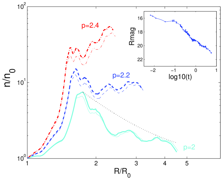
Figure 1: The external density profiles, $n(R)$, that reproduce the R-band light curve, for different values of electrons’ index, $p$: $p=2.4$ (dashed-doted), $p=2.2$ (dashed line) and $p=2$ (solid line). The thick lines are the exact numeric solution of Eqs. 8-10. The thin lines are the analytic solution of Eq. 12. The thin dotted line depicts the expected amplitude of the density fluctuations, $\Delta n(R)\propto R^{-5/2}$, for a random distribution of clumps inside a uniform density background, $n_{0}$. The normalization is derived assuming that the first bump is due to a single clump. The inset on the right depicts the R-band observed data points and the fitted light curve. The observed R-band data points are taken from: Fox 2002, Uemura et. al. 2002, Oksanen & Aho 2002, Rhoads et. al. 2002, Winn et. al. 2002, Zharikov et. al. 2002, Halpern et.al. 2002a & 2002b, Balman et. al. 2002, Cool & Schaefer 2002, Holland et. al. 2002a & 2002b, Bersier et. al. 2002, Sahu et. al. 2002, Oksanen et. al. 2003, Matsumoto et.al. 2002, Stanek et. al. 2002, Mirabel et. al. 2002, Masseti et. al. 2002, Barsukova et. al. 2002 , Malesani et. al. 2002, Mirabel et. al. 2002.

So far, we have assumed a spherically symmetric external density profile, $n=n(r)$. This may occur due to a variable stellar wind, but is not expected for an ISM. As we obtain that an underlying constant density profile provides a better fit for GRB 0210004, it is more natural to expect density fluctuations in the form of clumps, rather than being spherically symmetric, in this case. This interpretation requires $p\approx 2$ for which the density at large radii decreases back to its value at $R_{0}$. As the density profile for $p=2$ is not smooth, several density clumps are needed. The first clump should be at $R_{1}\approx 1.5R_{0}$ and with an over-density of factor $\sim 8$. In order to have a similar effect as a spherical density bump, the clump must replace all the emitting material, i.e. its size (radius), $l_{\rm cl}$, must be large enough so that its mass is larger than the swept up mass at that radius within an angle of $\gamma^{-1}$ around the line of sight: $l_{\rm cl}>l_{\rm min}=(n_{0}/n_{\rm cl}4\gamma^{2})^{1/3}R_{1}\approx 0.03R_{1}\approx 10^{16}\;$cm. An upper limit on the size of the clump can be put from the fact that the bump in the light curve decays on a time scale $\Delta t\sim t$. Since $R\propto t^{1/4}$ for an ISM, this implies $l_{\rm cl}<l_{\rm max}=(2^{1/4}-1)R_{1}\approx 0.19R_{1}$ (Lazzati et al. (2002) obtain a similar clump size using different considerations).

Assuming a homogeneous distribution of clumps with the same physical size and over-density, the mean distance between neighboring clumps is $d_{\rm cl}\sim(\pi l_{\rm cl}^{2}R_{1})^{1/3}\approx 4-5\times 10^{16}\;$cm, where the numerical estimate assumes $l_{\rm cl}=l_{\rm min}$, in which case the clumps hold roughly $5\%$ of the volume and $30\%$ of the mass (these are lower limits as $l_{\rm cl}>l_{\rm min}$ would imply larger filling factors). Therefore, soon after the collision with the first clump we expect overlap between pulses from different clumps, where the number of clumps that intersect a given shell with a radius R and angular size $1/\gamma$ is $N_{\rm cl}\sim R^{2}l_{\rm cl}/\gamma^{2}d_{\rm cl}^{3}\propto R^{5}$. Since, on average, the clumps hold a constant fraction of the shell’s mass, a single clump constitute a fraction $\propto R^{-5}$ of the matter at this radius. The total fluctuation in the density would be, therefore, $\propto R^{-5/2}$. This is in a rough agreement with the fluctuations in the density profile we have obtained for p=2 (see Fig 1).

3.2 A Variable Energy Profile

We solve Eqs. 14 and 15 numerically, for a constant ISM density profile, assuming that the energy is constant, $E_{0}$, up to the first observation at $t_{0}$, and letting $E$ vary from this point onwards. Figure 2 depicts the energy profile obtained for different values of $p$ as a function of $\theta=1/\gamma$ (the angular size of the observed area). An electron power law index of $p=2.6$, requires an almost monotonous increase of $E$ in the observed region. Such a profile may arise due to refreshed shocks. However, the continues increase in $E$ requires a continuous arrival of new shells, a scenario which we consider as unlikely. The energy profiles obtained for $p=2.2$ and $p=2.4$ could reflect irregular patches with an initial angular size of $\theta_{\rm fl}\approx 0.02\;$rad and an average energy of several times $E_{0}$. The energy fluctuations decrease with time, as expected from a patchy shell (see Figure 2). The profile obtained for $p=2$ shows an initial rise followed by a gradual (and bumpy) decrease back to the initial value. Such a profile can correspond to a line of sight is $\sim 0.04\;$rad away from a hot spot (the average energy over a large area is $E_{0}$). This hot spot may be a hot patch in an irregular jet. Alternatively, as suggested by Lazzati et al. (2002), this hot spot may be the core of a jet (on the jet axis) in an axisymmetric angle dependent regular jet. According to this interpretation the angular size of the jet’s core is $\theta_{c}\sim 0.02\;$rad, the isotropic equivalent energy outside the core is roughly constant and its value is $\sim 3$ times less than the core’s energy.

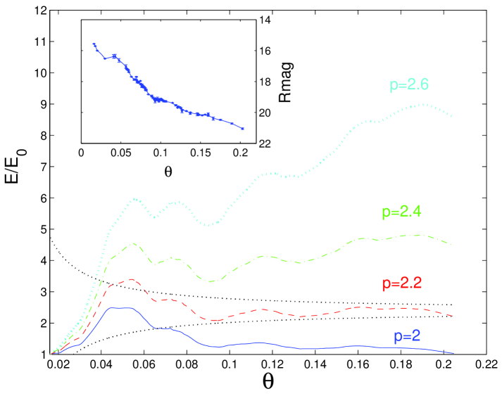
Figure 2: The isotropic equivalent energy, $E$, within an angle $\theta=1/\gamma$ around the line of sight as a function of $\theta$, for different values of $p$: $p=2$ (solid line), $p=2.2$ (dashed line), $p=2.4$ (dashed-dotted line) and $p=2.6$ (bold dotted line). The curves are normalized by the value at the first observation, $E_{0}$. The thin dotted lines outline the expected fluctuations in $E$ for a patchy shell model with fluctuations on an angular scale $\theta_{\rm fl}=0.02$ (using $E=2.4E_{0}\pm 1.9E_{0}(\theta_{\rm fl}/\theta)$). The inset on the left depicts the observed data points as a function of $\theta$ and the fitted curve.

4 Discussion

We have presented general expressions for the afterglow light curve when the energy in the blast wave varies with time and for a variable external density profile. This formalism follows and generalizes the work of SPN98, and relates the variability in the energy and density to the variability in the light curve. Despite the variability in the light curve, the shape of the broad band spectrum remains the same, with some variability in the values of the break frequencies and flux normalization.

We have focused on the slow cooling spectrum at frequencies $\nu>\nu_{m}$, and derived detailed equations for these cases, as they seem the most relevant for the majority of observed optical light curves. Similar equations can be easily derived for other spectral regimes using Eqs. 4-6. We find that for $\nu_{m}<\nu<\nu_{c}$, variability in the light curve can be induced both by variability in the energy or by variability in the external density (or both). A similar behavior is expected for $\nu<\min(\nu_{m},\nu_{c})$, for both slow and fast cooling. For $\nu>\max(\nu_{m},\nu_{c})$ we find that a variable density hardly induces any fluctuations in the light curve, while a variable energy can induce significant fluctuations. We expect a similar behavior for $\nu_{c}<\nu$, in the fast cooling regime.

We applied our formalism to GRB 021004, which displayed significant deviations from a simple power law decay in its optical (R-band) light curve. We find that several different models may provide a reasonable fit to the observed light curve. These include models where the variability is induced either by density fluctuations or by energy fluctuations, where the latter may be caused either by refreshed shocks or by a patchy angular structure of the GRB outflow. These models vary significantly with the value of $p$. Chandra’s observations constrain the electron’s index to be $p=2.2\pm 0.2$, but even under this constrain many different models can produce the observed light curve. A tighter constrain would limit the models considerably. The following models provide a viable fit to the light curve: I) A variable density: a) For $p=2.2$ there is an order of magnitude rise in the density followed by a roughly constant density; b) For $p=2$ we find a similar rise, but then the density gradually decreases back to its initial value; II) A variable energy: a) For $p=2.6$ refreshed shocks are required in order to explain the energy profile; b) For $p\approx 2.2-2.4$ a patchy shell model provides a good fit; c) For $p=2$ a hot spot (possibly the core of an axisymmetric jet) should reside near our line of sight.

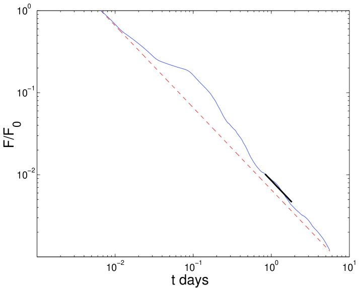
Figure 3: The expected light curve $F_{\nu}(t)/F_{\nu,0}$ for $\nu>{\nu}_{c}$ where $F_{\nu,0}$ is the observed flux at $t_{0}=537\;$sec. The expected light curves are calculated using (i) the energy profile that reproduces the R-band light curve for $p=2$ (solid line) and (ii) the density profile that reproduce the R-band light curve for $p=2$ (dashed line). The short thick line represents Chnadra’s X-ray measurement, normalized for the expected flux at $20.5\;$hr in the varying energy light curve (a power law decay with index $-1$ from $20.5\;$hr till $44\;$hr after the trigger).

As any given single band light curve (which does not show a strong variability on time scales $\Delta t\ll t$) can be reproduced by either density or energy variations, it is important to find ways to distinguish between these two models and their variants. An independently determined value of $p$, say from the spectrum, would have made this task easier (but still not completely determined). Simultaneous light curves both above and below the cooling frequency, $\nu_{c}$, provide the best way to differentiate between a variable energy and a variable density: for the latter strong variability is possible only below $\nu_{c}$. Figure 3 depicts the light curves that are predicted above $\nu_{c}$, using the energy or density profiles deduced from the R-band light curve, that is assumed to be below $\nu_{c}$. Chandra obtained an X-ray light curve between 1 and 2 days (Sako et al. 2002, the thick lines in Figure 3). Unfortunately, by this time the fluctuations expected in the X-ray light curve according to the two models are rather similar and it is hard to distinguish between them. Still, it would be interesting to search for a correlation between the R-band light curve and the X-ray light curve at this time. An earlier X-ray observation could have enabled a clear distinction between the two models.

A variable energy model could arise either from refreshed shocks or from angular inhomogeneity in the jet. In the refreshed socks scenario, we expect during the collision between the two shells an increase in the spectral slope $\beta$ (defined by $F_{\nu}\propto\nu^{\beta}$) and a strong signal in the radio, (Kumar & Piran 2000a). This emission should last over $\Delta t\sim t$. A refreshed shocks can only add energy to the blast wave the total energy in this picture can only increase with time. In the patchy shell model we expect random fluctuations whose amplitude decays with time as $1/\gamma$ (see Fig. 2).

Although the current observations do not enable us to determine which one of the scenarios described above is the correct one (if any), we feel that the patchy shell model with $p=2.2$ (which agrees with the $p=2.2\pm 0.2$ value suggested by Chandra’s observations) is the most likely scenario. According to this interpretation the line of sight of GRB 021004 falls in a “cold spot" where the energy is 2.5 times below the average. This agrees with the observation of rather low $\gamma$-ray flux from this burst. The total $\gamma$-ray energy, $E_{\gamma}=3\cdot 10^{50}\;$ergs is within the standard deviation of the energy distribution presented by Frail et. al (2001), but it is 1.5 times smaller than the average value. On the other hand an extrapolation of Chandra’s measured X-ray flux (Sako et al. 2002) to $11\;$hr after the burst yields $F_{x}\approx 9\cdot 10^{-13}\;{\rm ergs}~{}{\rm cm}^{-2}~{}{\rm sec}^{-1}$. This value is 1.5 times larger than the narrowly clustered value of $F_{x}$ in other bursts: $6\cdot 10^{-13}\;{\rm ergs}~{}{\rm cm}^{-2}~{}{\rm sec}^{-1}$ (Piran et. al. 2001). The X-ray flux reflects $E_{k}$, the kinetic energy of the relativistic ejecta (averaged over an angular scale $1/\gamma$ corresponding to $\gamma\sim 10$). Hence, in this burst $E_{k}/E_{\gamma}$ is larger by a factor of 2.25 than the average value. This factor is similar to the energy fluctuations we find in the patchy shell model for $p=2.2$ (see Fig. 2). While in most GRBs that show a larger value of $E_{k}/E_{\gamma}$ we, most likely, observe a $\gamma$-rays hot spot (Piran 2001). According to this interpretation GRB 021004 is the first burst in which a clear $\gamma$-ray cold spot has been seen.

JG thanks the Hebrew University for hospitality while this research was done. This work was partially supported by the Horwitz foundation (EN) and by the Institute for Advanced Study, funds for natural sciences (JG).

Appendix

Because of the curvature of the afterglow shock, that is spherical rather than planar, photons that are emitted from the shock front at the same time in the source rest frame (i.e. at the same radius), but at different angles from the line of sight, reach the observer at different times. This causes two main effects: first, the bulk of the energy that is emitted at a given time at the source is delayed compared to a photon emitted on the line of sight at that time, and second, at any given time the observer receives photons that were emitted at different radii. In our analysis we take the first effect (angular time delay) into account (see Eq. 3), but the second effect (angular smoothing) is neglected (see Nakar & Piran 2003 for a solution of the spherical symmetric afterglow light curve that takes a full account of the angular effects). For spherical shells, the angular smoothing produces an observed light curve which is a smoothed version of the line of sight emission. The relative importance of angular smoothing is determined by the ratio $t_{\rm los}/t_{\rm ang}$, where $t_{los}=\frac{1}{4c}\int^{R}_{0}dr/\gamma^{2}$ and $t_{\rm ang}\approx R/4c\gamma^{2}$. When the external density decays as a power law, $n\propto r^{-k}$, the line of sight time is: $t_{\rm los}=R/4(4-k)c\gamma^{2}$. Most of the contribution to the observed flux at a time $t_{\rm obs}$, comes from emission at radii $4\lesssim R/ct_{\rm obs}\gamma^{2}(R)\leq 4(4-k)$, which correspond to $t_{\rm los}\leq t_{\rm obs}\lesssim t_{\rm ang}$. Hence, this effect is important when the light curve from the line of sight varies significantly (compared to the smooth power law decay) on time scales shorter than $t_{\rm ang}$ (i.e. $\Delta t_{\rm los}/t_{\rm los}<t_{\rm ang}/t_{\rm los}\sim 4$), which corresponds to density variations on $\Delta R/R\lesssim 0.4$. In such a case the observed light curve is significantly less variable than the line of sight light curve.

We calculate the density profile assuming that the observed (smoothed) light curve is similar to that from the line of sight. Thus, the real density profile has to be more variable than the one we obtain. The difference between the two is smaller when the density profile increases with radius, and the emission along the line of sight increases with time (compared to the power law decay). In this case, the observed flux is dominated by emission from large radii, near the line of sight (with a relatively small contribution from large angles, for which the emission took place at smaller radii, where the external density was relatively low) and the angular smoothing effect is less important. However, when the density drops, the angular effect becomes important. Panaitescu & Kumar (2000) have shown that even a sharp drop in the density produces only a gradual temporal decay in the observed light curve, and that the angular smoothing dictates a maximal power law index of the temporal decay at late times.

The observed R-band light curve of GRB 021004 shows variations on time scales of $\Delta t/t\approx 1<t_{\rm ang}/t_{\rm los}\sim 4$, therefore the angular smoothing effect is not negligible. This effect can be seen by comparing our density profile to the density profile obtained by Lazzati et al. 2002 (their Fig. 1), which take the angular smoothing effect into account. The main difference between the profiles is in the sharp density drop after the first density bump (the density in the profile of Lazzati et al. drops to one order of magnitude below the initial density, while our profile drops back to the initial density). This sharp drop is required, when the angular smoothing is considered, in order to obtain the steep temporal decay in the light curve after the first bump ($t\approx 10^{4}\;$sec).

This last result is obtained under the assumption of a full spherical symmetry. However, it is more likely that the overdense regions are concentrated in clumps and not in spherical shells (see section 3.1 and Lazzati et al. 2002). The radial size of the first clump is $\sim 10^{16}\;{\rm cm}\sim R_{i}/\gamma_{i}$, where $R_{i}$ and $\gamma_{i}$ are the radius and Lorentz factor of the blast-wave when it first interacts with the clump. If we assume that the clump is spherical then its angular size is $\sim 1/\gamma_{i}$ and at the beginning of the first bump ($t\approx 10^{3}\;$sec) it “fills” most of the observed region (the region within an angle of $1/\gamma$ around the line of sight). As the dominant emission is from the hot clump, the angular time remains constant, $R/4\gamma^{2}_{i}$, while $t_{\rm los}$ grows. Therefore, the angular smoothing effect becomes less and less important, and the approximation which neglects this effect holds better than for a spherically symmetric external density profile. Therefore, in this scenario, our method yields a good approximation for the actual density profile at radius $R$, averaged over an angle of $\sim 1/\gamma$ around the line of sight.

References

- [1] \harvarditemBersier D., Winn J., Stanek K.Z. & Garnavich P., 2002, GCN 1586 \harvarditemBalman, S., et al. 2002, GCN 1580 \harvarditemBarsukova E. A., Goranskij, V. P., Beskin G. M., Plokhotnichenko, V. L., & Pozanenko, A. S., 2002, GCN 1606
- [2] \harvarditemBlandford, R. D., & Mckee, C. F., 1976, The physics of Fluids 19, 1130 (1976PhFl...19.1130B)
- [3] \harvarditemChevalier, R. A., & Li, Z., 1999, ApJL, 520, L29 (1999ApJ...520L..29C )
- [4] \harvarditemCool, R. J., & Schaefer, J. J., 2002 GCN 1584 \harvarditemChornock R., & Filippenko A. V., 2002, GCN 1605
- [5] \harvarditemFrail, D. A., et al. 2001, ApJL, 562, L55. (2001ApJ...562L..55F)
- [6] \harvarditemFox D.W., 2002, GCN 1564
- [7] \harvarditemGranot, J., Piran, T., & Sari, R., 1999 ApJ 513, 679 (2000ApJ...534L.163G)
- [8] \harvarditemHalpern, J. P., et al., 2002a, GCN 1578 \harvarditemHalpern, J. P, Mirabal, N., Armstrong, E. K., Espaillat C C.,& Kemp, J., 2002b, GCN 1593 \harvarditemHolland, S., Fynbo, J. P. U., Weidinger, M., Egholm M. P., & Levan, A., 2002a, GCN 1585 \harvarditemHolland, S, et al. 2002b, GCN 1597
- [9] \harvarditemKobayashi, S & Zhang B., to be published in ApJL (astro-ph/0210584)
- [10] \harvarditemKumar, P., & Panaitescu, A., 2000, ApJL 541, L51 (2000ApJ...541L..51K)
- [11] \harvarditemKumar, P., & Granot, J., 2002 submitted to Ap. J.
- [12] \harvarditemKumar, P., & Piran, T., 2000a ApJ, (2000ApJ...532..286K)
- [13] \harvarditemKumar, P.,& Piran, T., 2000b, ApJ, 535, 152 (2000ApJ...535..152K)
- [14] \harvarditemLamb, D., et al. 2002, GCN 1600
- [15] \harvarditemLazzati, D., Rossi E., Covino, S., Ghisellini, G., & Malesani D., 2002 astro-ph/0210333
- [16] \harvarditemMatheson, T., et al. 2002 astro-ph/0210403
- [17] \harvarditemMalesani D., et al., 2002, GCN 1607 \harvarditemMalesani D., et al., 2002, GCN 1645 \harvarditemMasetti N., et al., 2002, GCN 1603 \harvarditemMatsumoto K., et al., 2002, GCN 1594 \harvarditemMirabal N., Armstrong E.K., Halpern J.P. & Kemp J., 2002, GCN 1602 \harvarditemMirabal N., Halpern J.P., Chornock P. & Filippenko A.V., 2002, GCN 1618
- [18] \harvarditemNakar E. & Piran T., 2003, in preperation
- [19] \harvarditemOksanen A. & Aho M., 2002, GCN 1570 \harvarditemOksanen A., et al. 2002, GCN 1591 \harvarditemPiran2001P01Piran, T., Proceedings of the Jan van Paradijs Memorial Symposium "From X-ray Binaries to Gamma Ray Bursts", June 6-8 Amsterdam, eds. E.P.J. van den Heuvel, L. Kaper and E. Rol; Astronomical Society of the Pacific, astro-ph/0111314
- [20] \harvarditemPiran, T., Kumar, P., Panaitescu, A., & Piro, L. 2001, ApJL, 560, L167 (2001ApJ...560L.167P)
- [21] \harvarditemRhoads et al., 2002, GCN 1573 \harvarditemSahu D.K., Bhatt B.C., Anupama G.C. & Prabhu T.P., 2002, GCN 1587 \harvarditemSako M. & Harrison F.A., 2002, GCN 1624 \harvarditemStanek K.Z., Bersier D. & Winn J., 2002, GCN 1598 \harvarditemUemura M., Ishioka R., Kato T. & Yamaoka H., 2002, GCN 1566
- [22] \harvarditemSari, R., Piran, T., & Narayan, R., 1998, ApJL, 497, L17 (1998ApJ...497L..17S)
- [23] \harvarditemWijers, R.A.M.J. 2001, in Gamma-Ray Bursts in the afterglow era, Rome 2000, p.307
- [24] \harvarditemWinn J., Bersier D., Stanek K.Z., Garnavich P. & Walker A., 2002, GCN 1576 \harvarditemZharikov S., Vazquez R. & Benitez G., 2002, GCN 1577
- [25]