Study of a Strategy for Parallax Microlensing Detection Towards the Magellanic Clouds

In this article, we have investigated the possibility to distinguish between different galactic models through the microlensing parallax studies. We show that a systematic search for parallax effects can be done using the currently running alert systems and complementary photometric telescopes, to distinguish between different lens distance distributions. We have considered two galactic dark compact objects distributions, with total optical depths corresponding to the EROS current upper limits. These models correspond to two extreme hypothesis on a three component galactic structure made of a thin disk, a thick disk, and a spherically symmetric halo. Our study shows that for sub-solar mass lenses, an exposure of $8\times 10^{7}$ star$\times$yr toward LMC should allow to distinguish between these two extreme models. In addition the self-lensing hypothesis (lensing by LMC objects) can efficiently be tested through the method proposed here.

1 Introduction

Following the suggestion of Paczyński (Paczyński (1986)), several microlensing surveys are underway to search for dark matter in the form of Massive Compact Halo Objects (MACHO’s). Towards the Magellanic Clouds, 13 to 17 microlensing candidates (depending on the quality) have been found by the MACHO collaboration (Alcock et al. (2000)), 3 candidates were found by the EROS team towards the LMC (Lasserre et al. (2000)) and one towards the SMC (Palanque-Delabrouille et al (1998)). The OGLE collaboration (Udalski et al (1997)) also reported one event towards the LMC.
One of the critical issues concerning the galactic dark matter problem is the localization of the deflecting objects. One way to obtain more information about the location of the lenses is to measure the shape of the light curve with a precision allowing the detection of second order effects. Amongst those effects, the possible use of the well controlled Parallax effect was discussed by (Grieger et al (1986)) and (Gould (1992)). Parallax effect has also been studied towards the galactic bulge by (Buchalter and Kamionkowski (1997)) and LMC by (Gould (1998)). Few parallax microlensing has been observed up to now (Alcock et al. (1995); Mao (1999); Soszyński et al (2001)). However the non-observation of the effect has sometimes been used to put constraints on the parameters of the lens (Palanque-Delabrouille et al (1998), Derue et al. (1999)). In order to increase the sensitivity to the parallax effect, an accurate photometry and a high sampling rate are necessary. One of the ways to reach this aim is to exploit the alert systems of the microlensing surveys with a follow-up setup. EROS is one of the groups that is using an alert system to trigger ongoing microlensing events. The aim of the work presented here is to simulate the observation of microlensing alerts triggered by EROS with a follow-up telescope, and to estimate the efficiency of such a combination to detect the parallax effects. In Section 2, we review the characteristics of parallax distorted events. In Section 3, we present the strategy implemented in our simulation, according to realistic conditions of observation, and we discuss the fitting procedures to the light curves. In Section 4, we give the efficiency of parallax detection and the number of expected parallax events for two extreme galactic models. These results are then discussed in section 5.

2 Parallax Microlensing Events

2.1 Simple Microlensing

So-called standard or simple microlensing events occur when the approximation of a point-like deflector and point-like source with a relative uniform motion is valid. At a given time $t$, the light magnification $A(t)$ of a pointlike source located at distance $D_{s}$ induced by a pointlike deflector of mass $M$ located at distance $xD_{s}$ is given by:

$$A(t)=\frac{{u(t)}^{2}+2}{u(t)\sqrt{4+{u(t)}^{2}}}$$ (1)

where $u(t)$ is the distance between the undeflected line of sight and the deflecting object, expressed in units of the “Einstein Radius” $R_{E}$, the characteristic length of the phenomenon:

$$R_{E} =\sqrt{\frac{4GM}{c^{2}}D_{s}x(1-x)},$$

$$\simeq \ 4.5\ A.U.\times\left[\frac{M_{D}}{M_{\odot}}\right]^{\frac{1}{2}}\times\left[\frac{D_{s}}{10\ Kpc}\right]^{\frac{1}{2}}\times\frac{\left[x(1-x)\right]^{\frac{1}{2}}}{0.5}.$$

Here $G$ is the Newtonian gravitational constant. Assuming a deflector moving at a constant relative transverse speed $v_{T}$, reaching its minimum distance (minimum impact parameter) to the undeflected line of sight $u_{0}$ at time $t_{0}$, $u(t)$ is given by

$$u(t)=\sqrt{{u_{0}}^{2}+(\frac{t-t_{0}}{t_{E}})^{2}},\ where\ t_{E}=\frac{R_{E}}{v_{T}}$$

the “lensing time scale” is the only measurable parameter bringing useful information on the deflector in the approximation of the simple microlensing. Within this approximation, the light curve of a microlensed star with base flux $F_{b}$ is fully determined by the 4 parameters $F_{b},u_{0},t_{0},t_{E}$.

2.2 Parallax Effect in Microlensing

If the variation of the Earth’s velocity rotating component around the sun is not negligible with respect to the projected transverse speed of the deflector, then the apparent trajectory of the deflector with respect to the line of sight is a cycloid instead of a straight line. The resulting amplification versus time curve is therefore affected by this parallax effect. This effect is more easily observable for long duration events (several months), for which the change in the Earth velocity is important (Alcock et al. (1995)). If ${\bf u_{D}(t)}$ is the position of the deflector in the deflector’s transverse plane and ${\bf u_{E}(t)}$ is the intercept of the Earth-source line of sight with this plane (see Fig. 1) , then

$${u(t)}^{2}=|{\bf u_{D}(t)}-{\bf u_{E}(t)}|^{2}.$$ (3)

${\bf u_{D}(t)}$ is given by:

$${\bf u_{D}(t)} = (\frac{t-t_{0}}{t_{E}}cos(\theta)-u_{0}sin(\theta)){\bf i}$$ (4)

$$+ (\frac{t-t_{0}}{t_{E}}sin(\theta)+u_{0}cos(\theta)){\bf j},$$

where $\theta$ is the angle between the projected lens trajectory and the projected major axis of the Earth orbit in the deflector’s plane, $t_{0}$ is the time of the closest approach $u_{0}$ of the lens to the sun-source line of sight, and $t_{E}$ is the Einstein radius crossing time when neglecting the Earth motion (see Fig. 1).

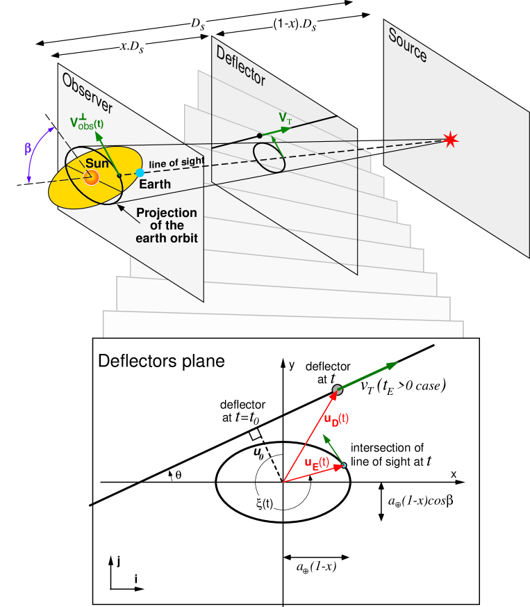
Figure 1: Principle of the parallax effect, and notations used in the text. Here, the lensing configuration is drawn in a referential where the Sun-source line is at rest. Note that changing the sign of $t_{E}$ changes the direction of the deflectors speed. This would have no impact if parallax is neglected.

Here we have chosen the convention to consider negative values of $t_{E}$, which mathematically describe the configurations where the direction of the deflector’s kinetic momentum ${\bf u_{D}(t)}\wedge{\bf v_{T}}$ is inverted, in order to span every possible configuration. Neglecting the earth orbital excentricity, ${\bf u_{E}(t)}$ is given by:

$${\bf u_{E}(t)}=\delta u\ sin(\xi(t)){\bf i}+\delta u\ cos(\xi(t))cos(\beta){\bf j},$$ (5)

where $\delta u=a_{\oplus}(1-x)/R_{E}$ is the projection of the earth orbital radius in the deflector plane in unit of Einstein radius, $\beta$ is the angle between the ecliptic and deflector plane and $\xi(t)$ is the phase of the earth relative to its position when ${\bf u_{E}}=\delta u\ cos(\beta){\bf j}$. The distortion of the light curve is important if the Earth’s orbital velocity around the sun is not negligible with respect to the projected transverse speed of the deflector

$$\tilde{v}=\frac{R_{E}}{t_{E}(1-x)}=\frac{a_{\oplus}}{\delta u.t_{E}}.$$

3 Simulation of a systematic search for parallax

To study the response of the proposed combination of a trigger system with dedicated follow-up capabilities, we have developed a Monte-Carlo simulation of events with parallax effects. In this section, we describe the generation of the event parameters, the EROS trigger system response and the simulation of the expected highly sampled light-curves provided by the follow-up telescope. We then describe a fitting procedure from which we estimate the parallax and its significance for each event. Detection efficiency functions are obtained, which can be combined with any spatial distribution of lenses.

3.1 Simulation of the microlensing events

As mentioned above, simple microlensing light curve depends on 4 parameters, namely the base flux $F_{b}$, $u_{0}$, $t_{E}$ and $t_{0}$. To take into account the parallax, two extra parameters $\theta$ and $\delta u$ need to be generated. The direction of the target, on which depend $\xi(t_{0})$ and $\beta$ should also be fixed. To calculate an efficiency function with uniform statistical precision we generate uniformly the following parameters in their respective intervals: $u_{0}\in[0,2]$, $\log(|t_{E}\,\mathrm{(days)}|)\in[0.7,2.6]$ (positive and negative values for $t_{E}$), $t_{0}\in[t_{first}-50,t_{last}+50]\,\mathrm{(days)}$ where $t_{first}=50$ and $t_{last}=750$, $\theta\in[0,2\pi]$ and $\delta u\in[0,10]$.

3.2 Simulation of EROS-like light curves

The generated parameters of a microlensing event together with the coordinates of the lensed object allows us to write the analytical expression of the magnification versus the time. We keep only the events with $A_{Max}>1.34$. The base fluxes $F_{b}$ of the lensed stars are chosen according to the observed distributions in the EROS catalogues towards LMC and SMC. Light curves are simulated by using the effective sampling rate of EROS towards LMC and SMC (about one observation per six nights in average). Every measurement is then randomly shifted according to a Gaussian distribution that reflects the photometric uncertainties. The average relative photometric precision $\Delta F/F$ for a given flux $F$ (in ADU unit) is taken from the EROS phenomenological parametrisation found for a standard quality image (Derue 1999a ):

$$\frac{\Delta F}{F}=3.5\times F^{-0.85},$$ (6)

3.3 Simulation of a simple alert system

The next step is to simulate an alert system for ongoing events, which is necessary to trigger follow-up observations. According to one of the EROS alert algorithms,we consider that we will monitor events as soon as their light curves exhibit 4 consecutive flux measurements above 4 standard deviations from the base line (Mansoux (1997)). It is clear that only the most significant microlensing events are selected by this algorithm. We have in fact considered several trigger thresholds, from a loose criterion (3 consecutive measurements above $3\sigma$ from the base line) to the strict criterion we finally use. Even using this strict criterion, an average of one false alarm due to variable stars or instrumental artifacts is expected per true microlensing alert (Glicenstein (2002)). This false alarm rate will induce some wasted follow-up time, but for very limited durations, as non-microlensing events would be identified quickly. Figure 2 shows the trigger efficiency as a function of the parallax parameter $Log_{10}(\tilde{v}/30\,\mathrm{km.s^{-1}})$ and the event duration $Log_{10}(t_{E}/1.\,\mathrm{day})$, averaged over all the other parameters. This efficiency is relative to the events for which the earth enters the projected Einstein radius $R_{E}$, i.e. for events with maximum magnification $A_{max}$ larger than 1.34. Note that in the case of strong parallax effect, due to the non-linear trajectory of the earth, this definition may considerably differ from the usual definition of the efficiency relative to events with impact parameter $u_{0}<1$. More details about the efficiency of this algorithm can be found in (Rahvar (2001)).

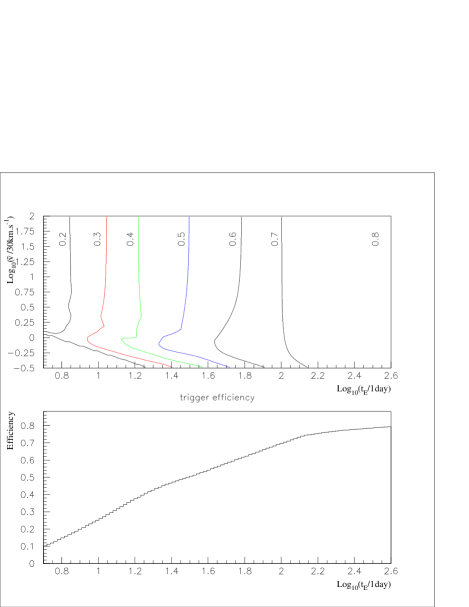
Figure 2: The efficiency of the alert procedure in the $Log_{10}(\tilde{v}/30\,\mathrm{km.s^{-1}})$ vs $Log_{10}(t_{E}/1.\,\mathrm{day})$ plane, for 700 days of observation towards the Magellanic Clouds. This efficiency is the ratio of the number of events that satisfy the trigger conditions, to the number of events – generated with any $u_{0}$ and any date of peak magnification within the $700\pm 50$ days period – with maximum magnification $A_{max}>1.34$. The average efficiency as a function of $Log_{10}(t_{E}/1.\,\mathrm{day})$ is also shown. At this stage, $Log_{10}(\tilde{v}/30\,\mathrm{km.s^{-1}})$ cannot always been experimentally measured.

We assume that the subsequent monitoring of the on-going microlensing events will be made with a telescope large enough to achieve a 1% precision photometry. We also assume that the light curves will be measured two times every night during which the observability of the source exceeds 3 hours, and one time during the other nights. The probability of good weather is taken as $70\%$. We simulate light curves accordingly to these conditions for one colour. Figure 3 shows an example of the simulated light curve including the pre-alert EROS-like measurements and the more precise post-alert measurements.

3.4 Fitting Procedure

After simulating an event that has triggered follow-up observations, we want to estimate the sensitivity to the parallax effect. To this aim, we use a $\chi^{2}$ minimization procedure to reconstruct the 6 microlensing parameters with their errors. Figure 3 allows one to compare the results of this parallax fitting procedure (6 parameters) with a fit that neglects the parallax (4 parameters). In this spectacular example, the $\chi^{2}$ of the best parallax fit is smaller by 2750 units than the $\chi^{2}$ of the best non-parallax fit (for only 2 extra parameters). In the following, we will consider the significance of a parallax signal in units of standard deviation from zero.

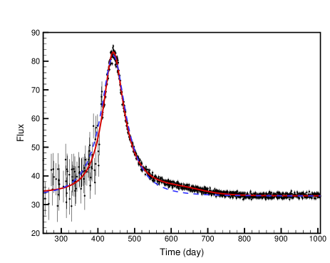
Figure 3: Simulated long timescale microlensing event with $2\%$ photometric precision (flux is in arbitrary units). Pre-alert measurements are affected by much larger error bars (about 10%). The full line corresponds to the parallax fit ($\chi^{2}=1318./(994\,\mathrm{d.o.f})$) and the dashed line corresponds to the Standard fit ($\chi^{2}=4068/(996\,\mathrm{d.o.f})$).

4 Detection of parallax events

The probability to detect a parallax effect not only depends on the 6 parameters that describe a microlensing light curve, but also on the direction of the lensed source as mentioned in sect. 3.1. In practice, we found that the relative change of the average efficiencies from SMC to LMC can be neglected. Figure 4 shows the efficiencies for detecting a parallax effect towards the LMC with $3\sigma$ signification in the $Log_{10}(\tilde{v}/30\,\mathrm{km.s^{-1}})$ versus $Log_{10}(t_{E}/1.\,\mathrm{day})$ plane; these efficiencies are averaged over the parameters that do not depend on the lens population, i.e. the source luminosity, the impact parameter, the date of maximum and the orientation of the lens velocity (assumed to be uniformly distributed from 0. to $2\pi$). This 2-dimensional efficiency function can then be used to estimate numbers of events from any model of the lens population that predicts a $Log_{10}(\tilde{v}/30\,\mathrm{km.s^{-1}})$ versus $Log_{10}(t_{E}/1.\,\mathrm{day})$ distribution.

We have checked that the ratio between significant parallax events and triggered events is almost independent of the trigger threshold. This will allow us to use the concept of relative efficiency to detect parallax events with respect to triggered events $\epsilon_{par}$. We thus assume that the global efficiency $\epsilon_{glob}$ can be written as the product of two terms:

$$\epsilon_{glob}=\epsilon_{trig}\times\epsilon_{par}.$$

Then, in the future, we will be able to obtain realistic numbers by using this relative efficiency with observed rates of events that relates to an effective trigger. As expected, the efficiency to detect a parallax event increases with its duration.

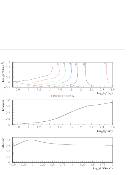
Figure 4: Efficiency of the parallax detection towards the Magellanic Clouds, as a function of $Log_{10}(\tilde{v}/30\,\mathrm{km.s^{-1}})$ vs $Log_{10}(t_{E}/1.\,\mathrm{day})$ (top), as a function of $Log_{10}(t_{E}/1.\,\mathrm{day})$ averaged on $\tilde{v}$ (middle), and as a function of $Log_{10}(\tilde{v}/30\,\mathrm{km.s^{-1}})$, averaged on $t_{E}$ (bottom). Here we assume a photometric follow-up precision of $1\%$ after the alert detection. The efficiency is the ratio of the number of simulated events satisfying the parallax detection conditions, to the number of events generated with any $u_{0}$ and any date of peak magnification within the $700\pm 50$ days period, and with $A_{max}>1.34$.

4.1 Parallax detection and Galactic Models

We have produced theoretical $Log_{10}(\tilde{v}/30\,\mathrm{km.s^{-1}})$ versus $Log_{10}(t_{E}/1.\,\mathrm{day})$ distributions of microlensing events towards the ${\it LMC}$ and ${\it SMC}$, for two extreme models. The first model (model 1) has a “thin” disk completely made of compact objects, with a standard isotropic and isothermal halo including a maximum fraction of compact objects that is compatible with the published EROS limits (Lasserre et al. (2000)). The second model (model 2) has a “thin” plus a “thick” disks both completely made of compact objects, and a very light halo including a maximum fraction of compact objects given by the EROS limits published in (Lasserre (2000)).

• Halos

  The maximum contribution of compact objects in a halo – compatible with the EROS data – depends on its mass function; we consider here 4 different halo mass functions, namely Dirac distributions peaked at $10^{-2}$,$10^{-1}$,$1.$ and $10.M_{\odot}$ respectively. The corresponding maximum fractions of compact objects, that we use in our simulation, are given in table 1 for the two haloes considered here.

  Table 1: Maximum relative contribution of deflectors to the standard and light halos (from Lasserre et al. (2000) & Lasserre (2000).

  	model 1	model 2
  Mass of deflectors	standard halo	light halo
  $10^{-2}M_{\odot}$	13%	23%
  $10^{-1}M_{\odot}$	20%	37%
  $1.M_{\odot}$	36%	87%
  $10.M_{\odot}$	80%	100%

  The so-called standard Halo model has a spherical density distribution $\rho(R)$ given by Caldwell and Coulson (1986):

  $$\rho_{H}(R)=\rho_{H\odot}\frac{{{R_{c}}^{2}+R_{\odot}}^{2}}{R^{2}+{R_{c}}^{2}},$$ (7)

  where $\rho_{H\odot}$ is the local halo density, $R_{c}$ is the halo “core radius” and $R_{\odot}=8.5\,\mathrm{kpc}$ is the Sun distance from the Galactic Centre.

  The light halo model has a density distribution of a spherical Evans type halo (Evans (1994)) given by:

  $$\rho_{H}(R)=\frac{V_{a}^{2}}{4\pi G}\frac{R^{2}+3R_{c}^{2}}{(R^{2}+R_{c}^{2})^{2}}$$ (8)

  where the asymptotic velocity $V_{a}=170\,\mathrm{km/s}$ and G is the Newtonian gravitational constant. Velocities of halo objects follow the Maxwell-Boltzmann distribution with a dispersion of $\sim 200\,\mathrm{km/s}$. The observer and source motions can be neglected when considering the transverse velocity with respect to the line of sight.

• Disks

  The mass functions of disks populations are taken from Gould et al (1997) for the two disks. The density distribution in a disk is modeled in cylindrical coordinates by a double exponential:

  $$\rho_{D}(r,z)=\frac{\Sigma}{2H}\exp\left(\frac{-(r-R_{\odot})}{R_{d}}\right)\exp\left(\frac{-|z|}{H}\right)\ ,$$

  where $\Sigma$ is the column density of the disk at the Sun position, $H$ the height scale and $R_{d}$ the length scale of the disk. The distribution of the lens transverse velocity with respect to the line of sight is established from the sun’s proper motion within the thin disk and from the local velocity distributions of the disk objects described by the dispersion ellipsoids with $\sigma_{r},\ \sigma_{\theta},\ \sigma_{z}$ dispersions; the eventuality of a significant vertical gradient for the thick disk rotation velocity is still a matter of debate. At $1\,\mathrm{kpc}$ from the Galactic plane (mean distance of the thick-disk lenses), estimates of the average differential velocity between the thick and the thin disks vary from $0$ to $-30\,\mathrm{km/s}$ (Beers and Chiba (2001), Binney and Merrifield (1998)). As long as this constant term is smaller than $\sigma_{r}$, its impact on the transverse speed distribution can be neglected. Otherwise, the microlensing events would be shorter and the distributions discussed below would be distorted accordingly. In the case of lensing by a disk object, we neglect the source proper motion, because of its much larger distance.

The model parameters we use in this paper are summarized in Table 2.

Table 2: Parameters of the galactic models used in this article and predictions of the rotation curve of the Milky Way.

Structure	Parameter		model 1	model 2
	$\Sigma\ (M_{\odot}\,{\rm pc}^{-2})$		50
	$H\ ({\rm kpc})$		0.325
Thin	$R_{d}\ ({\rm kpc})$		3.5
disk	$M_{thin}(\times 10^{10}M_{\odot})$		4.4
	velocity	$\sigma_{r}\ \mathrm{(km/s)}$	34.
	disper-	$\sigma_{\theta}\ \mathrm{(km/s)}$	28.
	sions	$\sigma_{z}\ \mathrm{(km/s)}$	20.
	$\Sigma\ (M_{\odot}\,{\rm pc}^{-2})$		-	30
	$H\ ({\rm kpc})$		-	1.0
Thick	$R_{d}\ ({\rm kpc})$		-	3.0
disk	$M_{thick}\ (\times 10^{10}M_{\odot})$		-	2.9
	velocity	$\sigma_{r}\ \mathrm{(km/s)}$	-	51.
	disper-	$\sigma_{\theta}\ \mathrm{(km/s)}$	-	38.
	sions	$\sigma_{z}\ \mathrm{(km/s)}$	-	35.
	$\rho_{H\odot}\ (M_{\odot}\,{\rm pc}^{-3})$		0.008	0.005
Halo	$R_{c}\ ({\rm kpc})$		5.0	15.0
	$M\ {\rm in}\ 60\,{\rm kpc}\ (10^{10}M_{\odot})$		51	22
	velocity	$\sigma$ (km/s)	200.	200.
	$\rho_{\odot}\ (M_{\odot}\,{\rm pc}^{-3})$		0.085	0.097
Predictions	$V_{rot}\ {\rm at}\ {\rm sun}\ ({\rm km}\,{\rm s}^{-1})$		192	219
	$V_{rot}\ {\rm at}\ 50\,{\rm kpc}$		199	182

Figures 5 and 6 show the expected distributions of events towards LMC, for the two Galactic models and the 4 halo mass functions, respectively peaked at $10^{-2}$, $10^{-1}$, 1. and $10.M_{\odot}$.

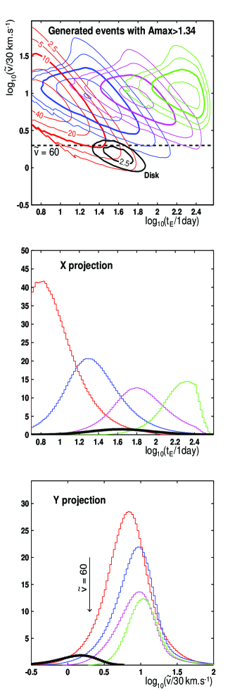
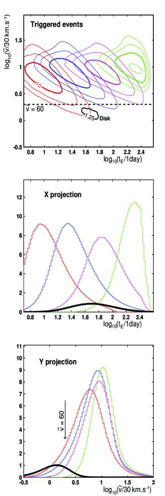
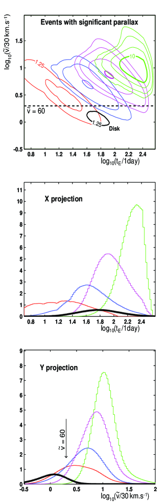
Figure 5: Expected distributions of microlensing events in the $Log_{10}(\tilde{v}/30\,\mathrm{km.s^{-1}})$ versus $Log_{10}(t_{E}/1.\,\mathrm{day})$ plane and projections for the various components of model 1. The maximum contributions of halo objects of $10^{-2}$, $10^{-1}$, $1.$ and $10.M_{\odot}$, compatible with the observed microlensing rates, are respectively plotted in each 2D frame from left to right. The thin disk contribution lies in the lower part of the 2D frames.
-Left panels: events with $A_{max}>1.34$.
-Center: events that satisfy the trigger requirements.
-Right: events that exhibits a $3\sigma$ significant parallax.
The iso-density contour levels follow a geometrical series: the difference between consecutive levels of density is a factor 2. The thick contours always correspond to 10 events per abscissa unit and per ordinate unit, for an exposure of $E=1\,\mathrm{year}\times 10^{7}\,\mathrm{stars}$. For clarity of the figure, different scales (explicitely indicated) may be used for the disk contributions. The vertical scales for the projections give the expected numbers of events per abscissa unit, for an exposure of $E=1\,\mathrm{year}\times 10^{7}\,\mathrm{stars}$.

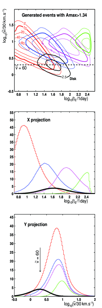
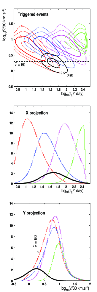
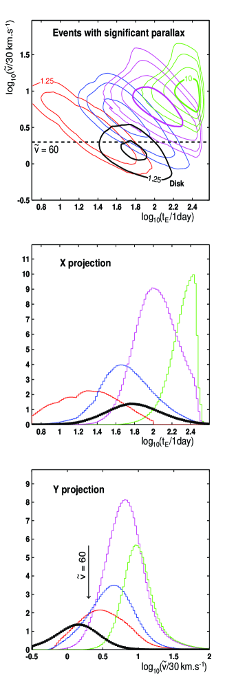
Figure 6: Expected distributions of microlensing events for model 2 (see caption of Fig. 5). The thin plus thick disk contributions lie in the lower part of the frames.

The choice of $\tilde{v}$ and $t_{E}$ gives to these distributions some interesting scaling features because $\tilde{v}$ is a projected speed that only depends on the position and velocity of the deflector (not on its mass), and $t_{E}$ scales with $\sqrt{M_{deflector}}$ for a given spatial and velocity distribution. Then, for a fixed spatial and velocity distribution of the compact halo objects, we can predict the scaling of the $Log_{10}(\tilde{v}/30\,\mathrm{km.s^{-1}})$ versus $Log_{10}(t_{E}/1.\,\mathrm{day})$ distribution when changing the mass function, assuming that no experimental bias is introduced (i.e. before any selection process); we expect this initial (unbiased) $Log_{10}(\tilde{v}/30\,\mathrm{km.s^{-1}})$ versus $Log_{10}(t_{E}/1.\,\mathrm{day})$ distribution to be simply horizontally translated by +0.5 unit when the mass of the deflectors is multiplied by 10; the integral of the distribution should also be scaled by $1/\sqrt{10}$ times the corresponding fraction of the halo made of such compact objects.

The left panels of figures 5 and 6 reflect these properties, with limitations due to truncations in $t_{E}$. It also appears that the general shape of the halo distribution is almost unaffected by the choice of a standard or light halo. The trigger and parallax detection efficiencies distort considerably these distributions.

5 Discussion

We center the discussion on the LMC case, considering its larger rate of detectable events compared to the SMC case. Anyway, as already mentioned in Sect. 4, the efficiency diagrams can also be used as it for the SMC studies. The halo mass function is mainly bounded by the upper limit established for each mass by the microlensing surveys, but its actual shape is unknown. Then, a given observed microlensing $t_{E}$ distribution can generally be explained by the two halo models; indeed, for each halo, appropriate mass function shapes (i.e. not anymore simple delta functions) can be found which, added to the disk(s) contribution(s), satisfy our published upper limits, and result in identical microlensing $t_{E}$ distributions. Our proposed strategy provides a sensitivity to the parallax effect that allows to distinguish the self-lensing and the halo contributions from the disk(s) one(s), and also to remove the degeneracy between our 2 models. Table 3 gives the rates of events expected to trigger complementary observations, the rates of events with a $3\sigma$ significant parallax and with $\tilde{v}<60\,\mathrm{km/s}$, and the ratios of the parallax events to the trigger events, assuming 1% photometric precision after the alert. As mentioned before, these ratios are unsensitive to the effective trigger threshold, and can be used with the effective observed alert rate.

Table 3: Rates of parallax events and ratios to trigger events (in %), assuming 1% photometric precision, for an exposure of $1\,\mathrm{year}\times 10^{7}\,\mathrm{stars}$.

Mass of	Trigger	with detected	with
halo lenses	events	parallax $>3\sigma$	$\tilde{v}<60\,\mathrm{km/s}$
model 1 - standard halo, thin disk
$10^{-2}M_{\odot}$	4.9	0.92 (19%)	0.14 (2.8%)
$10^{-1}M_{\odot}$	6.5	2.0 (31%)	0.28 (4.3%)
$1.M_{\odot}$	5.4	3.4 (63%)	0.09 (1.7%)
$10.M_{\odot}$	4.9	4.0 (82%)	0. (0.%)
thin disk	0.7	0.42 (62%)	0.36 (53%)
model 2 - light halo, thin+thick disks
$10^{-2}M_{\odot}$	8.3	1.9 (23%)	0.54 (6.5%)
$10^{-1}M_{\odot}$	7.1	2.7 (39%)	0.44 (6.2%)
$1.M_{\odot}$	7.6	5.3 (71%)	0.16 (2.1%)
$10.M_{\odot}$	3.4	2.9 (84%)	0. (0.%)
thin+thick disks	1.7	1.0 (59%)	0.7 (41%)

From this table, we can conclude that requesting for a strong parallax effect (with $\tilde{v}<60\,\mathrm{km/s}$) essentially selects disks events, due to the proximity of their lensing objects.

• If the disk contribution to the microlensing signal is dominant (no compact objects in the halo), then about half of the events will exhibit a parallax deviation with $\tilde{v}<60\,\mathrm{km/s}$

• If the halo contribution is important, then the fraction of events with $\tilde{v}<60\,\mathrm{km/s}$ will be much smaller.

• If the so-called “self-lensing” contribution is dominant, then this fraction will be negligible. The self-lensing hypothesis assumes that the microlensing events are due to lenses belonging to the LMC or the SMC. Such events would never give a detectable parallax effect, and our simulation shows that they would lie above the upper part of the $Log_{10}(\tilde{v}/30\,\mathrm{km.s^{-1}})$ versus $Log_{10}(t_{E}/1.\,\mathrm{day})$ diagram of figures 5 and 6.

5.1 Distinguishing between the halo models

Figure 7 gives for the 2 models the rate of events that exhibit a significant parallax effect ($>3\sigma$), and the rate of events with a projected speed $\tilde{v}<60\,\mathrm{km/s}$, as a function of the halos deflectors mass. The $\tilde{v}<60\,\mathrm{km/s}$ cut corresponds to $Log_{10}(\tilde{v}/30\,\mathrm{km.s^{-1}})<0.3$ in figures 5 and 6. The right part of Fig. 7 illustrates the effect of a photometric precision degradation down to 4%: the sensitivity to parallax is typically downgraded by 25%.

Figure 7: Rates of significant parallax events ($>3\sigma$) (upper panels), and of events with $\tilde{v}<60\,\mathrm{km/s}$ (lower panels) as a function of the halos deflectors mass. Thick lines correspond to model 1, thin lines to model 2. The lower (horizontal) lines belong to a null halo contribution, the upper lines belong to the maximum halo contribution of objects with mass indicated by the abscissa. Left panels are calculated for a 1% photometric precision, right panels for a 4% precision. The numbers are given for one year of observation of $10^{7}$ stars in the field of LMC.

From this figure, one can estimate the minimal exposure allowing to separate models that predicts comparable optical depths; we consider that models 1 and 2 with a maximum contribution of halo objects (respectively $\mu_{1}$ and $\mu_{2}$ events expected with $3\sigma$ significance parallax for $10^{7}\,\mathrm{star}\times\,\mathrm{year}$), can be distinguished if the exposure $\alpha\times 10^{7}\,\mathrm{star}\times\,\mathrm{year}$ is large enough to allow a significant separation of the two expected distributions of the events numbers. We choose the convention that the mean values of the two distributions should be separated by at least the sum of their widths. This condition can be expressed as follows:

$$|\alpha\mu_{1}-\alpha\mu_{2}|>\sqrt{\alpha\mu_{1}}+\sqrt{\alpha\mu_{2}}\ \Longrightarrow\alpha>\frac{(\sqrt{\mu_{1}}+\sqrt{\mu_{2}})^{2}}{(\mu_{1}-\mu_{2})^{2}}$$

Figure 8 shows the minimum exposure needed to distinguish between the two models, as a function of the mass of the halo objects.

Figure 8: Minimum exposures needed to discriminate between the two halo models as a function of the mass of the halo objects, in years for $10^{7}$ stars of the LMC. This exposure corresponds to the same number of years of parallax studies with an EROS-type alert system. Notice that this is needed to distinguish between models with the maximum allowed fraction of compact objects. These numbers are based on our simulated trigger efficiency $\epsilon_{trig}$. As mentioned in the beginning of section 4, they may need to be normalised if the true efficiency is very different. The thin line corresponds to 1% photometric precision, the thick line belongs to 4% precision.

A few years of parallax studies with an EROS-type alert system (monitoring $\sim 10^{7}$ stars) are needed to separate the two halo models if the halo objects are lighter than the solar mass. The critical aspect of the photometric precision is clearly visible on the figure. A definitive model separation – taking into account the complete allowed domains for the mass functions – will probably need the extraction of parallax events with $\tilde{v}<60\,\mathrm{km/s}$, specially if there is very few halo events (the most pessimistic case: if the halo fraction made of compact objects is small or if these objects are very heavy). Then, an exposure of several $10^{8}\,\mathrm{star}\times\,\mathrm{year}$ is needed, that should be accessible after a few years of running a next generation microlensing survey. Obviously, more sophisticated analysis, such as likelyhood analysis, should be done after the detection of a reasonable sample of parallax events.

5.2 Self-lensing

If self-lensing is dominant, then very few lenses (only those belonging to the disk) will produce a detectable parallax. The relevant parameter to test this hypothesis will be the ratio of the parallax events to the triggered events. EROS (phase 2) found 2 events for an exposure of $3\times 10^{7}\,\mathrm{star}\times\,\mathrm{year}$ towards the LMC (Lasserre et al. (2000)). If this rate is due to halo and disk objects then, according to Table 3, typically 50% of the events should have a measurable parallax. On the other hand, if the observed events are only due to self-lensing, then none will have a measurable parallax. About 5 years of parallax studies would then be needed to observe or not 2 to 3 parallax events that would allow to discriminate between the two hypothesis.

6 Conclusion and perspectives

In this study, we have investigated a strategy to detect parallax effects in microlensing with an optimal efficiency, through the triggering of follow-up observations. Parallax measurements will allow to distinguish between a nearby population of lenses (belonging to the disks) and a remote population. One of the most interesting outcome of such parallax studies would be to solve the question of the self-lensing hypothesis, which assumes that the microlensing events are mostly due to lenses belonging to the LMC or SMC. A definitive separation between models of lens spatial repartition may need several years of data taking for a new generation of microlensing survey. Such measurements need a high sampling follow-up of the triggered microlensing events towards LMC and SMC, with a 1% photometric precision. A partially dedicated one meter class telescope could achieve this precision through reasonnably long exposures ($\sim 30\,\mathrm{min.}$). Finally, it should be mentioned that such parallax monitoring will also have other applications. A systematic search for source size effects such as saturation of the maximum magnification can be performed from the same data. In favourable cases (small impact parameter events) this would allow to obtain additional constraints on the lens configurations, that are complementary to the ones inferred from parallax analysis.

References

- Alcock et al. (2000) Alcock C., Allsman R.A., Alves D.R. et al 2000, ApJ 542, 281.
- Alcock et al. (1995) Alcock C., Allsman R.A., Alves D. et al 1995, ApJ 454 , L125.
- Aubourg et al. (1993) Aubourg, E. et al 1993, Nature, 365, 625.
- Ansari et al. (1996) Ansari R., Cavalier C., Moniez M. et al 1996, A&A 314, 94.
- Beers and Chiba (2001) Beers T.C., Chiba M., in Astrophysical Ages and Time Scales, ASP Conf. Series, Vol. TBD, 2001, T. von Hippel, N. Manset, C. Simpson.
- Binney and Merrifield (1998) Binney J., Merrifield M., in Galactic Astronomy, 1998, Princeton University Press.
- Buchalter and Kamionkowski (1997) Buchalter, A., Kamionkowski, M. 1997, APJ 482, 782.
- Caldwell and Coulson (1986) Caldwell J., Coulson I. 1986, MNRAS 218, 223.
- (9) Derue F., 1999a, Ph.D. thesis, CNRS/IN2P3, LAL99-14 report.
- Derue et al. (1999) Derue F., Afonso C., Alard C. et al (EROS) 1999, A&A 351, 87.
- Evans (1994) Evans N.W. 1994, MNRAS 267, 333.
- Glicenstein (2002) Glicenstein J-F., 2002, private communication.
- Gould (1992) Gould A., 1992, APJ 392, 442.
- Gould et al (1997) Gould A., Bahcall J.N., Flynn C., 1997, ApJ 482, 913.
- Gould (1998) Gould A., 1998, APJ 506, 253.
- Grieger et al (1986) Grieger, B., Kayser, R., Refsdal, S. 1986, Nature 324, 126.
- Lasserre (2000) Lasserre T., 2000. Ph.D. thesis, CEA, DAPNIA/SPP-00-04-T report.
- Lasserre et al. (2000) Lasserre, T. et al. (EROS) 2000, A&A 355, L39.
- Mansoux (1997) Mansoux B., 1997, Ph.D. thesis, CNRS/IN2P3, LAL report 97–19.
- Mao (1999) Mao, S. 1999, A&A 350, L19.
- Paczyński (1986) Paczyński, B. 1986, ApJ 304, 1.
- Palanque-Delabrouille et al (1998) Palanque-Delabrouille N. et al (EROS), 1998, A&A 332, 1.
- Rahvar (2001) Rahvar, S., 2001, Ph.D. thesis, Sharif University of technology, 04/33491, Tehran, Iran.
- Soszyński et al (2001) Soszyński, I., Zebruń ,K., Woźniak, P.R. et al, 2001, ApJ 552, 731.
-
Udalski et al (1997)
Udalski, A., et al. 1997, Acta Astronomica, 47, 319;
http://www.astrouw.edu.pl ogle/ogle2/ews/ews.html.