Physical properties of two low-luminosity $z\sim 1.9$ galaxies behind the lensing cluster AC 114

We present VLT/ISAAC near-infrared spectroscopy of two gravitationally-lensed $z\sim 1.9$ galaxies, A2 and S2, located behind the cluster AC 114. Thanks to large magnification factors, we have been successful in detecting rest-frame optical emission lines (from [O ii]$\lambda$3727 to $\rm H{\alpha}$+[N ii]$\lambda$6584) in star-forming galaxies 1 to 2 magnitudes fainter than in previous studies of Lyman break galaxies (LBGs) at $z\sim 3$. From the $\rm H{\alpha}$ luminosity, we estimate star formation rates (SFRs) of 30 and 15 M_⊙ yr^-1 for S2 and A2 respectively. These values are 7 to 15 times higher than those inferred from the UV continuum flux at 1500Å without dust extinction correction. In setting SFR_Hα $\sim$ SFR_UV, one derives extinction coefficients E(B-V) $\sim$ 0.3 for S2 and E(B-V) $\sim$ 0.4 for A2. The behavior of S2 and A2 in terms of O/H and N/O abundance ratios are very different, and they are also different from typical LBGs at $z\sim 3$. S2 is a low-metallicity object ($Z\sim$ 0.03 Z_⊙) with a low N/O ratio, similar to those derived in the most metal-poor nearby Hii galaxies. In contrast, A2 is a high-metallicity galaxy ($Z\sim$ 1.3 Z_⊙) with a high N/O abundance ratio, similar to those derived in the most metal-rich starburst nucleus galaxies. The line-of-sight velocity dispersions, derived from emission line widths, are 55 and 105 km s^-1, yielding a virial mass of 0.5 and 2.4 $\times 10^{10}$ M_⊙, for S2 and A2 respectively. Thanks to the gravitational amplification, the line profiles of S2 are spatially resolved, leading to a velocity gradient of $\pm 240$ km s^-1, which yields a dynamical mass of $\sim 1.3\times 10^{10}$ M_⊙ within the inner 1 kpc radius. Combining these new data with the sample of LBGs at $z\sim 3$, including the lensed galaxy MS 1512-cB58, which is the only LBG for which physical properties have been determined with similar accuracy, we conclude that these three galaxies exhibit different physical properties in terms of abundance ratios, SFRs, $M/L_{\rm B}$ and reddening. High-redshift galaxies of different luminosities could thus have quite different star formation histories.

1 Introduction

With the recent advent of near-infrared (NIR) spectrographs on 8-10m class telescopes, a quantitative study of the rest-frame optical properties of high-redshift galaxies is now possible. Indeed, NIR spectroscopy allows one to compare directly the physical properties of high-redshift galaxies (star formation rate, reddening, metallicity, kinematics, virial mass) with galaxies in the local Universe through line-based indicators.

The pioneering work by Pettini et al. (1998, 2001) has shown that the rest-frame optical properties of the brightest Lyman break galaxies (LBGs) at $z\sim 3$ are relatively uniform. However, the sample of LBGs observed in the NIR is small and limited to the brightest examples (Pettini et al. 1998, 2001; Kobulnicky & Koo 2000; Teplitz et al. 2000; Shapley et al. 2001). Additionally, the $1.5\raisebox{-2.15277pt}{$\,\stackrel{{\scriptstyle<}}{{\scriptstyle\sim}}\,$}z\raisebox{-2.15277pt}{$\,\stackrel{{\scriptstyle<}}{{\scriptstyle\sim}}\,$}2.5$ redshift interval remains unexplored because of the lack of strong spectral features that can be used to identify such sources with visible spectrographs.

Massive clusters acting as Gravitational Telescopes (GTs) constitute a powerful tool in the study of high-redshift galaxies. They have been successfully used over a wide range of wavelengths, ranging from the UV to the sub-mm (e.g. Smail et al. 1997; Bézecourt et al. 1999; Ebbels et al. 1998; Pelló et al. 1999; Altieri et al. 1999; Ivison et al. 2000) and allowed recently to detect the most distant galaxies ($z\ga 5$; Ellis et al. 2001; Hu et al. 2002). The large magnification factors of galaxies that are close to the critical lines (typically 1 to 3 magnitudes) can be used to probe the physical properties of intrinsically faint high-redshift galaxies, which would otherwise be beyond the limits of conventional spectroscopy (e.g. Ebbels et al. 1996; Pelló et al. 1999, Mehlert et al. 2001).

Large samples of $z\raisebox{-2.15277pt}{$\,\stackrel{{\scriptstyle>}}{{\scriptstyle\sim}}\,$}2.5$ star-forming galaxies have become available in the recent years, mainly through the Lyman break technique (Steidel et al. 1996, 1999). Our sample of highly-magnified, high-redshift galaxies extends these samples towards intrinsically fainter galaxies, allowing us to probe the physical properties of galaxies that are 1 to 3 magnitudes fainter than the present LBGs studies (Steidel et al. 1996, 1999; Pettini et al. 1998, 2001). The sample has been selected from lensing clusters with well constrained mass distributions, first through photometric redshift and lens-inversion techniques, and later confirmed spectroscopically (e.g. Kneib et al. 1996; Ebbels et al. 1998; Campusano et al. 2001). Lensed galaxies for spectroscopic follow-up are chosen to be close to the high-redshift critical lines in order to obtain the largest magnification (typically $\sim 2$ magnitudes).

In this paper, we present NIR spectroscopy on two high-redshift galaxies ($z\sim 1.9$) that are lensed by the massive cluster AC 114 ($z=0.312$). AC 114 is a rich source of multiply-imaged, high-redshift galaxies (Smail et al. 1995; Natarajan et al. 1998, Campusano et al. 2001). The two lensed galaxies, named S2 and A2 according to Natarajan et al. 1998, correspond to multiple images of two different sources at very similar redshifts. A mass-model, first obtained by Natarajan et al. (1998) and later improved by Campusano et al. (2001), allows us to recover the intrinsic properties of S2 and A2. Thanks to the large magnification of these sources, we have measured for the first time several important emission lines from NIR spectroscopy of high-redshift galaxies fainter than $M_{\rm B}$ = $-21$.

The plan of the paper is as follows. In Sections 2 and 3, we summarize the observations and describe the steps in converting the two dimensional raw data into calibrated one dimensional spectra. Emission-line intensities and FWHMs are presented in Section 4 and analysed in Section 5. Star formation rates, O/H and N/O abundance ratios and kinematics are derived here. In Section 6 these new data are combined with existing samples of LBGs at $z\sim 3$ in order to understand where high-redshift galaxies lie in two fundamental scaling relations: N/O versus O/H abundance ratios and the metallicity–luminosity relation. Finally, the main results of this work are summarized in Section 7. Throughout this paper, we assume a cosmology with $\Omega_{0}=0.3$, $\Lambda=0.7$ and $H_{0}$ = 70 km s^-1 Mpc^-1.

2 Observations

The data were obtained with the NIR spectrograph ISAAC, which is located on the Nasmyth B focus of Antu (VLT-UT1), during UT 2001 September 26-27 (period 67). The data were obtained with the Short-wavelength channel (Cuby et al. 1999), which uses a $1024\times 1024$ Hawaii Rockwell array, and the medium resolution grating. The slit width was 1″.

Because the redshifts and spectral energy distributions (hereafter SED) of the sources in the cluster core were known before the run, we could optimize the use of the grating settings to search for the most relevant spectral features. To cover $\rm H{\alpha}$, $\rm H{\beta}$, [O iii] $\lambda\lambda$4959,5007, and [O ii] $\lambda\lambda$3726,3728, three settings with the ISAAC medium resolution grating were used.

The ISAAC 120″ long slit allowed us to align at least 2 objects per setting in the inner region of the cluster. In the present case, we targeted the two gravitationally amplified sources AC114-S2 and AC114-A2, both of them at redshift $z\sim 1.9$, together with the offset star. Figure 1 shows an HST/WFPC2 image (F702W) of AC114 and the long-slit configuration.

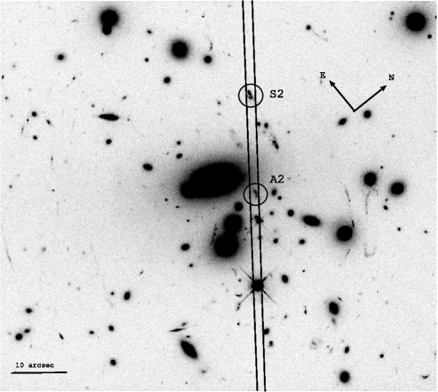
Figure 1: HST/WFPC2 image ($R$-band/F702W) of the core of AC114. The position of the ISAAC slit used in our observations is displayed. Circles mark the position of the high redshift galaxies AC114-S2 and AC114-A2.

Table 1 summarizes the wavelength regions that were selected to contain the redshifted emission lines of [O ii] $\lambda\lambda$3726,3728, [O iii] $\lambda\lambda$4959,5007, $\rm H{\alpha}$, and [N ii] $\lambda$6584. The integration times and the airmasses are also listed.

Table 1: Summary of ISAAC Observations

	[OII]	[OIII]	$\rm H{\alpha}$
Atm. window	$Y$	$H$	$K$
$\lambda$ (Å) observed	10500-10840	13900-14500	18400-19400
$\lambda$ (Å) rest-frame	3662-3780	4848-5057	6417-6766
Exposure (s)	$8\times 900$	$8\times 900$	$8\times 900$

$Y$-band                                             $K$-band

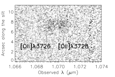
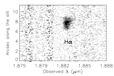
$H$-band

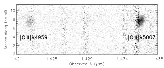
Figure 2: Two-dimensional images of the ISAAC spectra of AC114-S2 in the $Y$ (1.0 to 1.1 $\mu$m), $H$, and $K$ bandpasses. Positions of the nebular emission lines are labeled.

The ISAAC observations were performed in beam-switching mode. The objects were observed at two slit positions, which we label A and B. After an A-B-B-A sequence, the object was re-acquired at a different slit position, and the sequence was repeated. The seeing varied between $\sim 0.5$ and $\sim 1.5$ arcsec and airmass varied between 1.2 and 1.4.

Figure 3: The extracted one-dimensional $Y$, $H$, and $K$ band spectra of AC114$-$S2. The dashed line shows the 1 $\sigma$ error spectrum. Spectra have been smoothed to the instrumental resolution.

Figure 4: The extracted one-dimensional $Y$, $H$, and $K$ band spectra of AC114$-$A2. The dashed line shows the 1 $\sigma$ error spectrum. Spectra have been smoothed to the instrumental resolution.

3 Data reduction and calibration

We used IRAF with reference to the ISAAC Data Reduction Guide to convert the two-dimensional raw data into calibrated one-dimensional spectra. The data are first split into AB pairs, and the first step in the reduction process (the first sky subtraction) is to subtract one frame from another in each pair. This step removes both the zero level offset of the array and the sky emission, and results in images with two spectra, one positive and one negative. After trimming and flat fielding, we applied a two-dimensional wavelength calibration. The wavelength calibration, which was derived from the OH lines (Rousselot et al. 2000), also corrects for slit curvature. The next step, the second sky subtraction, removes any residual sky features remaining after the first sky subtraction. During this process, each image is multiplied by $-1$ and added back to itself after a suitable shift. It results in images that have one positive spectrum and two negative spectra either side of the positive spectrum. The resulting spectra, one for each AB pair, are then combined. As an example, the two dimensional spectrum of S2 is shown in Figure 2. The emission lines [O ii] $\lambda\lambda$3726,3728, [O iii] $\lambda\lambda$4959,5007, and $\rm H{\alpha}$ are all clearly detected.

We extracted a one dimensional spectrum from two-dimensional data without fitting the sky since it would only add noise. Removing telluric lines is done by dividing the object spectrum with that of a telluric standard. The telluric standard was observed with the same instrument setup, immediately after the science targets, and it was reduced in the same way and with the same calibration frames as for the science targets. Since the telluric standards were hot stars, a blackbody curve was used to model the continuum of these standards. The blackbody temperature was fixed according to the spectral type of the star. The accuracy of telluric line removals has been checked by computing the observed [O iii] $\lambda$5007/[O iii] $\lambda$4959 line ratio (see Table 2). For S2, we find [O iii] $\lambda$5007/[O iii] $\lambda$4959 = $2.5\pm 0.4$ which, given the measurement uncertainties, agrees with theoretical value of 2.86 (e.g. Osterbrock 1989). Figures 3 and 4 show the extracted one-dimensional infrared $Y$, $H$, and $K$ band spectra of S2 and A2 respectively.

4 Emission line measurements

The emission lines were fitted with one dimensional Gaussians. The integrated fluxes (or 2$\sigma$ upper limits when appropriate) and velocity widths are listed in Table 2. The intrinsic velocity width of emission lines was corrected for the instrumental profile, which is determined from the width of night-sky lines. The redshifts measured for S2 and A2 are 1.867 and 1.869 respectively. In the case of S2, this value agrees with previous measurements (Smail et al. 1995; Campusano et al. 2001). In the case of A2, there is disagreement between the present secure value and the estimate by Campusano et al. (2001), $z=1.687$. Taking into account the correction due to gravitational lensing, the distance between the two objects is about 4″ on the source plane at $z=1.869$, corresponding to $\sim 34$ kpc with the adopted cosmology. As they have similar redshifts, S2 and A2 are thus very close in the source plane and are probably associated with one another. Given the redshifts of A2 and S2, $\rm H{\beta}$ is not detected because it is heavily obscured by telluric absorption between the $Y$ and $H$ bands.

The lensing model by Campusano et al. (2001) was revised to take into account the correct value for the redshift of A2. The resulting magnification factors, 2.0 magnitudes for S2 and 1.7 magnitudes for A2, are similar to the previous estimates (Campusano et al. 2001) and within the model errors ($\sim 0.1$ magnitudes).

Table 2: Spectral Measurements: Line fluxes and FWHM

Emission Line	AC114-S2	AC114-A2	Comments
[O ii] $\lambda$3726 :
$F(\times 10^{-17}$ ergs s-1 cm-2)	$1.8\pm 0.5$		(1)
FWHM (Å)	$5.4\pm 0.7$		(3)
$\sigma$ = FWHM/2.35 (km s-1)	$65\pm 8$		(3)
[O ii] $\lambda$3728 :		[O ii] $\lambda\lambda$3726,3728 :
$F(\times 10^{-17}$ ergs s-1 cm-2)	$1.9\pm 0.4$	$1.5\pm 0.4$	(1)
FWHM (Å)	$4.2\pm 0.4$	$11.9\pm 1.8$	(3)
$\sigma$ = FWHM/2.35 (km s-1)	$50\pm 5$	$142\pm 22$	(3)
[O iii] $\lambda$4959 :
$F(\times 10^{-17}$ ergs s-1 cm-2)	$3.4\pm 0.4$	$<0.9$ (2)	(1)
FWHM (Å)	$6.9\pm 0.5$	…	(4)
$\sigma$ = FWHM/2.35 (km s-1)	$62\pm 5$	…	(4)
[O iii] $\lambda$5007 :
$F(\times 10^{-17}$ ergs s-1 cm-2)	$8.6\pm 0.4$	$2.5\pm 0.4$	(1)
FWHM (Å)	$6.4\pm 0.2$	$9.5\pm 0.4$	(4)
$\sigma$ = FWHM/2.35 (km s-1)	$57\pm 2$	$84\pm 3$	(4)
$\rm H{\alpha}$
$F(\times 10^{-17}$ ergs s-1 cm-2)	$15.6\pm 0.9$	$7.7\pm 0.8$	(1)
FWHM (Å)	$6.6\pm 0.5$	$18.5\pm 0.9$	(5)
$\sigma$ = FWHM/2.35 (km s-1)	$45\pm 3$	$125\pm 6$	(5)
[N ii] $\lambda$6584 :
$F(\times 10^{-17}$ ergs s-1 cm-2)	$<0.8$ (6)	$3.3\pm 0.4$	(1)
FWHM (Å)	…	$13.6\pm 0.9$	(5)
$\sigma$ = FWHM/2.35 (km s-1)	…	$92\pm 6$	(5)

COMMENTS: (1) Measurement by Gaussian fit, corrected for the gravitational magnification factor of 6.31 for AC114-S2 and 4.79 for AC114-A2. (2) Assuming $F_{5007}/2.9$. (3) Intrinsic FWHM after correction for the instrumental profile, modeled as a Gaussian with FWHM=2.3Å. (4) Intrinsic FWHM after correction for the instrumental profile, modeled as a Gaussian with FWHM=4.3Å. (5) Intrinsic FWHM after correction for the instrumental profile, modeled as a Gaussian with FWHM=6.8Å. (6) $2\sigma$ upper limit.

5 Analysis

5.1 Star formation rates

We have compared the star formation rate (SFR) obtained from the UV continuum flux with the value derived from the $\rm H{\alpha}$ emission line, which is the indicator used for galaxies in the local Universe (e.g. Gallego et al. 1995). The rest-frame 1500Å flux for S2 and A2 has been derived from the UV rest-frame FORS1 spectra obtained by Campusano et al. (2001). The spatial sampling of these spectra is similar to the ISAAC spectra, thus corresponding to the same physical region in the two cases. We have checked these values independently using the best-fit SEDs derived from $UBVRIJK$ photometry (see details in Campusano et al. 2001). This step was important for A2, because the FORS1 spectra have a relatively low S/N ratio. Star formation rates have been computed via the following equations (Kennicutt 1998):

$${\rm SFR_{UV}}(M_{\sun}{\rm yr}^{-1})=1.4\times 10^{-28}L_{1500}({\rm ergs}\ {\rm s}^{-1}\ {\rm Hz}^{-1}),$$ (1)

$${\rm SFR_{H\alpha}}(M_{\sun}{\rm yr}^{-1})=7.9\times 10^{-42}L_{\rm H\alpha}({\rm ergs}\ {\rm s}^{-1})$$ (2)

For our adopted cosmology, the SFRs deduced from the $\rm H{\alpha}$ luminosities are 30.3 and 15.0 M_⊙ yr^-1 for AC114-S2 and AC114-A2, respectively. These values are 7-15 times higher than those deduced from the continuum flux at 1500Å (4.4 M_⊙ yr^-1 for AC114-S2 and 1.1 M_⊙ yr^-1 for AC114-A2) when no correction for extinction is applied. If we require that SFR_Hα = SFR_UV, then the extinction coefficients are E(B-V)=0.3 for AC114-S2 and E(B-V)=0.4 for AC114-A2. With these values, the corrected SFRs become 73 M_⊙ yr^-1 for AC114-S2 and 51 M_⊙ yr^-1 for AC114-A2, applying the reddening law of Calzetti et al. (2000). The reddening value of S2 is in good agreement with that derived from the UV rest-frame spectrum (Le Borgne et al., in preparation).

These extinctions coefficients are larger than the typical value for LBGs up to $z\sim 3$ (Steidel et al. 1999), and correspond to the upper envelope of values derived for these objects (Shapley et al. 2001). In the remainder of this paper, all line fluxes, and hence all the quantities that are derived from these fluxes, will be corrected for extinction.

5.2 Chemical abundances

We have calculated oxygen-to-hydrogen (O/H) and nitrogen-to-oxygen (N/O) abundance ratios for each galaxy using the measured emission-line fluxes reported in Table 2. Kobulnicky et al. (1999) have shown that emission-line ratios integrated over the whole galaxy can provide a reliable indication of the oxygen and nitrogen abundances in high-redshift galaxies.

5.2.1 Oxygen abundance

Table 3: Results of the chemical abundance analysis. O/H and N/O abundance ratios using different calibrations for the galaxies S2 and A2 in the lensing cluster AC 114. Two cases are considered: without extinction correction and assuming a reddening coefficient E(B-V)=0.3 and 0.4 for S2 and A2 respectively. Preferred O/H abundance ratios are indicated in boldface.

	AC114-S2		AC114-A2		Calibration
E(B-V)	0.0	0.3	0.0	0.4
$12+\log(\rm O/H)$
lower branch	7.17	7.42	6.88	7.25	from $R_{\rm 23}$ (Pilyugin 2000)
lower branch	7.34	7.66	7.16	7.56	from $R_{\rm 23}$ and $O_{\rm 32}$ (Kobulnicky et al. 1999)
upper branch	8.81	8.63	8.89	8.68	from $P$ and $R_{\rm 23}$  (Pilyugin 2001)
upper branch	8.91	8.78	8.99	8.86	from $R_{\rm 23}$ and $O_{\rm 32}$ (Kobulnicky et al. 1999)
Secondary abundance indicators
log([N ii]/H$\alpha$)	$<-$1.29	$<-$1.29	$-$0.36	$-$0.36
log([N ii]/O ii])	$<-$0.66	$<-$0.97	0.36	$-$0.05
log(N/O)	$<-$1.32	$<-$1.51	$-$0.42	$-$0.68	from Thurston et al. (1996)

Emission lines are the primary source of information regarding chemical abundances within Hii regions. The “direct” method (referred as the $T_{\rm e}$ method) for determining chemical compositions requires the electron temperature and the density of the emitting gas (e.g., Osterbrock 1989). Unfortunately, a direct heavy element abundance determination, based on measurements of the electron temperature and density, cannot be obtained for distant galaxies. The [O iii] $\lambda$4363 auroral line, which is the most commonly applied temperature indicator in extragalactic Hii regions, is typically very weak and rapidly decreases in strength with increasing abundance.

Given the absence of [O iii] $\lambda$4363 in our faint spectra, alternative methods for deriving nebular abundances that rely on the bright lines alone must be employed. Empirical methods to derive the oxygen abundance exploit the relationship between O/H and the intensity of the strong lines via the parameter $R_{\rm 23}$ $\equiv$ ([O ii] $\lambda$3726+[O ii] $\lambda$3728+[O iii] $\lambda$4959+[O iii] $\lambda$5007)/$\rm H{\beta}$ both for metal-poor (Pagel, Edmunds, & Smith 1980; Skillman 1989; Pilyugin 2000) and metal-rich (Pagel et al. 1979; Edmunds & Pagel 1984, McCall et al. 1985; Dopita & Evans 1986; Pilyugin 2001) Hii regions.

The traditional $R_{\rm 23}$ method typically results in metallicities within 0.2 dex of those calculated with the more accurate $T_{\rm e}$ abundances. Pilyugin (2000, 2001) improves on the standard $R_{\rm 23}$ method by introducing a $P$ factor, which is calculated from the strong oxygen lines. The $P$ factor replaces the temperature as a descriptor of the conditions in the nebula and results in metallicities within 0.1 dex of those calculated with $T_{\rm e}$ method.

We thus estimates the oxygen abundance of the two galaxies from the following Pilyugin’s calibrations:

$$12+\log(O/H)_{R_{23}}=6.53+1.40\log(R_{23})$$ (3)

$$12+\log(O/H)_{P}=\frac{R_{23}+54.2+59.45P+7.31P^{2}}{6.07+6.71P+0.371P^{2}+0.243R_{23}}$$ (4)

where $P\equiv$ ([O iii] $\lambda$4959+[O iii] $\lambda$5007)/([O ii] $\lambda$3726+[O ii] $\lambda$3728+[O iii] $\lambda$4959+[O iii] $\lambda$5007) is the excitation parameter. Equation 3 refers to the low-metallicity regime and equation 4 to the high-metallicity one. In order to compare our measurements with oxygen abundances reported in the literature for nearby and high-redshift star-forming galaxies, we also used McGaugh (1991) calibrations with the analytic expressions given in Kobulnicky et al. (1999). Oxygen abundances determined with these calibrations are listed in Table 3. Since $\rm H{\alpha}$ is detected in S2 and A2 but $\rm H{\beta}$ is not, we adopt $I_{\rm H\beta}=I_{\rm H\alpha}/2.86$ assuming theoretical case B hydrogen recombination ratios for ionized gas with electron temperature of $10^{4}$ K (Osterbrock 1989). This approximation is very insensitive to the actual electron temperature but ignores effects of dust extinction. To evaluate this effect, we applied the extinction coefficients E(B-V)=0.3 and 0.4 for S2 and A2 respectively (see sect. 5.1) and corrected emission-line fluxes. As expected, the correction for extinction raises $R_{\rm 23}$ by increasing the strength of [O ii] $\lambda\lambda$3726,3728 relative to $\rm H{\beta}$. The value of $12+\log(\rm O/H)$ is thus higher (by $0.2-0.3$ dex) on the low-metallicity branch and lower (by $0.1-0.3$ dex) on the high-metallicity branch, depending of the calibration used (see Table 3).

A complication with the “strong lines” method is that the dependence of metallicity on $R_{\rm 23}$ is double valued. In the most metal-rich Hii regions, $R_{\rm 23}$ is small because metals permit efficient cooling, reducing the electronic temperature and the level of collisional excitation. On the upper, metal-rich branch of the relationship, $R_{\rm 23}$ increases as metallicity decreases via reduced cooling and elevates the electronic temperature and the degree of collisional excitation. However, the relation between $R_{\rm 23}$ and O/H changes when $12+\log(\rm O/H)$ $\sim$ 8.4 ($Z\sim 0.3$ Z_⊙). As metallicity decreases below $12+\log(\rm O/H)$ $\sim 8.2$, $R_{\rm 23}$ decreases once again. Even though the reduced metal abundance further inhibits cooling and raises the electron temperature on this lower, metal-poor branch, the intensity of the oxygen emission lines drops because of the greatly reduced oxygen abundance in the ionized gas. In this regime, the ionization parameter also becomes important (e.g., McGaugh 1991).

Several methods have been proposed to break this degeneracy. Contini et al. (2002) showed that the best abundance indicators are the [N ii] $\lambda$6584/$\rm H{\alpha}$ and [N ii] $\lambda$6584/[O ii] $\lambda\lambda$3726,3728 line ratios which are virtually independent of the ionization parameter. Both line ratios can thus be used simultaneously to discriminate between the lower and the upper branches in the O/H vs. $R_{\rm 23}$ relation. The abundance indicators derived for S2 and A2 are listed in Table 3. They indicate clearly that S2 lies on the lower branch of the O/H vs. $R_{\rm 23}$ relationship, whereas A2 lies on the upper branch. Additional evidence for the low metallicity in S2 is given by the strength of the C iv$\lambda$1550 absorption line measured in the rest-frame UV FORS1 spectrum of this object (Le Borgne et al., in preparation). Using the relation between $12+\log(\rm O/H)$ and EW(C iv) derived by Mehlert et al. (2002) using Heckman et al. (1998) data, we deduce a metallicity $Z\sim$ 0.25 Z_⊙, which is compatible with the value estimated using the strong optical line method.

5.2.2 Nitrogen Abundance

Nitrogen-to-oxygen abundance ratios (N/O) may be determined in the absence of a measurement of the temperature-sensitive [O iii] $\lambda$4363 emission line using the algorithm proposed by Thurston et al. (1996). Again, this only requires the bright [N ii] $\lambda$6584, [O ii] $\lambda\lambda$3726,3728 and [O iii] $\lambda\lambda$4959,5007 emission lines. The relationship, which is based on the same premise as that used in the relationship between the oxygen abundance and $R_{\rm 23}$, is calibrated using photoionization models.

First, an estimate of the temperature in the [N ii] emission region ($t_{\rm[N\,II]}$) is given by the empirical calibration between $t_{\rm[N\,II]}$ and $R_{\rm 23}$ (Thurston et al. 1996):

$$t_{[\rm N\ II]}=6065+1600(\log R_{23})+1878(\log R_{23})^{2}+2803(\log R_{23})^{3}.$$ (5)

The [N ii] temperature determined from the $R_{\rm 23}$ relation can thus be used together with the observed strengths of [N ii] $\lambda$6584 and [O ii] $\lambda\lambda$3726,3728 to determine the ionic abundance ratio N⁺/O⁺. Pagel et al. (1992) gave the following formula based on a five-level atom calculation:

$$\log\frac{{\rm N}^{+}}{{\rm O}^{+}}=\log\frac{\rm[N\,II]\lambda 6584}{\rm[O\,II]\lambda 3727}+0.307-0.02\log t_{\rm[N\,II]}-\frac{0.726}{t_{\rm[N\,II]}},$$ (6)

where the [N ii] temperature is expressed in units of $10^{4}$ K. Finally, we assume that N/O $\equiv$ N⁺/O⁺. There has been some discussion regarding the accuracy of this assumption (e.g., Vila-Costas & Edmunds 1993) but Thurston et al. (1996) found that this equivalence only introduces small uncertainties in deriving N/O. The values of N/O derived for S2 and A2 are listed in Table 3, without extinction correction and assuming a reddening E(B-V)=0.3 and 0.4 for S2 and A2 respectively. An upper limit on N/O is given for S2 because the [N ii] $\lambda$6584 line is not detected. As expected, the extinction correction reduces (by $\sim 0.2$ dex) the N/O abundance ratio due to the increase of [O ii] $\lambda\lambda$3726,3728 relative to [N ii] $\lambda$6584.

5.3 Kinematics

We have measured the line-of-sight velocity dispersion $\sigma$ of the ionized gas from the brightest emission lines ([O iii] $\lambda\lambda$4959,5007 and $\rm H{\alpha}$) that are corrected for instrumental broadening. The values obtained are $55\pm 6$ km s^-1 for the brightest node of AC114-S2 and $105\pm 15$ km s^-1 for AC114-A2. In order to derive masses for these objects and to compare with the typical values obtained for LBGs, we estimate the virial masses from the following equation:

$$M_{\rm vir}(M_{\sun})=1.16\times 10^{6}\sigma^{2}r_{1/2}$$ (7)

where $r_{1/2}$ is the half-light radius in kpc and $\sigma$ is the velocity dispersion in km s^-1. This expression corresponds to the ideal case of an homogeneous sphere with a uniform density distribution. Table 4 summarizes the results. In the present case, we have used deep HST-WFPC2 images of this field, obtained in the red filter F702W, to compute the half-light radius, after correcting for the tangential stretching induced by gravitational lensing. In both cases, we have obtained $r_{1/2}\sim 0.2^{\prime\prime}$.

Table 4: Velocity Dispersions and Virial Masses

Galaxy	$\sigma$	$r_{1/2}^{a}$	$r_{1/2}^{b}$	$M_{\rm vir}$
	[km s-1]	[″]	[kpc]	[$10^{10}$ M⊙]
AC114-S2	$55\pm 6$	0.18	1.52	$0.53\pm 0.12$
AC114-A2	$105\pm 15$	0.22	1.85	$2.36\pm 0.67$

^a From HST WFPC2 images.
^b $\Omega_{0}=0.3$; $\Lambda=0.7$; $H_{0}=70$ km s^-1 Mpc^-1 

Thanks to the gravitational magnification, which strengths the image along the tangential direction, the line profiles of AC114-S2 are spatially resolved. Figure 5 displays the raw and lens-corrected velocity profiles measured from $\rm H{\alpha}$ and [O iii] $\lambda$5007 emission lines, after correction for the geometrical position of the object across the slit. The detailed lens model has been used to derive the tangential magnification along the object. The spatial resolution of the 2D spectra ranges between 0.5″ and 1″ without the tangential stretching induced by lensing (4 to 8 kpc with this cosmology). The velocity gradient seems to reach a “plateau” at $\sim\pm 1$ kpc from the center of the object. In the hypothesis that this velocity gradient traces a rotation curve of $\pm 240$ ($\pm 30$) km s^-1 in a disk-like geometry, the dynamical mass within the inner 1 kpc radius is $M_{\rm dyn}=Rv^{2}/G=1.3\pm 0.3\times 10^{10}$ M_⊙. This value is a factor of 2 larger than the mass derived from the velocity dispersion.

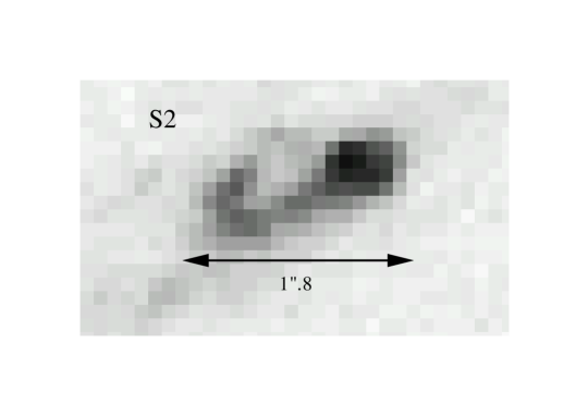
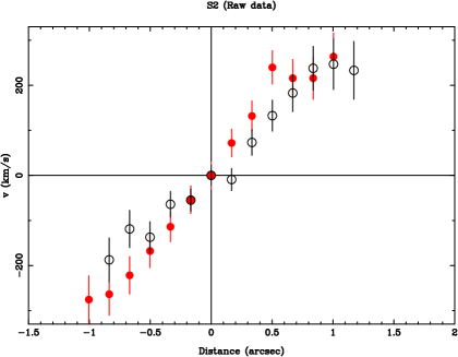
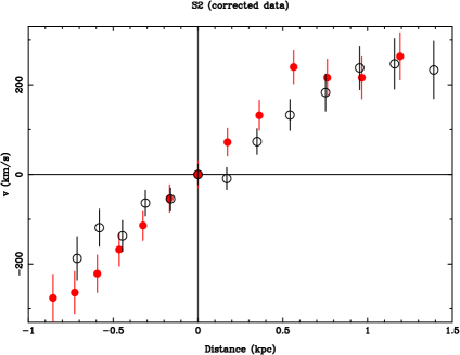
Figure 5: Spatially resolved emission lines in AC114-S2. Top panel: HST/WFPC2 ($R$-band/F702W) close image of the lensed galaxy AC114-S2. Mid panel: Raw velocity profiles (in km s^-1) versus angular distance (in arcsec), as measured on the 2D spectra from the central velocities of $\rm H{\alpha}$ (open dots) and [O iii] $\lambda$5007 (full dots) emission lines. Bottom panel: Lens corrected velocity profiles.

The virial mass derived for AC114-A2, and the largest determination for AC114-S2, a few $10^{10}M_{\sun}$, is of the same order as the typical values found for LBGs (e.g. Pettini et al. 2001). In contrast, AC114-S2 is about one magnitude brighter than AC114-A2, and one magnitude fainter than the typical LBGs in the rest-frame $B$-band. Thus, the $M/L_{\rm B}$ ratio of AC114-S2 in solar units ranges between 0.20 and 0.5, the lower value being quite similar to that of the LBGs at $z\sim 3$, whereas AC114-A2 has a $M/L_{\rm B}=2$, a ratio $\sim 20$ times higher than for LBGs. After dust extinction correction, we obtain $M/L_{\rm B}\sim$ 0.15 and 0.6 for AC114-S2 and AC114-A2 respectively, using the dynamical mass for S2. It is probable that both velocities and masses have been underestimated because of the limited sensitivity of the observations, since we see only the inner cores of the galaxies where star formation is the strongest.

6 Discussion

Table 5: Physical properties of high-redshift ($z\geq 2$) galaxies. Abundance ratios and SFRs are without extinction correction.

Galaxy	$z$	$M_{\rm B}$	12+log(O/H)	log(N/O)	${\rm SFR_{UV}}$	${\rm SFR_{H\alpha}}$	$M_{\rm vir}$ ($10^{10}$ M⊙)
AC 114-S2	1.867	$-$20.60	$7.25\pm 0.2$	$<-1.32$	4.4	30	$0.53\pm 0.12$
AC 114-A2	1.869	$-$19.80	$8.94\pm 0.2$	$-0.42\pm 0.2$	1.1	15	$2.36\pm 0.67$
CFg	2.313	$-$22.28	$7.8-8.7$	…	11	54	7.0
MS 1512-cB58	2.729	$-$22.04	$8.39\pm 0.2$	$-1.24\pm 0.2$	16	18	1.8
Lynx 2-9691	2.888	$-$23.19	$8.3-8.8$	…	11	80	5.2
Q0201+113 C6	3.055	$-$22.20	$7.6-8.8$	…	27	17	1.2
SSA22a D3	3.069	$-$22.59	$8.0-8.6$	…	38	24	…
Q1422+231 D81	3.104	$-$22.91	$7.7-8.7$	…	45	74	…
DSF 2237+116 C2	3.333	$-$23.97	$7.6-8.8$	…	44	75	5.5
B2 0902+342 C12	3.387	$-$22.84	$7.6-8.8$	…	42	61	…

Table 5 summarizes the physical properties for high-redshift ($z\ga 2$) galaxies. To date there is only one LBG in which chemical abundances have been determined with some degree of confidence, the gravitationally lensed galaxy MS 1512-cB58 at $z=2.729$ (Teplitz et al. 2000; Pettini et al. 2002a). Here we provide accurate chemical abundance measurements for the two high-redshift galaxies: AC114-S2 and AC114-A2.

In terms of SFRs without extinction correction, the two lensed low-luminosity galaxies A2 and S2 have ${\rm SFR_{1500}\ll SFR_{H\alpha}}$, while in LBGs at $z\sim 3$ ${\rm SFR_{1500}}\sim{\rm SFR_{H\alpha}}$ (within 15%). Note that a factor of two still remains between the two SFRs of S2 when using the latest calibrations by Rosa-Gonzalez et al. (2002). As shown in Section 5.1, a large E(B-V) value is needed to reconcile the UV/optical SFR values for these two objects. Unfortunately, we cannot derive an independent reddening estimate for S2 and A2, e.g. using the Balmer decrement $\rm H{\alpha}$/$\rm H{\beta}$..

6.1 The metallicity–luminosity relationship

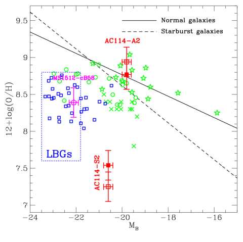
Figure 6: Oxygen abundance ($12+\log(\rm O/H)$) as a function of $B$-band absolute magnitude. The metallicity–luminosity relations for nearby “normal” (solid line; Kobulnicky & Zaritsky 1999) and starburst (dashed line; Mouhcine & Contini 2002; Melbourne & Salzer 2002) galaxies are shown. The location of the two $z\sim 1.9$ galaxies S2 and A2 in the lensing cluster AC 114 is shown without extinction correction (empty squares) and assuming a reddening E(B-V)=0.3 and 0.4 for S2 and A2 respectively (filled squares). We show for comparison samples of intermediate-redshift galaxies: UV-selected galaxies at $z\sim 0.1-0.4$ (circles; Contini et al. 2002), emission-line galaxies at $z\sim 0.1-0.5$ (stars; Kobulnicky & Zaritsky 1999), and at $z\sim 0.5-0.7$ (crosses; Hammer et al. 2001). The location of high-redshift ($z\sim 3$) Lyman break galaxies (LBGs) is shown as a blue box encompassing the range of O/H and $M_{\rm B}$ derived for these objects (Pettini et al. 2001). High-redshift ($1.4<z<3.4$) galaxies with oxygen abundances and $B$-band magnitudes derived from rest-frame UV spectra (Mehlert et al. 2002) are shown as blue squares.

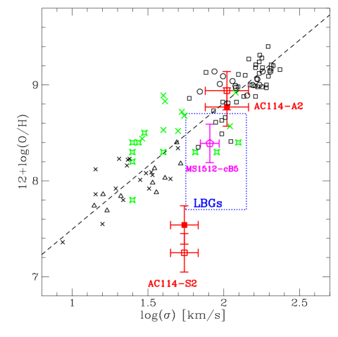
Figure 7: Oxygen abundance ($12+\log(\rm O/H)$) as a function of the line-of-sight velocity dispersion ($\sigma$). The location of AC114-S2 and AC114-A2 is shown without extinction correction (empty squares) and assuming a reddening E(B-V)=0.3 and 0.4 for S2 and A2 respectively (filled squares). We show for comparison samples of nearby galaxies: Hii galaxies (triangles; Telles & Terlevich 1997), dwarf galaxies (crosses; Richer & McCall 1995), late-type spirals (squares; Zaritsky, Kennicutt & Huchra 1994) and early-type spirals (circles; Oey & Kennicutt 1993). The dashed line is a linear fit to these samples. Intermediate-redshift galaxy samples are: emission-line galaxies at $z\sim 0.1-0.5$ (stars; Kobulnicky & Zaritsky 1999), and at $z\sim 0.5-0.7$ (crosses; Hammer et al. 2001). The location of high-redshift ($z\sim 3$) Lyman break galaxies (LBGs) is shown as a blue box encompassing the range of O/H and $\sigma$ derived for these objects (Pettini et al. 2001).

We can study the evolution with redshift of the fundamental scaling relation between galaxy luminosity and metallicity (Contini et al. 2002 and references therein). For nearby galaxies, this relation extends over $\sim 10$ magnitudes in luminosity and $\sim 2$ dex in metallicity.

The high-redshift sample is best compared to nearby galaxies where metallicities are derived using the same empirical strong line method. Figure 6 shows the relations for nearby i) “normal” irregular and spiral galaxies (solid line; Kobulnicky & Zaritsky 1999) and ii) starburst galaxies (dashed line; Mouhcine & Contini 2002; Melbourne & Salzer 2002), as well as the high-redshift sample from Table 5. Three samples of intermediate-redshift galaxies are also shown for comparison: UV-selected star-forming galaxies at $z\sim 0.1-0.4$, emission-line galaxies at $z\sim 0.1-0.5$ (Kobulnicky & Zaritsky 1999), and luminous compact emission-line galaxies at $z\sim 0.5-0.7$ (Hammer et al. 2001).

It is immediately obvious that high-redshift galaxies do not conform to today’s luminosity–metallicity relation for both “normal” and starburst galaxies. Even allowing for the uncertainties in the determination of O/H, high-redshift galaxies have much lower oxygen abundances than one would expect from their luminosities. This result, already revealed by previous studies (Kobulnicky & Koo 2000; Pettini et al. 2001; Contini et al. 2002), is secured with the addition of the low-luminosity and low-metallicity galaxy S2.

One interpretation of this result is that high-redshift galaxies are undergoing strong bursts of star formation which raise their luminosities above those of nearby galaxies with similar chemical composition. Another possibility is that the whole metallicity–luminosity relation is displaced to lower abundances at high redshifts, when the Universe was younger and the time available for the accumulation of the products of stellar nucleosynthesis was shorter. It should be possible to quantify this effect by measuring metallicities in samples of galaxies at different redshifts (e.g. Mehlert et al. 2002). As shown in Figure 6, intermediate-redshift galaxies seem to follow the luminosity–metallicity relation derived for nearby starburst galaxies (dashed line). Unfortunately, to date there is no sample of galaxies with known chemical abundances to fill the gap between $z\sim 0.5$ and $z\sim 2$.

The location of A2 is more surprising. It does not follow the trend of high-redshift objects. Instead, it lies on the luminosity–metallicity relation of nearby objects and has the highest metallicity of any high-redshift ($z\geq 2$) galaxy.

We compute the intrinsic $M_{\rm I}$ from the observed $K$-band magnitudes (2.2 $\mu$m corresponds to 7600 Å at $z\sim 1.9$) for S2 and A2. We found the same value $M_{\rm I}=-23.2$ for S2 and A2. This suggests that S2 and A2 may have the same stellar masses, since in the $I$ band we have access to the old stellar population which dominates the stellar mass. But the relatively high nitrogen abundance in AC114-A2 and MS 1512-cB58 suggests the presence of an older population of stars than in AC114-S2.

In Figure 7 we plot the oxygen abundance ($12+\log(\rm O/H)$) against the line-of-sight velocity dispersion ($\sigma$) for S2 and A2 and other relevant samples of nearby (Telles & Terlevich 1997; Richer & McCall 1995; Zaritsky, Kennicutt & Huchra 1994; Oey & Kennicutt 1993), intermediate (Kobulnicky & Zaritsky 1999; Hammer et al. 2001) and high redshift (see Table 5) galaxies. This diagram corresponds to a crude mass–metallicity sequence. The location of AC114-A2 is fully compatible with that of low-redshift galaxies. However, the oxygen abundance of AC114-S2 is much smaller than the corresponding value for low-$z$ galaxies of similar velocity dispersions. The situation is even more dramatic if we consider the velocity gradient derived under the disk-like rotation curve hypothesis (see sect. 5.3). Taken at face value, it would appear that the slope of the mass–metallicity relation for galaxies with $z\geq 2$ is different from that of low-$z$ galaxies.

6.2 The N/O versus O/H relationship

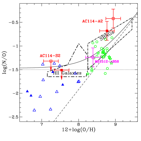
Figure 8: Nitrogen-to-oxygen (N/O) abundance ratio as a function of oxygen abundance ($12+\log(\rm O/H)$). The location of the two $z\sim 1.9$ galaxies S2 and A2 in the lensing cluster AC 114 is shown without extinction correction (empty squares) and assuming a reddening E(B-V)=0.3 and 0.4 for S2 and A2 respectively (filled squares). Two comparison samples of nearby star-forming galaxies are shown (see Contini et al. 2002 for references): starburst nucleus galaxies (dot – short dash line) and Hii galaxies (short dash – long dash line). We show, for comparison, samples of intermediate-redshift galaxies: UV-selected galaxies at $z\sim 0.1-0.4$ (circles; Contini et al. 2002), and emission-line galaxies at $z\sim 0.1-0.5$ (stars; Kobulnicky & Zaritsky 1999). The location of Damped Ly$\alpha$ systems (triangles, filled symbols are upper limits; Pettini et al. 2002b) is shown for comparison. Theoretical curves for a primary (dotted line), a secondary (dashed line), and a primary + secondary (solid line) production of nitrogen (Vila-Costas & Edmunds 1993) are shown.

In Figure 8, we examine the location of S2 and A2 in the N/O versus O/H relationship. The behavior of N/O with increasing metallicity offers clues about the history of chemical evolution of galaxies and the stellar populations responsible for producing oxygen and nitrogen. The location of the two $z\sim 1.9$ galaxies AC114-S2 and AC114-A2 are shown without extinction correction (empty squares) and assuming a reddening E(B-V)=0.3 and 0.4 for S2 and A2 respectively (filled squares). For comparison, we show in Figure 8 the location of nearby star-forming galaxies: starburst nucleus galaxies (SBNGs) and Hii galaxies (see Contini et al. 2002 for references). We also plot samples of intermediate-redshift galaxies: UV-selected galaxies at $z\sim 0.1-0.4$ (Contini et al. 2002), and emission-line galaxies at $z\sim 0.1-0.5$ (Kobulnicky & Zaritsky 1999). The location of Damped Ly$\alpha$ systems (Pettini et al. 2002b) is also shown.

The sample of high-redshift ($z\geq 2$) galaxies with measured N/O abundances is still very small: A2 and S2 from this paper, and MS 1512-cB58 at $z\sim 2.7$ (see Table 5). Surprisingly, these three galaxies have very different locations in the N/O vs. O/H diagram. S2 is a low-metallicity object ($12+\log(\rm O/H)$ $\sim 7.25$; Z $\sim 0.03$ Z_⊙) with a low N/O ratio (N/O $<-1.32$), similar to those derived in the most metal-poor nearby Hii galaxies. In contrast, A2 is a metal-rich galaxy ($12+\log(\rm O/H)$ $\sim 8.94$; Z $\sim 1.3$ Z_⊙) with a high N/O abundance ratio (N/O $\sim-0.42$), similar to those derived in the most metal-rich massive SBNGs. The position of MS 1512-cB58 is intermediate between these two extremes showing abundance ratios typical of low-mass SBNGs and intermediate-redshift galaxies (see Fig. 8).

A natural explanation for the variation of N/O at constant metallicity is the time delay between the release of oxygen and that of nitrogen into the ISM (e.g. Contini et al. 2002, and references therein), while maintaining a universal IMF and standard stellar nucleosynthesis. The “delayed-release” model assumes that star formation is an intermittent process in galaxies (e.g. Edmunds & Pagel 1978; Garnett 1990; Coziol et al. 1999) and predicts that the dispersion in N/O is due to the delayed release of nitrogen produced in low-mass longer-lived stars, compared to oxygen produced in massive, short-lived stars.

Following this hypothesis and new chemical evolution models (Mouhcine & Contini 2002), we might interpret the location of S2 and A2 in the N/O versus O/H diagram in terms of star formation history and evolutionary stage of these galaxies. The low O/H and N/O abundance ratios found in S2 might indicate a relatively young age for this object which experienced two or three bursts of star formation at most in the recent past. A2 seems on the contrary much more evolved. The location of this galaxy in the N/O versus O/H diagram indicates a relatively long star formation history with numerous powerful and extended starbursts.

7 Conclusions

We have presented in this paper the firsts results of our NIR spectroscopic survey of highly magnified high-redshift galaxies in the core of lensing clusters. Our first targets were AC114-S2 and AC114-A2, two lensed sources at $z\sim 1.9$. We have obtained, for the first time, the rest-frame optical emission lines of galaxies 1-2 magnitudes fainter than the LBGs studied in field surveys (e.g. Pettini et al. 1998, 2001; Kobulnicky & Koo 2000). The main results obtained in this paper are the following:

1. The SFRs derived from the $\rm H{\alpha}$ emission-line are systematically higher than the values deduced from the 1500Å  flux without dust extinction correction. The reddening values needed to obtain SFR_Hα/SFR_UV $\sim 1$ using the Calzetti et al. (2000) reddening law are E(B-V)=0.29 for AC114-S2 and E(B-V)=0.40 for AC114-A2, leading to corrected SFRs of 73 M_⊙ yr^-1 and 51 M_⊙ yr^-1 respectively. These results suggest that large dust extinction corrections are needed for intrinsically faint galaxies compared to field (brighter) LBG samples.

2. The large spectral coverage obtained, from [O ii] $\lambda\lambda$3726,3728 to $\rm H{\alpha}$+[N ii] $\lambda$6584, allows us to set strong constraints on the chemical abundance ratios (O/H and N/O) of these two faint galaxies. The behavior of S2 and A2 in terms of metallicity is different, and the two objects are also different from typical LBGs at $z\sim 3$, suggesting a different star formation history for galaxies of different luminosities.

3. The virial masses derived from the line-of-sight velocity dispersions are of the order of $5\times 10^{9}$ M_⊙ for AC114-S2 and $\sim 10^{10}$ M_⊙ for AC114-A2. The line profiles of AC114-S2 are spatially resolved, leading to a velocity gradient of $\pm 240$ km s^-1, which yields a dynamical mass of $1.3\pm 0.3\times 10^{10}$ M_⊙ within the inner 1 kpc radius, under the hypothesis of a rotation curve with disk-like geometry. Although the $M/L_{\rm B}$ ratio of AC114-S2 is quite similar, within a factor of 2, to the values found for field ($\sim$ 1 mag brighter) LBGs, the corresponding value for AC114-A2 is about one order of magnitude higher. After dust extinction correction, we obtain $M/L_{\rm B}\sim$ 0.15 and 0.6 for S2 and A2 respectively.

In terms of SFRs, mass-to-light and chemical abundance ratios, the behaviour of S2 and A2 is rather close to that described by Guzmán et al. (1997) for their sample of compact emission-line galaxies in the HDF at $0.7\la z\la 1.4$. S2 would correspond to a young star-forming Hii galaxy, whereas A2 is more likely an evolved starburst.

The results obtained on the physical properties of AC114-S2 and AC114-A2 suggest that high-$z$ objects of different luminosities could have quite different star formation histories. However, the number of well observed high redshift objects is currently very small and larger samples in both redshift (1.5 $\,\stackrel{{\scriptstyle<}}{{\scriptstyle\sim}}\,$ z $\,\stackrel{{\scriptstyle<}}{{\scriptstyle\sim}}\,$ 6) and luminosity are required. This could be achieved with the new generation of multi-object NIR spectrographs for the 10m class telescopes, such as KMOS on the VLT or EMIR on the GTC.

- (1) Altieri, B., Metcalfe, L., Kneib, J.-P., et al., 1999, A&A, 343, L65
- (2) Bézecourt, J., Soucail, G., Ellis, R. S., Kneib, J.-P., 1999, A&A, 351, 433
- (3) Calzetti, D., Armus, L., Bohlin, R. C., Kinney, A. L., Koornneef, J., Storchi-Bergmann, T., 2000, ApJ, 533, 682
- (4) Campusano, L.E., Pelló, R., Kneib, J.-P., et al., 2001, A&A, 378, 394
- (5) Contini, T., Treyer, M. A., Sullivan, M., Ellis, R. S., 2002, MNRAS, 330, 75
- (6) Coziol, R., Reyes, R. E. C., Considère, S., Davoust, E., Contini, T., 1999, A&A, 345, 733
- (7) Cuby, J.G., Lidman, C., Moutou, C., Johnson, R., Doublier, V., 2002, ISAAC User Manual, v1.10.1
- (8) Dopita, M. A., Evans, I. N., 1986, ApJ, 307, 431
- (9) Ebbels, T. M. D., Le Borgne, J.-F., Pelló, R., et al., 1996, MNRAS, 281, L75
- (10) Ebbels, T. M. D., Ellis, R. S., Kneib J. -P., et al., 1998, MNRAS, 295, 75
- (11) Edmunds, M. G., Pagel, B. E. J., 1978, MNRAS, 185, 77
- (12) Edmunds, M. G., Pagel, B. E. J., 1984, MNRAS, 211, 507
- (13) Ellis, R., Santos, M. R., Kneib, J., Kuijken, K., 2001, ApJ, 560, L119
- (14) Gallego, J., Zamorano, J., Aragón-Salamanca, A., Rego, M., 1995, ApJ, 455, L1
- (15) Garnett, D. R., 1990, ApJ, 363, 142
- (16) Guzmán, R., Gallego, J., Koo D. C., Phillips, A. C., Lowenthal J.D., Faber S. M., Illingworth G. D., Vogt N. P., 1997, ApJ, 489, 559
- (17) Hammer, F., Gruel, N., Thuan, T. X., Flores, H., Infante, L., 2001, ApJ, 550, 570
- (18) Heckman, T. M., Robert, C., Leitherer, C., Garnett, D. R., van der Rydt, F., 1998, ApJ, 503, 646
- (19) Hu, E. M., Cowie, L. L., McMahon, R. G., et al., 2002, ApJ, 568, L75
- (20) Ivison, R. J., Smail, I., Barger, A. J., et al., 2000, MNRAS, 315, 209
- (21) Kennicutt, R.C.,Jr., 1998, ARA&A, 36, 189
- (22) Kneib, J.-P., Ellis, R. S., Smail, I., Couch, W. J., Sharples, R. M., 1996, ApJ, 471, 643
- (23) Kobulnicky, H. A., Zaritsky, D., 1999, ApJ, 511, 118
- (24) Kobulnicky, H. A., Kennicutt, R. C., Pizagno, J. L., 1999, ApJ, 514, 544
- (25) Kobulnicky, H. A., Koo, D. C., 2000, ApJ, 545, 712
- (26) McCall, M. L., Rybski, P. M., Shields, G. A., 1985, ApJS, 57, 1
- (27) McGaugh, S. S., 1991, ApJ, 380, 140
- (28) Mehlert, D., Seitz, S., Saglia, R.P., et al., 2001, A&A, 379, 96
- (29) Mehlert, D., Noll, S., Appenzeller, I., et al. 2002, A&A, 393, 809
- (30) Melbourne, J., Salzer, J. J., 2002, AJ, 123, 2302
- (31) Mouhcine, M., Contini, T., 2002, A&A, 389, 106
- (32) Natarajan, P., Kneib, J.P., Smail, I., Ellis, R.S., 1998, ApJ, 499, 600
- (33) Oey, M. S., Kennicutt, R. C., 1993, ApJ, 411, 137
- (34) Osterbrock, D. E., 1989, Astrophysics of Gaseous Nebulae and Active Galactic Nuclei, University Science Books:Mill Valley CA
- (35) Pagel, B. E. J., Edmunds, M. G., Blackwell, D. E., Chun, M. S., Smith, G., 1979, MNRAS, 189, 95
- (36) Pagel, B. E. J., Edmunds, M. G., Smith, G., 1980, MNRAS, 193, 219
- (37) Pagel, B. E. J., Simonson, E. A., Terlevich, R. J., Edmunds, M. G., 1992, MNRAS, 255, 325
- (38) Pelló, R., Kneib, J.-P., Le Borgne J.-F., et al., 1999, A&A, 346, 359
- (39) Pettini, M., Kellogg, M., Steidel, C. C., Dickinson, M., Adelberger, K. L., Giavalisco, M., 1998, ApJ, 508, 539
- (40) Pettini, M., Steidel, C. C., Adelberger, K. L., Dickinson, M., Giavalisco, M., 2000, ApJ, 528, 96
- (41) Pettini, M., Shapley, A. E., Steidel, C. C., et al., 2001, ApJ, 554, 981
- (42) Pettini, M., Rix, S. A., Steidel, C. C., Adelberger, K. L., Hunt, M. P., Shapley, A. E., 2002a, ApJ, 569, 742
- (43) Pettini, M., Ellison, S. L., Bergeron, J., Petitjean, P., 2002b, A&A, 391, 21
- (44) Pilyugin, L. S., 2000, A&A, 362, 325
- (45) Pilyugin, L. S., 2001, A&A, 369, 594
- (46) Richer, M. G., McCall, M. L., 1995, ApJ, 445, 642
- (47) Rosa-Gonzalez, D., Terlevich, E., Terlevich, R, 2002, MNRAS, 332, 283
- (48) Rousselot, P., Lidman, C., Cuby, J.-G., Moreels, G., Monnet, G., 2000, A&A, 354, 1134
- (49) Shapley, A. E., Steidel, C. C., Adelberger, K. L., Dickinson, M., Giavalisco, M., Pettini, M., 2001, ApJ, 562, 95
- (50) Skillman, E. D., 1989, ApJ, 347, 883
- (51) Smail, I., Couch, W. J., Ellis, R. S., Sharples, R. M., 1995, ApJ, 440, 501
- (52) Smail, I., Dressler, A., Kneib, J., et al., 1996, ApJ, 469, 508
- (53) Smail, I., Ivison, R. J., Blain, A. W., 1997, ApJ, 490, L5
- (54) Smail, I., Ivison, R. J., Kneib, J.-P., et al., 1999, MNRAS, 308, 1061
- (55) Steidel, C. C., Giavalisco, M., Dickinson, M., Adelberger, K. L., 1996, AJ, 112, 352
- (56) Steidel, C. C., Adelberger, K. L., Giavalisco, M., Dickinson, M., Pettini, M., 1999, ApJ, 519, 1
- (57) Telles, E., Terlevich, R., 1997, MNRAS, 286, 183
- (58) Teplitz, H. I., Mc Lean, I. S., Becklin, E. E., et al., 2000, ApJ, 533, L65
- (59) Thurston, T. R., Edmunds, M. G., Henry, R. B. C., 1996, MNRAS, 283, 990
- (60) Vila Costas, M. B., Edmunds, M. G., 1993, MNRAS, 265, 199
- (61) Zaritsky, D., Kennicutt, R. C., Huchra, J. P., 1994, ApJ, 420, 87