Local Magnetohydrodynamical Models of Layered Accretion Disks

Abstract

Using numerical MHD simulations, we have studied the evolution of the magnetorotational instability in stratified accretion disks in which the ionization fraction (and therefore resistivity) varies substantially with height. This model is appropriate to dense, cold disks around protostars or dwarf nova systems which are ionized by external irradiation of cosmic rays or high-energy photons. We find the growth and saturation of the MRI occurs only in the upper layers of the disk where the magnetic Reynolds number exceeds a critical value; in the midplane the disk remains queiscent. The vertical Poynting flux into the “dead”, central zone is small, however velocity fluctuations in the dead zone driven by the turbulence in the active layers generate a significant Reynolds stress in the midplane. When normalized by the thermal pressure, the Reynolds stress in the midplane never drops below about 10% of the value of the Maxwell stress in the active layers, even though the Maxwell stress in the dead zone may be orders of magnitude smaller than this. Significant mass mixing occurs between the dead zone and active layers. Fluctuations in the magnetic energy in the active layers can drive vertical oscillations of the disk in models where the ratio of the column density in the dead zone to that in the active layers is $<10$. These results have important implications for the global evolution of a layered disk, in particular there may be residual mass inflow in the dead layer. We discuss the effects that dust in the disk may have on our results.

1 Introduction

One of the most promising mechanisms for angular momentum transport in accretion disks is magnetohydrodynamical (MHD) turbulence driven by the magnetorotational instability (MRI) (Balbus & Hawley 1998). For the instability to be present, the ionization fraction $x=n_{e}/n_{H}$ (where $n_{e}$ and $n_{H}$ are the number density of electrons and neutral hydrogen respectively) must be high enough that the neutral-ion collision frequency is greater than the local epicyclic frequency (Blaes & Balbus 1994). This condition can be met at very small values of $x$. For example, at $r=1$ AU in a disk with a density of $n=10^{13}$ cm^-3, linear instability requires $x>10^{-11}$. The fact that such low values of $x$ are sufficient to keep the gas and magnetic field well coupled implies that non-ideal MHD effects are important only in a few circumstances, such as in protostellar disks (see, e.g. Stone et al. 2001), or disks in dwarf novae systems (Gammie & Menou 1998).

The nonlinear evolution of the MRI in non-ideal MHD has been studied in several different regimes. If the ions and electrons are well coupled to the magnetic field, but the neutrals drift relative to the ionized species, the plasma is in the ambipolar diffusion regime. Hawley & Stone (1997) used two-fluid simulations to study the saturation of the MRI in this case. On the other hand, if collisions are so frequent that not only are the ions and neutrals well coupled, but also electrical currents are damped, then the plasma is in the Ohmic dissipation regime (Jin 1996; Sano & Miyama 1999). Saturation of the MRI in this case has been studied by Sano, Inutsuka, & Miyama (1998), and Fleming, Stone, & Hawley (2000, hereafter FSH), these authors find sustained MHD turbulence requires the magnetic Reynolds number $Re_{M}=C_{s}^{2}/\eta\Omega\gtrsim 10^{4}$ (where $C_{s}$ is the sound speed, $\Omega$ the rotatonal frequency, and $\eta$ the coefficent of resistivity) for poloidal fields with no net flux. Finally, if the positive and negative charge carriers can drift relative to one another, the plasma is in the Hall regime. The linear properties of the MRI are modified in unexpected ways in Hall MHD (Wardle 1999; Balbus & Turquem 2001); the nonlinear saturation of the MRI in Hall MHD has recently been studied by Sano & Stone (2002a; 2002b).

Previous studies of the saturation of the MRI in non-ideal MHD have all been designed to study the local physics of the instability, and have therefore used a local approximation termed the shearing box (Hawley, Gammie, & Balbus 1995, hereafter HGB) with homogeneous initial conditions. In this case, the computational domain represents a small region deep in the interior of the disk. However, there are a variety of important questions that can only be addressed by including the vertical structure of the disk. For example, for the case of ideal MHD, local simulations of vertically stratified disks have been used to study buoyancy of MRI amplified field (Brandenburg et al. 1995; Stone et al. 1996, hereafter SHGB) and the formation of strongly magnetized coronae above weakly magnetized disks (Miller & Stone 1999).

There are reasons to expect even more interesting vertical structure in weakly ionized disks. If the disk is too cold for thermal ionization of rare earth elements to be important ($T\lesssim 800$ K (Umebayashi 1983)), then the only sources of ionization will be nonthermal, for example irradiation of the disk by cosmic rays or high-energy photons. At the interstellar ionization rate due to cosmic rays, $\zeta\approx 10^{-17}~{}{\rm s}^{-1}$, the surface layers will be kept sufficiently ionized that they will be well coupled to the magnetic field (Gammie 1996). (The presence of small dust grains can significantly change this picture, however, and lead to much lower ionization fractions, Wardle & Ng 1999; Sano et al. 2000. This will be discussed further in §2.2.) However, the cosmic ray flux is attenuated towards the disk midplane, meaning the ionization fraction drops significantly, and non-ideal MHD effects become important. This has led Gammie (1996) to propose a “layered” model for weakly ionized disks, in which the surface layers are well coupled to the magnetic field and therefore turbulent (the “active layers”), while the midplane is decoupled and queiscent (the “dead zone”). More recently, Fromang et al. (2002) have explored in more detail the ionization structure of protostellar disks, they find the extent of the dead zone is extremely sensitive to the mass accretion rate, the critical magnetic Reynolds number below which the MRI is suppressed, and the abundance of metals in the disk.

There are a number of interesting implications to Gammie’s model. In particular, since the accreting layers of the disk have a fixed depth in surface density, the mass accretion rate increases with the radius of the disk. Thus, steady-state solutions are not possible for layered disks, leading Gammie to suggest that layered accretion could account for FU Orionis outbursts in T Tauri disks as accumulated mass in the dead zone is flushed out by, e.g. gravitational instabilities. This idea has been explored further by Armitage, Livio, & Pringle (2001) by solving the one-dimensional evolution equation for the disk surface density. In addition, the layered disk model has important implications for dust coagulation and planet formation in protoplanetary disks, as the dead zone may provide a sheltered environment for both processes.

In this paper, we present three-dimensional numerical MHD calculations designed to explore the local dynamics of layered disks; that is vertically stratified accretion disks in which the ionization fraction (and therefore resistivity) varies with vertical height. We find the formation of active layers and a dead zone occurs naturally in such a model, with the critical magnetic Reynolds number found by FSH providing a good prediction of the demarcation between areas of high and low angular momentum transport. We are also able to measure the rate of mixing between the turbulent layers and the midplane, and how much heating there is in the midplane due to diffusion of magnetic energy from the active layers. Perhaps our most important result is that we find significant angular momentum transport in the dead layer by non-axisymmetric density waves driven by turbulent motions in the active layers. As discussed in §5, these results have interesting implications for the structure and evolution of layered disks.

The paper is organized as follows. In §2 we describe our numerical methods, initial conditions, and the profile of the resistivity adopted here. In §3 we discuss the results of simulations with initially vertical fields with zero net flux. In §4 we discuss the results of initially azimuthal fields with zero-net flux. Our conclusions are given in §5.

2 Method

2.1 Equations and Initial Conditions

We adopt the shearing box approximation (HGB) to evolve a local patch of the disk in a Cartesian frame that is in corotation at a radius $R_{0}$ and angular frequency $\Omega$. In this frame, $x,y,$ and $z$ correspond to the radial, toroidal, and vertical directions, respectively. In these coordinates the equations of isothermal MHD may be written as

$${{\partial\rho}\over{\partial t}}+{\bf\nabla}\cdot(\rho{\bf v})=0$$ (1)

$${{\partial{\bf v}}\over{\partial t}}+{\bf v}\cdot\nabla{\bf v}=-{1\over\rho}\nabla\left(P+{B^{2}\over 8\pi}\right)+{{{\bf B}\cdot\nabla{\bf B}}\over 4\pi\rho}-2{\bf\Omega}\times{\bf v}+3\Omega^{2}x{\bf{\hat{x}}}-\Omega^{2}z{\bf{\hat{z}}}$$ (2)

$${\partial{\bf B}\over{\partial t}}={\bf\nabla}\times[({\bf v}\times{\bf B})-\eta(z){\bf J}],$$ (3)

$${P=c^{2}_{s}\rho}$$ (4)

where $c_{s}$ is the sound speed, ${\bf J}=(c/4\pi){\bf\nabla}\times{\bf B}$ is the current density, and $\eta(z)$ is the Ohmic resistivity (which is assumed to be a fixed function of vertical height), and the other symbols have their usual meaning. The method used to compute the vertical profile of the resistivity $\eta(z)$ described in the next section. The term $-\Omega^{2}z{\bf{\hat{z}}}$ in the momentum equation (eq. 2) is the vertical component of the gravitational field of the central object. As in SHGB, we use an isothermal equation of state (equation 4) to prevent an increase in the scale height of the disk due to heating associated with turbulence in the nonlinear regime of the MRI.

All of our simulations begin with the disk in a state of hydrostatic equilibrium. Thus, the density profile is Gaussian,

$$\rho=\rho_{0}e^{-z^{2}/H^{2}}$$ (5)

where $H^{2}=2c^{2}_{s}/\Omega^{2}$ is the scale height of the disk. In order to facilitate comparison with SHGB we adopt the same parameters and initial conditions as that work. Thus, we set $\Omega=10^{-3}$, $H=1$, and $\rho_{0}=1$, leading to $c_{s}=7.071\times 10^{-4}$ and $P_{0}=5.0\times 10^{-7}$.

Our computational domain spans $H/2\leq x\leq H/2$, $0\leq y\leq 2\pi H$, and $-2H\leq z\leq 2H$. Our standard numerical resolution is $60\times 128\times 256$ grid points (equivalent to the high resolution runs in SHGB), except that in order to better resolve the vertical structure of the disk, we have used twice the number of grid points in $z$.

We study two types of initial magnetic field configurations: either initially purely vertical or purely azimuthal fields. In both cases the field strength is proportional to $\sin 2\pi x$, so there is zero net magnetic flux through our computational domain. The magnetic field amplitude is parametrized by $\beta$, the ratio of thermal to magnetic pressure. At the midplane of the disk, $\beta(0)=P(0)8\pi/B^{2}$, all of the simulations presented here begin with $\beta(0)=400$. The exponential decrease in pressure and density reduces the plasma parameter $\beta$ as well. From a local analysis in ideal MHD, the critical wavelength of the MRI $\lambda_{c}=9.18\beta^{-1/2}$ (HGB), therefore we expect that the most unstable wavelengths will increase with height. For azimuthal fields, the field strength is given a gaussian profile in the vertical direction so that $\beta$ is initially uniform throughout the volume.

We employ periodic boundary conditions in the azimuthal ($y$) direction, and either periodic (for initially vertical field runs) or reflecting (for initially azimuthal field runs) boundary conditions in the vertical ($z$) direction. In the radial ($x$) direction, shearing-periodic boundary conditions are implemented on all runs (HGB). Outflow boundary conditions that allow mass, momentum, and energy to flow out of the computational volume would provide a more realistic model for accretion disks; however, utilizing outflow conditions along the $z$ direction is problematic. As described in SHGB, when strong ($\beta<1$) tangled magnetic fields are advected through free boundaries, field loops are broken. As the ends of the loop relax, a large Lorentz force will act on the fluid near the boundary. This disturbance is capable of affecting the entire disk. Because strong, highly tangled magnetic fields are characteristic of MHD turbulence, we cannot use outflow conditions to study the nonlinear evolution of the MRI unless the boundary is sufficiently removed from the disk midplane. For example, local isothermal simulations performed by Miller & Stone (2000) found that at five scale heights above the disk, a magnetically dominated coronal region which is stable to the MRI is formed, thus outflow conditions can be applied there. Since our simulations do not exceed two scale heights above the disk, we must adopt either periodic or reflective boundary conditions. SHGB found that the choice of vertical boundary conditions did not significantly alter the vertical structure of the disk.

The initial velocity field is a Keplerian shear flow represented by $v_{y}=-3\Omega x/2$. The MRI is seeded with small amplitude, spatially uncorrelated fluctuations in the velocity field distributed randomly throughout the simulation volume.

2.2 Vertical Profile of Resistivity

Our simulations are motivated primarily by the expected structure of disks around young stellar objects. We consider disk radii at which thermal ionization processes are ineffective. For protostellar disks, these regions lie at a radius $\mathrel{\vbox{\offinterlineskip\hbox{$>$} \kern 1.29167pt\hbox{$\sim$}}}0.1AU$ (Gammie 1996). We examine the case where the electron fraction is constant with time and cosmic rays are the only source of ionization, although similar results are expected if ionization occurs via X-rays instead (Igea & Glassgold 1999).

The resistivity is related to the electron fraction $x$ by

$$\eta=6.5\times 10^{3}x^{-1}{\rm cm}^{2}{\rm s}^{-1}$$ (6)

(Hayashi 1981), and assuming overall charge neutrality, the electron density is determined by

$${dn_{e}\over dt}=\zeta n_{H}-\beta x^{2}n^{2}_{H}=0,$$ (7)

which yields

$$x=\left({\zeta\over{\beta n_{H}}}\right)^{1/2}.$$ (8)

where $\beta$ is the recombination coefficient. A standard gas phase recombination rate due to dissociative recombination is $\beta\simeq 8.7\times 10^{-6}T^{-1/2}$ cm³ s^-1 (Glassgold, Lucas, & Omont 1986). At the surface of the disk we assume the ionization rate due to cosmic rays is the interstellar value, $\zeta_{0}\simeq 10^{-17}s^{-1}$ (Spitzer & Tomasko 1968). (We neglect the effect that magnetized outflows, if present, may have on the flux of cosmic rays that reach the disk surface.) However, the flux of cosmic rays is exponentially attenuated within the disk, with a decay length of $\Sigma_{CR}=100{\rm g~{}cm}^{-2}$. Thus, the ionization rate within the disk, $\zeta(z)$, is

$$\zeta(z)\simeq\zeta_{0}e^{-\Sigma(z)/\Sigma_{CR}},$$ (9)

where the column density $\Sigma(z)=\int^{\infty}_{z}\rho dz^{\prime}$. Combining equations (6), (8), and (9) and normalizing with respect to disk scale height yields

$$\eta(z)=\eta_{0}\ {\rm exp}(-z^{2}/2){\rm exp}\left({{\Sigma_{0}\over\Sigma_{CR}}{1\over{2\sqrt{pi}}}\int^{\infty}_{z}e^{-z^{\prime 2}}dz^{\prime}}\right)$$ (10)

for an isothermal disk, where $\Sigma_{0}$ is the total column density through the disk.

Our expression for the resistive profile (equation 10) has two free parameters $\eta_{0}$ (the resistivity at the midplane) and the ratio $\Sigma_{0}/\Sigma_{CR}$. We choose the former so that the magnetic Reynolds number near the midplane $Re_{M}\lesssim 10^{3}$, this is below the critical value found by FSH for sustained turbulence and ensures the MRI will be damped in the midplane. The latter we choose to give a large dynamic range in the resitivity. Setting $\Sigma_{0}/\Sigma_{CR}\sim 30$ yields an $Re_{M}$ that varies by four orders of magnitude over two scale heights. Note this implies the disk surface density is 3000 gm cm^-3, about a factor of two larger than the value for the minimum solar nebula. The range of values chosen for $Re_{M}$ was limited by the Courant condition for numerical stability. Choosing values lower than $Re_{M}=100$ would have placed a substantial computational burden upon our simulation. Thus it is worth noting that our midplane values for $Re_{M}$ are somewhat higher than those expected in protostellar disks at radii near 1AU. For example, with a number density of $10^{13}cm^{-3}$, T=100 K, and a cosmic ray ionization rate $\zeta=10^{-17}s^{-1}$, the fractional ionization is $x=10^{-12}$. This yields a $Re_{M}\approx 1$. However, as our simulations will demonstrate, the values of $Re_{M}$ considered in this work are sufficient to stabilize the disk. Moreover, once the critical magnetic Reynolds number which stabilizes the disk is reached, we do not expect the dynamics (such as the Reynolds stress) in the dead zone to be significantly different at lower $Re_{M}$. However, we might expect that decreasing the value of $Re_{M}$ at the midplane for our simulations would result in an increase in the size of the dead zone and therefore a thinner active layer.

We have neglected effects of dust grains in this analysis. For a given ionization rate, the presence of small dust grains can greatly decrease the ionization fraction since the surface of grains can act as a catalyst for recombination reactions. If dust grains with an interstellar size distribution are mixed throughout the disk, it is unlikely that even the surface layers of the disk will be sufficiently ionized to be unstable to the MRI (Sano et al. 2000). However, dust grains may grow in size through coagulation, thereby decreasing their surface area and reducing their effect on the recombination rate. Alternatively, in the abscence of turbulence which keeps the grains well mixed vertically, they may sediment toward the midplane leaving the upper layers of the disk dust free. By neglecting the effects of grains, we restrict the applicability of our results to protostellar disks which are in the late stages of evolution, where grains have either settled to the midplane or grown too large to affect the recombination rate. The calculation of the self-consistent vertical structure of the disk in the presence of small grains requires following both the non-ideal MHD of the gas, as well as the dynamics of the grains driven by aerodynamic forces (to account for gravitational settling and turbulent mixing); such a calculation is beyond the scope of the current paper.

3 Vertical Fields with Zero-Net Flux

Table 1 summarizes the parameters and results of our numerical simulations. We first discuss the results from vertical field simulations, which are labeled by the prefix Z (toroidal field simulations, which are discussed in the next section, are labelled with the prefix Y). At the numerical resolution used here the ratio of the critical wavelength $\lambda_{c}$ of the MRI at the midplane (assuming ideal MHD) to the grid spacing $\Delta z$ ($\Delta y$) for poloidal (toroidal) fields is 30, indicating it should be captured if present. (With a finite resistivity, the critical wavelength increases, thus our estimate is a lower bound on the number of grid points per unstable wavelength.) Columns (4), (5), and (6) give the time- and volume-averaged values of magnetic field energy, Maxwell stress, and Reynolds stress in both the active layers and the dead zone, all normalized with respect to the midplane pressure. These averages are taken from late times, when the active layer has reached saturation. The location of the boundaries between the active layers and dead zone is measured from the calculations themselves; as discussed below the boundaries are generally located where $Re_{M}$ is equal to the critical value found by FSH.

3.1 A Model with a small dead zone

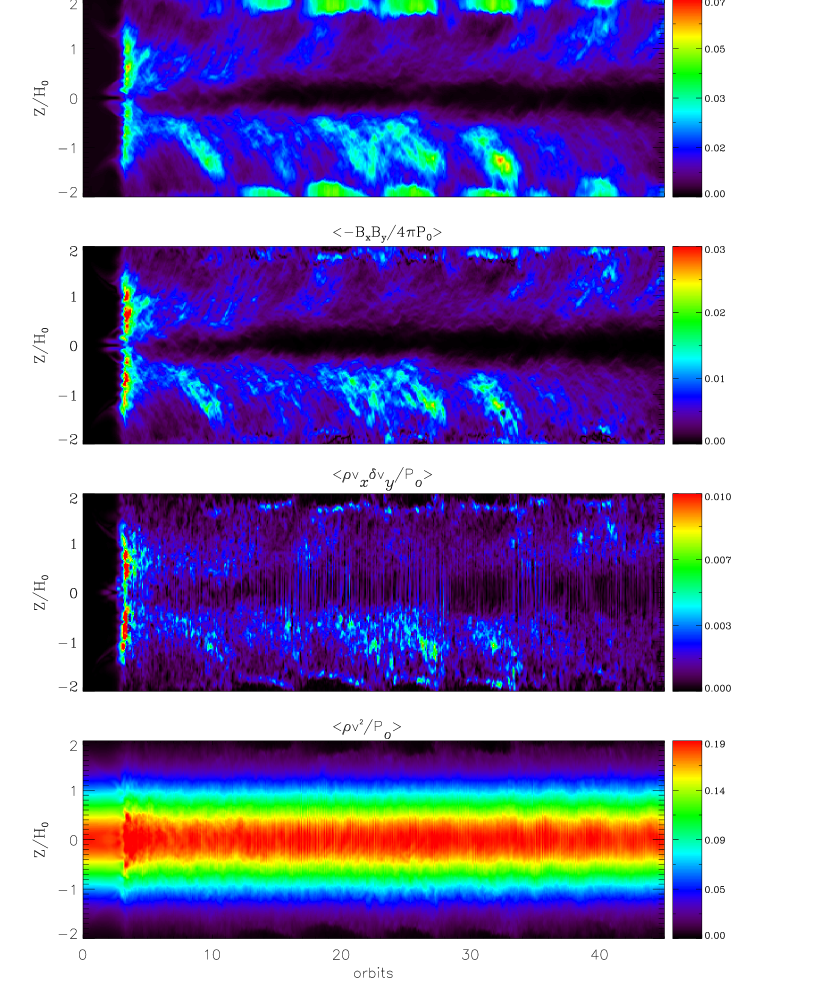
Figure 1: Spacetime plots of the horizontally averaged magnetic energy, Maxwell stress, Reynolds stress, and kinetic energy for the zero-net mean field run Z1. The dead zone is evident by orbit 5: turbulence has ceased within $|z/H|<0.4$, however the Reynolds stress is still non-zero in this region.

We first discuss run Z1, comparing it to the equivalent ideal MHD run Z4 (run Z4 is identical to run IZ2 in SHGB but with a higher resolution). The magnetic Reynolds number in Z1 varies from $1000$ at the midplane to $5.6\times 10^{6}$ at $z/H=2$. Figure 1 is a “spacetime” plot of horizontally averaged quantities $F(z,t)$ versus vertical height and time. The plot is created by horizontally averaging each four-dimensional quantity $f(x,y,z,t)$ via

$$F(z,t)={{\int\int f(x,y,z,t)dxdy}\over{\int\int dxdy}}.$$ (11)

The figure can be compared directly to figure 3 in SHGB.

The linear phase of the MRI occurs over the first three orbits of evolution. Suprisingly, the plot of magnetic energy shows the earliest growth occurs near the midplane, where the resistivity is highest and the growth rates of the MRI should be lowest. In fact, this growth is not associated with the MRI at all, but occurs as a consequence of reconnection in the initial field topology. In the highly resistive midplane, the oppositely directed vertical field components in the initial conditions reconnect, forming radial fields that are subsequently sheared by the differential rotation of the disk. This shear produces an azimuthal magnetic field which grows linearly with time. It is this azimuthal field that produces an increase in the magnetic energy. This process does not occur in ideal MHD runs.

The shear amplified field is soon overwhelmed by the exponentially growing MRI. The initial saturation of the MRI occurs around orbit 3; it is evident as a strong peak in the magnetic energy and other variables at this time. The highest field energy occurs at $|z/H|<1.5$ as a consequence of disk stratification. The decrease in density with increasing $|z|$ means that the Alfvén speed, and also critical wavelength $\lambda_{c}$, rise with increasing $|z|$. The increase in $\lambda_{c}$ lowers the peak magnetic field strength at saturation. In fact, some of the long wavelength modes near the top and bottom of the disk may exceed the length of our simulation volume and thus will not be present. Near $z=0$ (minimum $Re_{M}$), the field energy is reduced, indicating the shorter wavelength modes of the MRI have been damped by resistivity; only long wavelength modes develop in the midplane region. Note the maximum magnetic energy at orbit 3 has discrete peaks at various vertical positions. These are associated with the channel solution that occurs for vertical fields (Hawley & Balbus 1991; SHGB).

Beyond the linear phase (after orbit 3) we see the breakdown of the channel solution via parasitic instabilities (Goodman & Xu 1994) into MHD turbulence. In an ideal MHD run (cf. figure 3 of SHGB), this turbulence fills the entire volume of the disk. However, the variation of the resistivity with height causes a non-uniform structure in the disk: MHD turbulence is confined to the outer layers alone. Thus, as anticipated by Gammie (1996), the disk may be divided into two regions: two active layers near the surfaces of the disk (characterized by low resistivity and MHD turbulence), and a dead zone near the midplane (characterized by high resistivity and a quiescent flow). The dead zone forms spontaneasouly after saturation, by orbit 15 it is well developed. The boundary between zones is located at approximately $|z|=z_{B}=0.4$. At $|z|=z_{B}$ the magnetic Reynolds number $Re_{M}\sim 2\times 10^{4}$. This is in good agreement with the critical $Re_{M}$ obtained by FSH for zero mean poloidal fields in uniform disks. This dead zone persists throughout the remainder of the simulation. Given the location of the boundaries, and since the vertical profile of density is little changed from the initial state (eq. 5) (see below), the column density in the active layers $\Sigma_{a}$ compared to the dead zone $\Sigma_{d}$ follows directly from

$$\frac{\Sigma_{a}}{\Sigma_{d}}=\frac{2\int_{z_{B}}^{\infty}\exp(-z/H)^{2}}{\int_{-z_{B}}^{z_{B}}\exp(-z/H)^{2}}\approx 0.75$$ (12)

The two layer structure in the disk is evident in the plots of the Maxwell and Reynolds stress. Angular momentum transport via magnetic fields is confined to the active zone. Interestingly, although the Reynolds stress is reduced in the dead zone, it is not eliminated there. Figure 1 shows that there are irregular increases in Reynolds stress within the dead zone. Vertical striations in the plot of the Reynolds stress are associated with spiral density waves in the disk (SHGB). A comparison with the field energy reveals that the fluctuations in the Reynolds stress correspond with significant field energy increases in the active layers. Strong Lorentz forces in the active zone may be driving these fluctations well into the midplane region. We will examine this question in greater detail below.

The time-averaged vertical structure of the disk is shown in Figure 2, which plots the density, plasma $\beta$ parameter, magnetic and kinetic energy, and Maxwell and Reynolds stress averaged over orbits 15-45. The density retains its initial gaussian profile with the same scale height throughout the nonlinear evolution of the MRI, indicating thermal pressure is still the dominant force which balances gravity. Within the dead zone the effects of magnetic diffusion are clearly evident. At the midplane MHD turbulence has been suppressed resulting in an extremely weak ($\beta=1000$) field there. This is a significant decline in the field energy as compared to the outer regions; $\beta$ in the midplane is $\sim$ 100 times greater than in the active layers of the disk. The maximum value of $\beta$ in the dead zone is $\sim$ 22 times greater than the peak value in the ideal run Z4. However, in the dead zone of run Z1, the field rises by an order of magnitude as the demarcation line, $z=z_{B}$, is approached. By $z=1.0$, $\beta$ has declined to a value comparable to that at the corresponding point of the ideal run Z4. This steep increase in field energy is consistent with the high gradient in resistivity present in the dead zone.

Tables 1 and 2 list volume averaged values for a number of quantities in run Z1 in both the active layers and the dead zone. From the tables it is evident that the average magnetic energy is three times larger in the active layer than in the dead zone. The magnetic energy in the active layer is confined mostly to the azimuthal component, with $B^{2}_{y}\sim 7.5B^{2}_{x}\sim 17.5B^{2}_{z}$. Similar results are obtained in the ideal run BZ4 and in SGHB. Azimuthal field also dominates all other components in the dead zone as well. In all cases the background shear favors the growth of the azimuthal component. The amplitude of each of the field components in the active layers of run Z1 is significantly lower (by a factor of at least two) than in the corresponding locations in the ideal MHD runs. This is mostly due to the finite resistivity in the active layers themselves, rather than due to diffusion into the dead zone. This is shown by the magnitude of the Poynting flux

$$F_{P}={\int_{s}{\eta({\bf J\times B})\cdot{\bf dA}}}+{\int_{s}{B^{2}\thinspace{\bf v}\cdot{\bf dA}}}-{\int_{s}{({\bf v}\cdot{\bf B}){\bf B}\cdot{\bf dA}}}$$ (13)

measured at the boundaries between the active layers and dead zone in run Z1. The average magnetic energy flux out of the active regions in one orbit is only $0.3\%$ of the total magnetic energy in those regions. We conclude the lower field energy in those regions is a result of Ohmic dissipation within the active zone itself.

From Table 1, in the active regions the time- and volume-averaged Maxwell stress exceeds the Reynolds stress by a factor of $\sim 4$; consistent with the ideal MHD results (run Z4 and SHGB). However, as with field energy saturation amplitudes, the stress amplitudes in the active regions are reduced by about 50% compared to their values in the same volume of an ideal MHD simulation due to the finite resistivity in these layers. Within the dead zone, the Maxwell stress drops rapidly (see Figure 2). The time- and volume-averaged Maxwell stress in the dead zone is about 1/4 the value in the active layers. Interestingly, the same effect is not observed with the Reynolds stress. The average Reynolds stress in the dead zone is $\sim 60\%$ of the average Reynolds stress in the active layers, and $34\%$ of the average Reynolds stress for the ideal run. Since the drop in Reynolds stress in the dead zone is not as significant as the drop in Maxwell stress, the Reynolds stress is now the dominant mechanism by which transport may occur. Similar dominance of Reynolds stress over the Maxwell stress at low $Re_{M}$ was observed in the simulations performed by FSH.

When scaled by the thermal pressure at the midplane, the total stress in the active layers in run Z1 is $\alpha=W_{xy}/P_{0}=0.006$, whereas in the region within $|z|<0.4$, $\alpha=0.002$ The amplitude of the total stress at the midplane (which is dominated by the Reynolds stress) is much larger than expected from the uniform resistivity runs of FSH. For example, the minimum Reynolds stress (at the midplane) is about 50 times larger than the Reynolds stress for a uniform resitivity run with the same $Re_{M}$ from FSH. To test whether turbulence in the active layers is driving velocity fluctuations in the dead zone and producing an enhanced Reynolds stress there, we have measured the flux of kinetic energy,

$$F_{K}=\int_{S}(\rho v^{2}){\bf v}\cdot{\bf dA},$$ (14)

across the surfaces $|z|=0.5$. We find a net flux into the dead zone which transports $5\%$ of the average total kinetic energy into the active layers in one orbit. This greatly exceeds the magnitude of the Poynting flux into the dead zone.

Overshooting of turbulent eddies results in significant mas mixing between the active and the dead layers of the disk. The average mixing time (defined as the amount of time taken to transport the entire mass of the dead zone across the active zone boundary) was 3.8 orbits for this simulation. We find later that this time increases as the size of the active layer is decreased.

3.2 A Model with a Larger Dead Zone

Run Z2 is identical to Z1 except the resistivity at the midplane is increased so that $Re_{M}=100$ at $z=0$ and increases to $\sim 5.6\times 10^{5}$ at $|z|=2$. This simulation ran for 60 orbits. The qualitative evolution of this model is identical to run Z1: a queiscent region is formed by 15 orbits at the midplane of the disk which is surrounded by active, turbulent layers. Once again the boundary between the active and dead layers is the value of $z$ where $Re_{M}\sim 2\times 10^{4}$, in this model this occurs within $|z|<0.9$. Thus, the column density of the active layers compared to the dead zone is $\Sigma_{a}/\Sigma_{d}\approx 0.25$, three times smaller than in run Z1.

The time-averaged vertical structure of the disk in run Z2 is shown in Figure 3. Here all quantities have been averaged from orbit 30 to 60, after saturation has been reached in the active layers. As with the other simulations, the gaussian density profile remains constant. The lower $Re_{M}$ in the dead zone has had a significant effect on the field energy there; the maximum value of $\beta$ has grown by a factor of 8 over the peak for Z1. The total range in $\beta$ from the dead zone to the active layers is now over 5 orders of magnitude. From the plot of field energy the saturation amplitude in the active layers has been reduced to $20\%$ of its value in Z1 due to the higher resistivity. Within the active layers, the azimuthal component of magnetic field energy dominates by an even greater amount than in Z1; ordering is $B^{2}_{y}\sim 10B^{2}_{x}\sim 27.5B^{2}_{z}$, averaging from orbit 30 to 60. This is consistent with FSH, where it was found that increasing resistivity resulted in greater dominance of the azimuthal field. In figure 3 we see that the field energy drops off by 2 orders of magnitude between the active zone and the center of the dead zone. This is an order of magnitude greater than the drop off observed for Z1. The saturation amplitude of the kinetic energy are lower in all regions of the disk for Z2 as compared to Z1.

An interesting feature of the evolution of run Z2 is the excitation of vertical oscillations in the disk produced by asymmetrical magnetic pressures in the active layers. The two active layers act as independent dynamos, with local amplification of magnetic field balanced by resistive dissipation. There are significant temporal fluctuations in the total magnetic energy in the active layers associated with the turbulence. Since the two active layers are decoupled, these fluctuations are not correlated, leading to small differences in the magnetic pressure gradients at the boundary of the dead zone. These gradients excite vertical oscillations of the disk midplane with an amplitude of $0.1H$ and a period of 4 orbits. The oscillations begin around orbit 10 and continue for the remainder of the calculation with no significant change in amplitude. They do not appear to affect the internal dynamics of the active and dead zones, but might have interesting implications for the production of winds and outflows from the disk.

The time- and volume-averaged Maxwell stress in the active layers dominates over the Reynolds stress by $\sim 3.5$. When scaled by the thermal pressure, this leads to a total stress of $\alpha=W_{r\phi}/P_{0}=0.00126$ in the active regions, and $\alpha=0.00026$ in the dead zone ($|z|<0.9$). These represent reductions of $79\%$ and $91\%$ as compared to the active and dead zones of Z1. The higher average resistivity in these active layers as compared to Z1 reduces the saturated stress amplitudes. For example, the Maxwell stress in the active regions is $\sim 18\%$ of the value obtained in the active layers of Z1, and from $z=1$ to $z=0$ the Maxwell stress drops by approximately 4 orders of magnitude. This represents a far greater drop than occurred in the lower resitive run. However, much like Z1, the Reynolds stress does not suffer a similar decline in the midplane. From Figure 3, we see that the average Reynolds stress within the dead zone does not vary substantialy from its value in the active layer. As with Z1, the velocity fluctuations which give rise to the Reynolds stress are supported by transport of kinetic energy into this region from the active layers. The flux of kinetic energy into the dead zone during one orbit is $12\%$ of the average kinetic energy within the active layers. This transport ratio is larger than that which was obtained for Z1, due to the depressed saturation amplitudes in Z2. On the other hand, the average Poynting flux across the interface between the active and dead layers ($|z|=0.9$) is insignificant, with the net average value being only $\sim 0.15\%$ of the average total magnetic energy in the active regions.

The very small amplitude of the Reynolds stress might be a result of purely numerical effects rather than being driven by turbulence in the active layers. To test this, we have restarted run Z2 at orbit 45 with the Lorentz forces removed from the equations of motion (i.e. a pure hydrodynamics simulation). This restart ran for 10 orbits. The effect is immediate. Turbulent flow in the active layers, and the Reynolds stress it produces in the dead zone, quickly decays away on a timescale of only a few orbits. This result is in agreement with the Lorentz force off run performed by HGB. By orbit 55 (ten orbits after the restart), the Reynolds stress in the dead zone is 10 times smaller than when Z2 is continued with MHD. Thus we conclude that the Reynolds stress in the dead layer requires MHD turbulence in the active regions.

Another way to quantify the effect of increasing resistivity on the dynamics of an accretion disk is to measure the mixing time across an arbitrary boundary within the disk, defined as the time required for an amount of mass equal to the total mass within a volume to flow into that volume. The mass flux into the volume $|z|<0.5$ was measured for runs Z1, Z2, and Z4. (Note that these fluxes are measured at the same location, although the boundary of the dead zone and active layers is different in each case.) Consistent with our measurements of kinetic energy above, we find that increasing the resistivity decreases the mass flux into the volume $|z|<0.5$. The average mixing time measured for the ideal run, Z4, was 3.8 orbits. For the resistive run Z1, this time increases to 5.8 orbits, and for the highly resitive run Z2, it is 6.2 orbits. These results suggest that there is a decreasing level of interaction between the dead and active layers as resistivity is increased. Note that even though we have measured the mass flux at a location well within the dead zone of run Z2, the mixing time is still relatively short.

Finally, we have also run a model identical to runs Z1 and Z2, but with a very large resistivity at the midplane so that $Re_{M}=10$ there; this run is labelled Z3 in Table 1. In this case the magnetic Reynolds is so small throughout the entire volume of the disk that MHD turbulence cannot be sustained. There is transitory growth of the MRI in the early stages of evolution, however once the MRI saturates the field dies away and the disk becomes quiescent. For this reason the model was only run to 20 orbits; the time-averaged values of the Maxwell and Reynolds stress during this peroid are given in Table 1. In comparison to runs Z1 and Z2, the saturation amplitude of both quantities at this $Re_{M}$ is very small. Based on the results of FSH, sustained turbulence and transport can only be supported at such low values of $Re_{M}$ if the magnetic field has a net poloidal flux; our results are consistent with this finding.

4 Azimuthal Fields with Zero-Net Flux

To examine whether the saturated state of the MRI in a vertically stratified disk depends on the initial field geometry, we have run two simulations with a purely toroidal field, labeled Y1 and Y2 in Table 1. In run Y1, the profile of the resistivity was identical to that used in run Z1, that is $Re_{M}=1000$ at the midplane, to $Re_{M}=5.6\times 10^{6}$ at $|z|=2$. The resistivity was reduced in run Y2, so that $Re_{M}=5700$, at the midplane, to $Re_{M}=2.8\times 10^{7}$ at $|z|=2$. These simulations were performed at our standard resolution of $60\times 128\times 256$, and used reflective boundary conditions at the surfaces $z=-2$ and $z=2$.

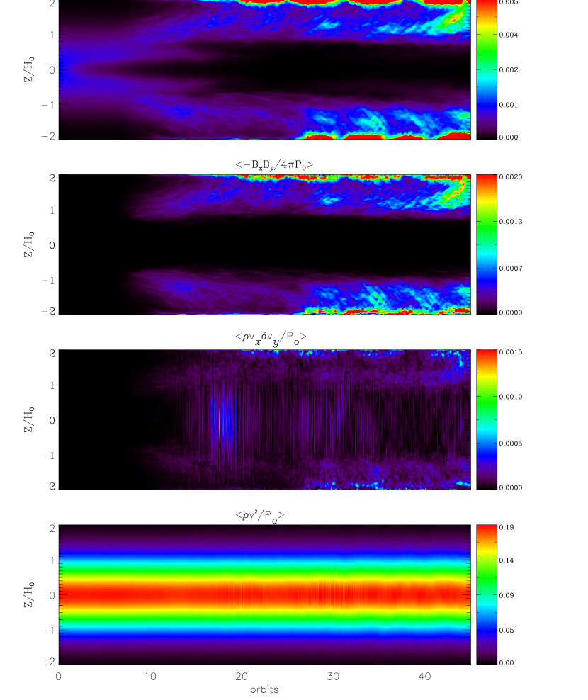
Figure 4: Spacetime plots of the horizontally averaged magnetic energy, Maxwell stress, Reynolds stress, and kinetic energy for the zero-net mean field run Y1

Figure 4 is a spacetime plot of the horizontally averaged magnetic energy, Maxwell stress, Reynolds stress, and kinetic energy for run Y1. As expected, the linear growth rate of the MRI on purely azimuthal fields is lower than for vertical fields (Balbus & Hawley 1992), thus saturation does not occur until orbit 20. Also note that shear amplification of radial fields generated by reconnection which is visible at early time in run Z1 (see Figure 1) does not occur here.

Beyond orbit 15, a dead zone ranging from $z=-1$ to $z=1$ is clearly evident within the disk. Despite the same profile of resistivity, this is approximately twice as large as the dead zone observed in Z1. The boundary for the dead zone occurs at $Re_{M}\sim 3\times 10^{5}$. This is an order of magnitude larger than the value of $Re_{M}$ that marks the boundary for the dead zone in BZ1. A similar change in critical $Re_{M}$ with initial field geometery was observed in FSH; an order of magnitude increase in the critical magnetic Reynolds number for instability for a uniform azimuthal compared to a uniform poloidal field geometry. The column density in the active layers compared to the dead zone is $\Sigma_{a}/\Sigma_{d}\approx 0.187$, five times smaller than in run Z1.

The volume-averaged properties of Y1 are more similar to run Z2 (which has roughly the same ration of column density in the dead zone to active layers) than run Z1, which has the same resistivity profile. This is because azimuthal fields are more strongly affected by magnetic diffusion than poloidal fields. For example, the magnetic energy in the active zone is approximately 10 times greater than in the dead zone. The ordering of field energy components in the active zone of Y1 is $B^{2}_{y}\sim 10B^{2}_{x}\sim 33B^{2}_{z}$, which is also similar to that in the corresponding region of Z2.

Figure 5 plots the vertical profiles of the density, plasma parameter $\beta$, magnetic and kinetic energy densities, and Maxwell and Reynolds stress averaged from orbits 30 to 45 for Y1. Note this is deep in the nonlinear regime, well after saturation of the MRI. We see that the saturation amplitude of field energy in the active zone is $2\times 10^{-3}$ (normalized by $P_{0}$) for Y1, which is $13\%$ of its value for Z1. Additionaly, the Maxwell stress in the active layers of Y1 is also only $13\%$ of its value for Z1, leading to $\alpha\sim 8\times 10^{-4}$ in the active layers. In the center of the dead zone ($|z|<0.5$), $\alpha\sim 5.7\times 10^{-5}$, a value two orders of magnitude lower than found for Z1. Finally, we find that the kinetic energy in the active region is also reduced by about an order of magnitude as compared to Z1, due to the decreased levels of MHD turbulence in the active layers.

The qualitative behavior of the Maxwell and Reynolds stress in these azimuthal runs is the same as in the poloidal runs; while the Maxwell stress suffers a substantial decline in the dead zone, the Reynolds stress is only slightly lower there than in the active region. In the active layers, Maxwell dominates over Reynolds stress by a factor of $\sim$ 4. This is the same ratio as in the poloidal field runs. However, within the dead zone, the steep decline of the Maxwell stress causes it to fall below the Reynolds stress. The closer we get to the midplane, the greater the Reynolds stress dominates. For example, within the volume enclosed by $|z|<0.5$, the average Reynolds stress is 4.7 times larger than the Maxwell stress. For the volume bounded by $|z|<0.2$, the Reynolds stress is two orders of magnitude greater than that observed in Z1 for $|z|<0.2$.

Run Y2 has a much lower resistivity in the midplane than Y1 discussed above, so that $Re_{M}=5700$ there. The properties of this run are given in Table 1. We find the production of only a tenous dead zone in the early stages of the evolution, which disappears once the active layers are fully saturated. Shortly after the onset of the MRI, we find that within the region $|z|<0.5$, average Maxwell stress is $\sim 10\%$ of its value in the outer regions. However, as the simulation progresses, the difference between the Maxwell stress in the inner and outer regions decreases. By orbit 40, the average Maxwell stress within $|z|<0.5$ has climbed to $\sim 60\%$ of its value in the outer regions. In addition, we find that at later stages in the simulation the Maxwell stress never falls below the Reynolds stress, even at the midplane. Correspondingly we find that angular momentum transport rates are high in the central regions of the disk during the last 20 orbits of the simulation. Clearly, the existence of a dead zone depends critically on whether or not the magnetic Reynolds number in the disk midplane is small.

5 Summary

Using numerical MHD simulations, we have studied the evolution of the MRI in stratified accretion disks including resitivity that varies with vertical height. The vertical profile of resistivity is computed assuming that the dominant source of ionization is external irradiation by cosmic rays (or perhaps X-rays), so that the ionization fraction drops dramatically below a penetration depth of $\Sigma_{CR}=100$ g cm^-2. This profile is appropriate for cold disks around young stellar objects, or in dwarf nova systems.

The evolution of two different initial field geometries were examined: a zero net mean poloidal field and a zero net mean azimuthal field. Additionaly, several different column densities for the disk were studied (models with larger column densities have a much higher resistivity at the midplane). In each case, we find the development of MHD turbulence is the less-resistive surface layers of the disk with a queiscent zone in the highly resistive midplane, consistent with the model of layered accretion put forward by Gammie (1996). The boundary between the active layers and the dead zone occurs at the location where the magnetic Reynolds number $Re_{M}$ is equal to the critical value found by FSH for MHD turbulence in the nonlinear regime of the MRI. For initially poloidal fields with zero net flux this critical value is of order $10^{4}$, for initially toroidal fields it is ten times larger. This criterion is therefore a useful means by which the scale of the dead zone may be determined in stratified disks. Since the critical value is smaller for fields with net flux, the size of the dead zone may be correspondingly smaller for that field geometry.

The active regions are charcterized by MHD turbulence and outward angular momentum transport. In these regions, as with ideal simulations, Maxwell stress is the significant source of angular momentum transport, dominating Reynolds stress by a factor of $\sim 4$. However, the saturation levels for field energy and Maxwell stress are less than those obtained in ideal MHD models since Ohmic dissipation in the active zone is never completely negligable.

Our simulations reveal some unexpected properties of the layered accretion disk model. For example, although the MRI is suppressed in the dead zone the Reynolds stress fails to completely vanish there even when $Re_{M}$ is far below the critical value. Measurement of the flux of magnetic and kinetic energy from the active layers into the dead zone supports the idea that velocity fluctuations in the dead zone are driven by turbulence in the active layers. These fluctuations drive non-axisymetric density waves which transport angular momentum (provide a non-zero Reynolds stress) in the dead zone. Thus, there is a minimum level of transport in the dead zone in the presence of active layers.

Our limited numerical resolution allows us to explore only a small range in the size of the dead zone compared to the active layer; we have performed simulations in which the ratio of the column densities of the active to dead layers $\Sigma_{a}/\Sigma_{d}$ ranges from 0.187 to 0.75. However, over this range the Reynolds stress in the midplane does not seem to depend on the size of the dead zone but rather the amplitude of the turbulence in the active layers; we find the Reynolds stress in the midplane is always about 10% of the Maxwell stress in the active layers. For models with very small active layers finite Ohmic dissipation lowers the saturation amplitude of the MRI, in this case the Reynolds stress in the midplane scaled by the gas pressure is $\lesssim 10^{-4}$, whereas in the case of $\Sigma_{a}/\Sigma_{d}\approx 0.75$ this ratio was $\gtrsim 10^{-3}$. Angular momentum transport in the midplane via driven spiral density waves could have important implications for the global evolution of layered accretion disks, for example the timescale for mass accumulation in the dead zone (Gammie 1996) may be changed.

We find significant mass mixing can occur between the active layers and the dead zone via overshooting of turbulent eddies. The average mixing time (defined as the time to transport the entire mass of the dead zone across the boundary with the active layers) varied from 3.8 to 6.2 orbits as the size of the active layers decreased. This mixing may strongly affect dust settling times in the dead zone.

We also find that turbulence in the active layers can drive global, vertical oscillations of the disk when the active layers are large. As is known from ideal MHD simulations, magnetic field fluctuations in the tubulece driven by the MRI can be large. Since each surface layer acts independently in a layered disk, magnetic pressure fluctuations in the two layers can be unbalanced, and provide a small amplitude vertical forcing which drives low-amplitude oscillations.

The flux of energy from the active layers to the dead zone is important for determining the temperature structure in the disk. In particular, if the dead zone is strongly heated by an energy flux from the active layers, it may become sufficiently ionized that it will couple to the magnetic field and become active if the temperature rises above $\sim 1000$ K. We find the Poynting flux from the active layers to the dead zone to be negligable in all the models considered here. For example, in run Z1 the the Poynting flux was only $0.3\%$ of the field energy in the active regions.

Finally, it is important to note that we have ignored the effects of dust in all the models computed here. Sano et al. (2000) have shown that even a tiny fraction of small dust grains can significantly alter the ionization fraction in the disk, and therefore the size of the dead zone and active layers (see also Fromang et al. 2002). However, the effect of dust depends strongly on both the size and spatial distribution of grains. In particular, gravitational settling toward the midplane, or coagulation into larger grains, can reduce the effect of dust. Since gravitational settling depends on the degree to which the disk is turbulent, which in turn depends on the ionization fraction and therefore dust distribution in the disk, it is clear that self-consistent MHD models of dusty disks will require following the motion dust grains in concert with the gas dynamics.

Table 1: Properties of Runs

Run	$Re_{M}$	$Orbits$	$\langle\langle B^{2}/8\pi P_{0}\rangle\rangle$	$\langle\langle-B_{x}B_{y}/4\pi P_{0}\rangle\rangle$	$\langle\langle\rho v_{x}\delta v_{y}/P_{o}\rangle\rangle$
$Z1$	1000	45	0.015/0.004	0.005/0.001	0.001/0.0009
$Z2$	100	60	0.003/0.0003	0.001/$9\times 10^{-5}$	0.0003/0.0001
$Z3$	10	20	0.001/0.0002	0.0006/$7\times 10^{-5}$	0.0001/$9\times 10^{-5}$
$Z4$	$\infty$	45	0.028	0.009	0.003
$Y1$	1000	45	0.002/0.0002	0.0007/$4\times 10^{-5}$	0.0001/$8\times 10^{-5}$
$Y2$	5700	60	0.012/0.005	0.004/0.002	0.001/0.001

Table 2: Time- and Volume-Averaged Quantities for Run Z1

$f$	$<f>$	$<<\delta f^{2}>>^{1/2}$	$<f>$	$<<\delta f^{2}>>^{1/2}$
$Zone$	$Active~{}~{}Zone$	$Active~{}~{}Zone$	$Dead~{}~{}Zone$	$Dead~{}~{}Zone$
$B^{2}_{x}/8\pi P_{0}$	$1.7\times 10^{-3}$	$1.5\times 10^{-5}$	$2.8\times 10^{-4}$	$3.8\times 10^{-6}$
$B^{2}_{y}/8\pi P_{0}$	$1.2\times 10^{-2}$	$1.0\times 10^{-4}$	$3.8\times 10^{-3}$	$3.6\times 10^{-5}$
$B^{2}_{z}/8\pi P_{0}$	$7.3\times 10^{-4}$	$7.3\times 10^{-6}$	$1.4\times 10^{-4}$	$1.6\times 10^{-6}$
$-B_{x}B_{y}/4\pi P_{0}$	$5.2\times 10^{-3}$	$4.0\times 10^{-5}$	$1.4\times 10^{-3}$	$1.6\times 10^{-5}$
$\rho v^{2}_{x}/2P_{0}$	$2.4\times 10^{-3}$	$1.5\times 10^{-5}$	$3.0\times 10^{-3}$	$3.0\times 10^{-5}$
$\rho\delta v^{2}_{y}/2P_{0}$	$1.8\times 10^{-3}$	$1.5\times 10^{-5}$	$8.4\times 10^{-4}$	$6.7\times 10^{-6}$
$\rho v^{2}_{z}/2P_{0}$	$1.3\times 10^{-3}$	$8.5\times 10^{-6}$	$1.3\times 10^{-3}$	$8.8\times 10^{-6}$
$\rho v_{x}\delta v_{y}/P_{0}$	$1.4\times 10^{-3}$	$1.2\times 10^{-5}$	$9.0\times 10^{-4}$	$1.4\times 10^{-5}$

Figure 2: Time-averaged vertical profiles of the horizontally averaged density, plasma $\beta$ parameter, magnetic (solid line) and kinetic (dashed line) energy densities, and Maxwell (solid line) and Reynolds (dashed line) stress in run Z1. The time-average is taken over orbits 15 to 45.

Figure 3: Time-averaged vertical profiles of the horizontally averaged density, plasma $\beta$ parameter, magnetic (solid line) and kinetic (dashed line) energy densities, and Maxwell (solid line) and Reynolds (dashed line) stress in run Z2. The time-average is taken over orbits 30 to 60.

Figure 5: Time-averaged vertical profiles of the horizontally averaged density, plasma $\beta$ parameter, magnetic (solid line) and kinetic (dashed line) energy densities, and Maxwell (solid line) and Reynolds (dashed line) stress in run Y1. The time-average is taken over orbits 30 to 45.

References

- (1)
- (2) Armitage, P., Livio, M., & Pringle, J., 2001, MNRAS, 324, 705
- (3)
- (4) Balbus, S.A., & Hawley, J.F., 1998, Rev. Mod. Phys., 70, 1.
- (5)
- (6) Balbus, S. A., & Terquem, C. 2001, ApJ, 552, 235
- (7)
- (8) Blaes, O. M., & Balbus, S. A. 1994, ApJ, 421, 163
- (9)
- (10) Brandenburg, A., Nordlund, A., Stein, R.F., & Torkelsson, U., 1985, ApJ, 446, 741
- (11)
- (12) Fleming, T. P., Stone, J. M., & Hawley, J. F. 2000, ApJ, 530, 464 (FSH)
- (13)
- (14) Fromang, S., Terquem, C., & Balbus, S.A. 2002, MNRAS, 329, 18.
- (15)
- (16) Gammie, C. F. 1996, ApJ, 457, 355
- (17)
- (18) Gammie, C. R., & Menou, K. 1998, ApJ, 492, L75
- (19)
- (20) Glassgold, A.E., Lucas, R., & Omont, A., 1986, A&A, 157, 35
- (21)
- (22) Hawley, J. F., Gammie, C.F., & Balbus, S.A. 1995, ApJ, 440, 742
- (23)
- (24) Hawley, J. F., & Stone, J. M. 1998, ApJ, 501, 758
- (25)
- (26) Hayashi, C., 1981, Prog. Theor. Phys., 70, 35
- (27)
- (28) Igea, J., & Glassgold, A. E. 1999, ApJ, 518, 848
- (29)
- (30) Jin, L. 1996, ApJ, 457, 798
- (31)
- (32) Miller, K.A., & Stone, J.M., 1999
- (33)
- (34) Sano, T., Inutsuka, S., & Miyama, S. M. 1998, ApJ, 506, L57
- (35)
- (36) Sano, T., & Miyama, S. M. 1999, ApJ, 515, 776
- (37)
- (38) Sano, T., Miyama, S.M., Umebayashi, T., & Nakano, T., 2000, Ap.J., 543, 486.
- (39)
- (40) Sano, T., & Stone, J. M. 2002a, ApJ, 570, 314
- (41)
- (42) Sano, T., & Stone, J. M. 2002b, ApJ submitted
- (43)
- (44) Spitzer, L., & Tomasko, M.G., 1968, ApJ, 152, 971
- (45)
- (46) Stone, J.M. & Norman, M.L., 1992, Ap.J.S., 80, 753.
- (47)
- (48) Stone, J. M., & Norman, M. L. 1992, ApJS, 80, 791
- (49)
- (50) Stone, J.M., Hawley, J.F., Gammie, C.F., & Balbus, S.A., 1996, ApJ, 463, 656 (SHGB)
- (51)
- (52) Stone, J.M., Gammie, C.F., Hawley, J.F., & Balbus, S.A., 2001, in Protostars and Planets IV, ed.
- (53)
- (54) Umebayashi, T., 1983, Prog. Theor. Phys., 69, 480
- (55)
- (56) Wardle, M. 1999, MNRAS, 307, 849
- (57)
- (58) Wardle, M., & Ng, C. 1999, MNRAS, 303, 239
- (59)