Fusion rate enhancement due to energy spread of colliding nuclei

Abstract

Experimental results for sub-barrier nuclear fusion reactions show cross section enhancements with respect to bare nuclei which are generally larger than those expected according to electron screening calculations. We point out that energy spread of target or projectile nuclei is a mechanism which generally provides fusion enhancement. We present a general formula for calculating the enhancement factor and we provide quantitative estimate for effects due to thermal motion, vibrations inside atomic, molecular or crystal system, and due to finite beam energy width. All these effects are marginal at the energies which are presently measurable, however they have to be considered in future experiments at still lower energies. This study allows to exclude several effects as possible explanation of the observed anomalous fusion enhancements, which remain a mistery.

I Introduction

The chemical elements were created by nuclear fusion reactions in the hot interiors of remote and long-vanished stars over many billions of years [1]. Thus, nuclear reaction rates are at the heart of nuclear astrophysics: they influence sensitively the nucleosynthesis of the elements in the earliest stages of the universe and in all the objects formed thereafter, and they control the associated energy generation, neutrino luminosity and evolution of stars. A good knowledge of their rates is essential for understanding this broad picture.

Nuclear reactions in static stellar burning phases occur at energies far below the Coulomb barrier. Due to the steep drop of the cross section $\sigma(E)$ at sub-barrier energies, it becomes increasingly difficult to measure it as the energy $E$ is lowered. Generally, stellar fusion rates are obtained by extrapolating laboratory data taken at energies significantly larger than those relevant to stellar interiors. Obviously such an “extrapolation into the unknown” can lead to considerable uncertainty. In the last twenty years a significant effort has been devoted to the experimental exploration of the lowest energies and new approaches have been developed so as to reduce the uncertainties in the extrapolations. In particular, the installation of an accelerator facility in the underground laboratory at LNGS [2] has allowed the $\sigma(E)$ measurement of ${}^{3}{\rm He}(^{3}{\rm He},2{\rm p})^{4}{\rm He}$ down to its solar Gamow peak, $E_{0}\pm\Delta/2=(21\pm 5)$ keV [3] so that for this reaction no extrapolation is needed anymore.

As experiments have moved well down into the sub-barrier region, the screening effect of atomic electrons has become relevant [4, 5, 6]. With respect to the bare nuclei case, the Coulomb repulsion is diminished, the tunneling distance $R_{\rm t}$ is reduced, and the fusion probability, which depends exponentially on $R_{\rm t}$, is enhanced. The electron effect on the reaction can be seen as a transfer of energy $U$ (the screening potential energy) from the electronic to the translational degrees of freedom. For each collision energy $E$, one has an effective energy $E_{\rm eff}=E+U$ and a cross section enhancement:

$$f=\sigma(E+U)/\sigma(E)$$ (1)

The screening potential energy $U$ is easily estimated in two limiting cases [5]: In the sudden limit, when the relative velocity $v_{rel}$ of the nuclei is larger than the typical electron velocity $v_{0}=e^{2}/\hbar$: the electron wave function during the nuclear collision is frozen at the initial value $\Psi_{\rm in}$ and the energy transferred from electrons to the nuclei is thus

$$U_{\rm su}=\langle\Psi_{\rm in}|Z_{1}e^{2}/r_{1e}|\Psi_{\rm in}\rangle\quad,$$ (2)

where here and in the following the index 1 (2) denotes the projectile (target) nucleus and a sum over the electrons is understood. In the adiabatic limit, i.e. when $v_{rel}\ll v_{0}$: electrons follow adiabatically the nuclear motion and at any internuclear distance the electron wave function $\Psi_{\rm ad}$ corresponds to an energy eigenstate calculated for fixed nuclei. As the nuclei approach distances smaller than each atomic radius , $\Psi_{\rm ad}$ tends to the united atom (i.e. with nuclear charge $Z=Z_{1}+Z_{2}$) limit, $\Psi_{\rm un}$. The kinetic energy gained by the colliding nuclei is thus

$$U_{\rm ad}=\epsilon_{\rm in}-\epsilon_{\rm un}\quad,$$ (3)

where $\epsilon_{\rm in}$ ($\epsilon_{\rm un}$) is the electron energy of the isolated (united) atom in the corresponding states.

We like to stress a few important features:

i) Screening potential energies, which are in the range 10–100 eV, are definitely smaller than the practical collision energies (1–100 keV), nevertheless they can produce appreciable fusion enhancements due to the exponential dependence of the cross section.

ii) In the adiabatic limit the electron energy assumes the lowest value consistent with quantum mechanics. Due to energy conservation, the energy transfer to the nuclear motion is thus maximal in this case ($U<U_{\rm ad}$) and the observed cross section enhancement should not exceed that calculated by using the adiabatic potential:

$$f\leq f_{\rm ad}=\sigma(E+U_{\rm ad})/\sigma(E)$$ (4)

iii) The enhancement factors which have been measured are generally larger than expected. A summary of the available results is presented in Table I. The general trend is that the enhancement factors exceed the adiabatic limit. Recent measurement of $d(d,p)^{3}{\rm H}$ with deuterium implanted in metals [7] have shown enhancements of the cross sections with respect to the bare nuclei case by factors of order unity, whereas one expects a few percent effect. In other words, if one derives an “experimental” potential energy $U_{\rm ex}$ from a fit of experimental data according to eq. (1), the resulting values significantly exceed the adiabatic limit $U_{\rm ad}$. In the case of deuterium implanted in metals, values as high as $U_{\rm ex}\simeq 700$ eV have been found [7], at least an order of magnitude larger than the expected atomic value $U_{ad}$. Several theoretical investigations have resulted in a better understanding of small effects in low energy nuclear reactions, but have not provided an explanation of this puzzling picture.

iv) Dynamical calculations of electron screening for finite values of the relative velocity show a smooth interpolation between the extreme adiabatic and sudden limits [8, 9]. In fact, one cannot exceed the value obtained in the adiabatic approximation because the dynamical calculation includes atomic excitations which reduce the energy transferred from the electronic binding to the relative motion.

v) The effects of vacuum polarization [10], relativity, Bremmstrahlung and atomic polarization [11] have been studied. Vacuum polarization becomes relevant when the minimal approach distance is close to the electron Compton wavelength but it has an anti-screening effect, corresponding to the fact that in QED the effective charge increases at short distances. All these effects cannot account for the anomalous enhancements.

Although one cannot exclude some experimental effect, e.g. a (systematic) overestimate of the stopping power, the general trend is that most reactions exhibit an anomalous high enhanchement. Phenomenologically, this corresponds to an unexplained collision energy increase in the range of 100 eV.

Actually, the anomalous experimental values $U_{\rm ex}$ look too large to be related with atomic, molecular or crystal energies. Some other processes, involving the much smaller energies available in the target, should mimic the large experimental values of U. As an example, if the projectile approaches a target nucleus which is moving against it with energy $E_{2}\ll E$, the collision energy is increased by an amount:

$$U=\left(\frac{4m_{1}}{m_{1}+m_{2}}\,E\,E_{2}\right)^{1/2}.$$ (5)

For $d+d$ reactions at (nominal) collision energy $E=10$ keV, a target energy $E_{2}=0.5$ eV is sufficient for producing $U=100$ eV.

Generally, one expects that opposite motions of the target nuclei are equally possible. Even in this case, however, the effect is not washed out: due to the strong nonlinearity of the fusion cross section the reaction probability is much larger for those nuclei which are moving against the projectile.

In this spirit, we shall consider processes associated with the energy spread of the colliding nuclei. These processes generally lead to an enhancement of the fusion rate, for the reasons just outlined.

In the next section we shall first consider the thermal motion of the target nuclei. For this example, we shall derive an expression for the enhancement factor on physical grounds and then we shall outline the effects of an energy spread for the extraction of the astrophysical S-factor from experimental data.

The treatment is generalized in sect. III and in sect. IV it is applied to study energy spreads due to motion of the nuclei inside atoms, molecules and crystals. Beam energy width and straggling are also considered.

In summary, all the effects turn out to be too tiny to explain the observed anomalous enhancements. Nevertheless, they have to be considered in analyzing the data, particularly in future experiments at still lower energies.

II The effect of thermal motion of target nuclei

In this section we consider the effects of thermal motion of the target nuclei. We shall make several simplifications, in order to elucidate the main physical ingredients. In this way we shall derive a simple expression for the enhancement factor on physical grounds.

Essentially, we shall concentrate on the exponential factor of the fusion cross section, neglecting the energy dependence of the pre-exponential factors, and we shall only consider the effect of the target motion in the direction of the incoming particle, neglecting the transverse motion. When these simplifications are removed the result is essentially confirmed: see the more general treatment of sect. III.

The fusion cross section at energies well below the Coulomb barrier is generally written as:

$$\sigma=\frac{S(E)}{E}\,\exp\left(-\frac{V_{0}}{\sqrt{2E/\mu}}\right)$$ (6)

where $E=\frac{1}{2}\mu v_{\rm rel}^{2}$ is the collision energy, $\mu=m_{1}m_{2}/(m_{1}+m_{2})$ is the reduced mass, $V_{0}=Z_{1}Z_{2}e^{2}/\hbar$ and $S(E)$ is the astrophysical S-factor . The cross section is more conveniently expressed in terms of the relative velocity of the colliding nuclei $v_{\rm rel}$:

$$\sigma(v_{\rm rel})=\frac{2S(v_{\rm rel})}{\mu v_{\rm rel}^{2}}\,\exp\left(-\frac{V_{0}}{v_{\rm rel}}\right)$$ (7)

At energies well below the Coulomb barrier, $v_{\rm rel}\ll V_{0}$, the main dependence is through the exponential factor, so we shall treat the pre-exponential term as a constant:

$$\sigma(v_{\rm rel})\simeq B\,\exp\left(-\frac{V_{0}}{v_{\rm rel}}\right)\quad.$$ (8)

We consider a projectile nucleus with fixed velocity $\mathbf{V}$ impinging against a target where the nuclei have a thermal distribution of velocity. Since the target nucleus velocity $\mathbf{v}$ is generally much smaller than $V=|\mathbf{V}|$, one can expand $1/v_{\rm rel}=1/|\mathbf{V}-\mathbf{v}|$ and retain the first non vanishing term:

$$\sigma\simeq B\,\exp\left(-\frac{V_{0}}{V}-\frac{V_{0}v_{\parallel}}{V^{2}}\right)\quad,$$ (9)

where $v_{\parallel}$ is the target velocity projection over the $\mathbf{V}$-direction.

The enhancement factor with respect to the fixed target case, $f=\langle\sigma\rangle/\sigma(V)$, is thus calculated by averaging $\exp(-V_{0}v_{\parallel}/V^{2})$ over the $v_{\parallel}$ distribution:

$$\rho(v_{\parallel})=\frac{1}{\sqrt{2\pi\langle v_{\parallel}^{2}\rangle}}\,\exp\left(-\frac{1}{2}\,\frac{v_{\parallel}^{2}}{\langle v_{\parallel}^{2}\rangle}\right),$$ (10)

where $\langle v_{\parallel}^{2}\rangle=kT/m_{2}$. The integral

$$f=\frac{1}{\sqrt{2\pi\langle v_{\parallel}^{2}\rangle}}\,\int_{-\infty}^{+\infty}dv_{\parallel}\,\exp\left(-\frac{V_{0}v_{\parallel}}{V^{2}}-\frac{v_{\parallel}^{2}}{2\langle v_{\parallel}^{2}\rangle}\right)$$ (11)

is easily evaluated by using a (saddle point) trick similar to that used by Gamow for evaluating stellar burning rates. The product of the Gaussian and the exponential functions (Fig.1) results in an (approximately) Gaussian with the same width, centered at $v_{\rm G}=-\langle v_{\parallel}^{2}\rangle V_{0}/V^{2}$, its height giving the enhancement factor:

$$f=\exp\left(\frac{V_{0}^{2}\langle v_{\parallel}^{2}\rangle}{2V^{4}}\right)\quad.$$ (12)

Concerning this equation, which is the main result of the paper, several comments are needed:

i) Since the term in parenthesis in eq. (12) is positive, one has $f\geq 1$, i.e. the energy spread always results in a cross section enhancement. One cannot ignore the target velocity distribution for the calculation of the reaction yield since nuclei moving towards the projectile have a larger weight in the cross section.

ii) The main contribution to the cross section comes from target nuclei with velocity close to $v_{\rm G}$. When $V\leq\sqrt{\langle v_{\parallel}^{2}\rangle^{1/2}\;V_{0}}$, this velocity is larger than the typical thermal velocity $\langle v_{\parallel}^{2}\rangle^{1/2}$. This result is equivalent to the Gamow peak energy in stars, which is significantly higher than the thermal energy $kT$. In terms of the energy, by putting $E_{2}=\frac{1}{2}m_{2}v_{G}^{2}$ in eq. (5), we see that the “most probable” collision energy is :

$$E_{\rm mp}=E+2\left(\frac{m_{1}}{m_{1}+m_{2}}\right)\frac{V_{0}}{V}\;E_{\rm t}\quad,$$ (13)

where $E_{\rm t}=\frac{1}{2}m_{2}\langle v_{\parallel}^{2}\rangle=\frac{1}{2}kT$ is the average thermal energy associated with the motion in the collisional direction.

iii) The energy dependence of eq. (12),

$$f=\exp\left[\frac{1}{2}\left(\frac{m_{1}}{m_{1}+m_{2}}\right)\,\frac{E_{t}E_{0}}{E^{2}}\right],$$ (14)

where $E_{0}=\frac{1}{2}\mu V_{0}^{2}$, is different from that resulting from electron screening $f=\exp(D/E^{3/2})$.

iv) The resulting effects are anyhow extremely tiny. For example, for $d+d$ collisions ($V_{0}=e^{2}/\hbar$) at $E=1$ keV $(V=1/5\,V_{0})$ and room temperature ($\langle v_{\parallel}^{2}\rangle^{1/2}=5\cdot 10^{-4}V_{0}$) one has $f-1\simeq 10^{-4}$. A 10% enhancement would correspond to $kT\simeq 30$ eV.

v) The same method can be extended to other motions of the target nuclei, provided that the velocity distribution is approximately Gaussian and if other interactions of the nuclei during the collision are neglected (sudden approximation). One has to replace $\langle v_{\parallel}^{2}\rangle$ in eq. (12) with the appropriate average velocity associated with the motion under investigation. Vibrations of the target nucleus inside a molecule or a crystal lattice can be treated in this way, since the vibrational times are much longer than the collision times. These and other similar effects will be discussed in sect. IV.

vi) From the discussion presented above one gets an easy procedure to correct the experimental results for taking into account the effect of an energy spread. If the astrophysical S-factor has been measured at a nominal collision energy $E=\frac{1}{2}\mu V^{2}$, from $S_{\rm exp}=\sigma_{\rm exp}\,E\,\exp(V_{0}/V)$, then the “true” S-factor is obtained as $S=S_{\rm exp}/f$, where $f$ is given by eq. (12) and the “true” energy is changed from $E$ to $E_{\rm mp}$ given in eq. (13) ( Fig. 2). In summary, the effect of the energy spread translates into both a cross section enhancement and an energy enhancement.

III General treatment

In this section we shall provide a more general discussion of the energy spread effects, which will substantially confirm eq. (12) and which can be applied to a rather large class of processes. The main assumption is that the projectile motion is fast in comparison with the other motions, so that the sudden approximation can be used.

Let us consider a projectile with velocity $V$ impinging onto a thin target (density $n$ and thickness $L$), where energy loss can be neglected. The interaction probability $P$ is the product of the interaction probability per unit time $\dot{p}=n\langle\sigma v_{\rm rel}\rangle$ with the time spent in the target, $L/V$. The measured counting rate $\Lambda=\epsilon I\dot{p}$, where $I$ is the beam current and $\epsilon$ is the detector efficiency, is thus:

$$\Lambda=\frac{I\epsilon nL}{V}\langle\sigma v_{\rm rel}\rangle\quad.$$ (15)

As in stars, the quantity which is physically relevant is thus $\langle\sigma v_{\rm rel}\rangle$, where the average has to be taken over the target nuclei velocity distribution.

This distribution is due to the coupling with other degrees of freedom. Inside an atom (or a molecule, or a crystal) the nucleus is vibrating, its motion is altered by the arrival of the projectile nucleus and the calculation of the average is complicated in the general case. However, if the velocity $V$ of the impinging particle is large in comparison with the velocity $v$ of the target nucleus, the problem is simplified. The target wave function does not have time for significant evolution during the collision and it can be taken as that of the initial (unperturbed) state. This is the main content of the sudden approximation: the velocity distribution of the target nuclei $\rho(v)$ can be taken as the initial one $\rho_{\rm in}(v)$ and one has to compute:

$$\Lambda=\frac{I\epsilon nL}{V}\int d^{3}v\;\rho_{\rm in}(v)\;\sigma(v_{\rm rel})v_{\rm rel}\quad.$$ (16)

By using eq.(7), one has thus to compute:

$$\Lambda=\frac{I\epsilon nL}{V}\int d^{3}v\;\rho_{\rm in}(v)\;\left[\frac{2S(v_{\rm rel})}{\mu v_{\rm rel}}\;\exp\left(-\frac{V_{0}}{v_{\rm rel}}\right)\right]\quad.$$ (17)

We recall that $S$ is a weakly varying function of energy, so that it can be taken out of the integral.

Since we are assuming $V^{2}\gg\langle v^{2}\rangle$, we expand the integrand $g=\frac{1}{v_{\rm rel}}\,\exp(-V_{0}/v_{\rm rel})$ in powers of $v$ and keep the lowest order terms:

$$\Lambda=\frac{2SI\epsilon nL}{\mu V}\,\int d^{3}v\;\rho_{\rm in}(v)\left[g_{v=0}+v_{i}(\partial_{i}g)_{v=0}+\frac{1}{2}v_{i}v_{j}(\partial_{i}\partial_{j}g)_{v=0}\right]\quad.$$ (18)

We shall consider distributions which are symmetrical for inversions and rotations around the collision axis $V$. In this case the term linear in $v$ vanishes and the result is:

$$\Lambda = \frac{2SI\epsilon nL}{\mu V^{2}}\,\exp\left(-\frac{V_{0}}{V}\right)\cdot$$ (21)

$$\{1+\frac{\langle v_{\parallel}^{2}\rangle V_{0}^{2}}{2\,V^{4}}\left(1-4\frac{V}{V_{0}}+2\left(\frac{V}{V_{0}}\right)^{2}\right)$$

$$+\frac{\langle v_{\perp}^{2}\rangle V_{0}^{2}}{2\,V^{4}}\left[\frac{V}{V_{0}}-\left(\frac{V}{V_{0}}\right)^{2}\right]\}\quad,$$

where the index $\parallel(\perp)$ denotes the component of the velocity along (transverse to) the collision axis.

The term in front of the curl bracket is the counting rate calculated neglecting the target energy spread. So, if we define the enhancement factor $f$ as the ratio of the measured counting rate $\Lambda$ to the rate calculated for fixed velocity $\Lambda_{V}$, we have:

$$f\equiv\frac{\Lambda}{\Lambda_{V}}=V\,\exp\left(\frac{V_{0}}{V}\right)\,\int d^{3}v\;\rho_{\rm in}(v)\left[\frac{1}{v_{\rm rel}}\,\exp\left(-\frac{V_{0}}{v_{\rm rel}}\right)\right]\quad,$$ (22)

we have now:

$$f \simeq 1+\frac{\langle v_{\parallel}^{2}\rangle\,V_{0}^{2}}{2\,V^{4}}\left[1-4\frac{V}{V_{0}}+2\left(\frac{V}{V_{0}}\right)^{2}\right]+$$ (24)

$$\quad+\frac{\langle v_{\perp}^{2}\rangle\,V_{0}^{2}}{2\,V^{4}}\left[\frac{V}{V_{0}}-\left(\frac{V}{V_{0}}\right)^{2}\right]\quad.$$

For a one dimensional motion ($v_{\perp}=0$) it simplifies to:

$$f=1+\frac{\langle v_{\parallel}^{2}\rangle V_{0}^{2}}{2\,V^{4}}\left[1-4\frac{V}{V_{0}}+2\left(\frac{V}{V_{0}}\right)^{2}\right]\quad.$$ (25)

For the case of a spherically symmetrical distribution, $\langle v_{\parallel}^{2}\rangle=1/2\langle v_{\perp}^{2}\rangle$ one gets:

$$f=1+\frac{\langle v_{\parallel}^{2}\rangle\,V_{0}^{2}}{2\,V^{4}}\left(1-2\frac{V}{V_{0}}\right)\quad.$$ (26)

This equation can be easily compared with the result of the previous section concerning the thermal energy effect. By expanding eq. (12) one gets:

$$f=1+\frac{1}{2}\frac{\langle v_{\parallel}^{2}\rangle\,V_{0}^{2}}{V^{4}}\quad.$$ (27)

This is the same as eq. (26) apart for the last term which is negligible at small velocities, since it is a higher order contribution in $V/V_{0}$. Note that this last term arises from the variation of the pre-exponential factor $1/v_{\rm rel}$, which was neglected in the simplified treatment of sect. II. Clearly this term, once averaged over the target distribution, is smaller than $1/V$ and therefore it provides a reduction of the rate, as implied by the negative coefficient in eq.(26).

The previous results have been obtained by neglecting higher order terms in the expansion of $g$. Their contribution is suppressed by a factor $\langle v_{\parallel}^{2}\rangle\,V_{0}^{2}/V^{4}$.Thus the previous results are not valid for $V\ll\sqrt{\langle v^{2}\rangle^{1/2}\;V_{0}}$, as can be simply understood. In this case, one cannot expand the integrand function $g(v)$, since it changes faster than the distribution function $\rho(v)$ over a large range of target velocities. More precisely, the decrease of $\rho(v)$ is counter-balanced by the increase of $g(v)$ in a velocity range which is typically larger than the average target velocity dispersion $\langle v^{2}\rangle^{1/2}$. As a consequence, the tails of the distribution function $\rho(v)$ give a relevant contribution to the counting rate, leading to an increase of the factor $f$ with respect to the simple estimate eq.(26).

It is difficult to obtain a general expression for $f$ in this low velocity regime. The factor $f$ depends, in fact, on the shape of the distribution function. In the case of a gaussian distribution function, $\rho(v)\propto\exp(-v^{2}/2\langle v^{2}\rangle)$, one can use the Gamow “trick” described in the previous section which leads to eq.(12). For distribution functions which decrease more slowly with $v$ one expects larger effects.

In order to have, however, a general result for the low velocity ($\langle v^{2}\rangle<V^{2}<\langle v^{2}\rangle^{1/2}V_{0}$) behaviour of $f$, we note that, being the counting rate $\Lambda$ an increasing function of the projectile velocity $V$, one has:

$$\Lambda\geq\Lambda(0)\equiv\frac{I\epsilon nL}{V}\;A\;\int d^{3}v\;\rho_{\rm in}(v)\;\left[\frac{1}{v}\;\exp\left(-\frac{V_{0}}{v}\right)\right]$$ (28)

This means that the enhancement factor $f$ should be larger than:

$$f_{0}=V\exp\left(\frac{V_{0}}{V}\right)\int d^{3}v\;\rho_{\rm in}(v)\;\left[\frac{1}{v}\;\exp\left(-\frac{V_{0}}{v}\right)\right]\quad.$$ (29)

IV Applications

The method developed in the previous sections, summarized in eq. (12) or in the more accurate eq. (24), can be applied to several motions of the target nuclei (vibrations inside an atomic, molecular or crystal system), provided that interactions with other degrees of freedom during the collision can be neglected. Simply, one has to compute the value of $\langle v^{2}\rangle$ which is appropriate to the system under consideration. Also, the treatment can be easily extended to the effect of beam energy width and straggling.

A Nuclear motion inside the atom

Very much as the motion of a star in the sky is affected by the presence of planets around it, the nucleus inside an atom is vibrating around the center of mass of the atomic system. The nuclear momentum distribution $P(p)$ is immediately determined from that of the atomic electrons $P_{e}(p_{e})$ by requiring that the total momentum of the atom vanishes in the center of mass $(p=-p_{e})$, where $p_{e}$ is the (total) momentum carried by the electron(s), i.e. $P(p)=P_{e}(-p_{e})$ and the initial nuclear velocity distribution $\rho_{\rm in}(v)$ is immediately determined from $v=p/m_{2}$, where $m_{2}$ is the target nucleus mass.

For the case of Hydrogen (isotope) in the ground state, the atomic electron momentum distribution is:

$$P_{e}(p_{e})=\frac{8}{\pi^{2}}\;\frac{(m_{e}v_{0})^{5}}{(p_{e}^{2}+m_{e}^{2}v_{0}^{2})^{4}}$$ (30)

so that the nucleus velocity distribution is:

$$\rho_{\rm in}(v)=\frac{8}{\pi^{2}}\;\frac{u_{0}^{5}}{(v^{2}+u_{0}^{2})^{4}}\quad,$$ (31)

where $u_{0}=(m_{e}/m_{2})v_{0}=(m_{e}/m_{2})e^{2}/\hbar$, is the typical velocity associated with the target nuclear motion. In practice, this is definitely smaller than the collision velocity $V$, so that the sudden approximation holds and the results of the previous section can be applied.

One can easily evaluate that:

$$\langle v^{2}_{\parallel}\rangle=\frac{1}{3}\,u_{0}^{2}=\frac{1}{3}\left(\frac{m_{e}}{m_{2}}\right)^{2}\,v_{0}^{2}\quad,$$ (32)

so that for Hydrogen-Hydrogen (or deuterium-deuterium) collisions, for which $V_{0}=Z_{1}Z_{2}e^{2}/\hbar=v_{0}$, by using eq. (26), one obtains for the enhancement factor :

$$f_{\rm at}=1+\frac{1}{6}\,\left(\frac{m_{e}}{m_{2}}\right)^{2}\,\left(\frac{V_{0}}{V}\right)^{4}\left(1-2\frac{V}{V_{0}}\right)\quad.$$ (33)

This is an extremely tiny correction, since one has $f_{\rm at}-1\simeq 2\cdot 10^{-5}$ for a d-d collision at $E=1$ keV energy .

In the low energy regime, i.e. when $V\leq\sqrt{u_{0}\;V_{0}}=(m_{e}/m_{2})^{1/2}\,v_{0}$, the previous estimate has to be corrected to take into account the contribution of the tails of the distribution function. By using eq.(29) we can easily estimate:

$$(f_{\rm at})_{0}\simeq\frac{32\cdot 5!}{\pi}\frac{V}{V_{0}}\left(\frac{u_{0}}{V_{0}}\right)^{5}\exp(\frac{V_{0}}{V})$$ (34)

In Fig. 3 we compare the approximate expressions with the numerical evaluation of eq. (24). In the whole range a good approximation to the full numerical calculation is provided by $f=f_{at}+(f_{\rm at})_{0}$.

B Molecular vibrations

Let us consider, as an example, reactions involving a deuterium nucleus bound in a $D_{2}$ molecule. The target nucleus is vibrating, the vibration energy in the ground state being $E_{\rm vib}=0.19$ eV . This energy is shared between the two nuclei and between potential and kinetic energy, so that the average kinetic energy of each nucleus is $\frac{1}{2}m_{d}\langle v^{2}\rangle_{\rm vib}=1/4E_{\rm vib}$. The target nucleus velocity, $\langle v^{2}\rangle_{\rm vib}\simeq 10^{-6}v_{0}^{2}$, is much smaller than the projectile velocity so that the sudden approximation applies again. By using eq. (12) and assuming a random orientation of the molecular axis , $\langle v_{\parallel}^{2}\rangle=1/3\langle v^{2}\rangle_{\rm vib}$, we get:

$$f_{\rm mol}=\exp\left[\frac{\langle v^{2}\rangle_{\rm vib}V_{0}^{2}}{6V^{4}}\right]\quad.$$ (35)

This corresponds to a $10^{-4}$ correction at E=1 keV. Conversely, an enhancement correction of 10% would correspond to $E_{vib}\simeq 200$ eV.

C Local vibrations in a crystal lattice

When a deuterium nucleus is implanted in a crystal, it generally occupies an interstitial site where it performs local vibrations. The vibration energy $E_{\rm cr}$ depends on the host lattice, being typically in the range of 0.1 eV, very similar to the molecular vibration scale. Effects associated with vibrations in the crystal are thus similar to those calculated for the $D_{2}$ molecule:

$$f_{\rm cr}\simeq f_{\rm mol}\quad.$$ (36)

D Finite beam width and straggling

In an ideal accelerator all projectiles have the same energy $E_{\rm lab}$. Actually, due to several physical processes (voltage fluctuations, different orbits…) the beam will have a finite energy width $\Delta$. As an example, in the LUNA accelerator one has $\Delta\simeq 10$ eV. Furthermore, when the beam passes through the target, fluctuations in the energy loss will produce an enlargement of the energy width (straggling). Thus, even neglecting the target motion, there is a collision energy spread. The beam energy distribution,

$$P(E^{{}^{\prime}})\simeq\exp\left[-\frac{(E^{{}^{\prime}}-E_{\rm lab})^{2}}{2\Delta^{2}}\right]$$ (37)

gives a velocity ditribution with:

$$\langle v_{\parallel}\rangle^{2}=\frac{\Delta^{2}}{m_{d}E_{\rm lab}}$$ (38)

By using eq. (24) the enhancement factor is thus :

$$f=\exp\left[\frac{V_{0}^{2}\Delta^{2}}{m_{1}^{2}V^{6}}\right]$$ (39)

Effects are very small in the case of LUNA: for d+d at $E=1$ keV and $\Delta=10$ eV one has $f-1\simeq 2\cdot 10^{-5}$. The effect behaves quadratically with $\Delta$ and it can be significant if momentum resolution is worse. Conversely, an enhancement correction of 10% corresponds to $\Delta\simeq 250$ eV.

E Polynomial velocity distributions

One could suspect that velocity distributions of different shape can provide enhancements significantly larger than the tiny effects which we have found so far.

In this spirit, let us consider the case of a polynomial velocity distribution,

$$\rho(v)=\frac{A}{\left(v^{2}+B^{2}\right)^{n}}$$ (40)

where the slowly decreasing tail should provide a significant enhancement. Clearly the more favourable cases correspond to small values of $n$. The requirement that $\langle v^{2}\rangle$ is finite implies $n\geq 3$, so we consider $n=3$ in order to maximize the tail effect. The normalized distribution is in this case:

$$\rho(v)=\frac{4}{\pi^{2}\cdot 3^{3/2}}\,\frac{\langle v^{2}\rangle^{3/2}}{\left[v^{2}+(1/3)\langle v^{2}\rangle\right]^{3}}$$ (41)

The low energy enhancement factor $f_{0}$ of eq. (29) becomes now:

$$f_{0}\simeq\frac{16\cdot 3!}{\pi\cdot 3^{3/2}}\,\left[\langle v^{2}\rangle/V_{0}^{2}\right]^{3/2}\,\exp\left(\frac{V_{0}}{V}\right)\frac{V}{V_{0}}$$ (42)

In order to have $f_{0}\simeq 1.1$ for d+d collisions at $E=1$ keV one needs $\langle v^{2}\rangle\simeq 3\cdot 10^{-2}V_{0}^{2}$, which corresponds to an average energy in the range of 1 keV, well above the physical scale of the process.

V Concluding remarks

We summarize the main points of this paper:

• Energy spread is a mechanism which generally provides fusion enhancement.

• We have found a general expression for calculating the enhancement factor $f$:

  $$f=\exp\left[\left(\frac{Z_{1}Z_{2}e^{2}}{\hbar}\right)^{2}\frac{\langle v_{\parallel}\rangle^{2}}{2V^{4}}\right]$$ (43)

• We have provided quantitative estimates for the enhancement effects. For a d+d collision one has:

  thermal motion:		$f-1\simeq 10^{-4}$ (E/1keV)-2
  vibrational motion:		$f-1\simeq(10^{-5}$ – $10^{-4}$) (E/1keV)-2
  beam width:		$f-1\simeq 10^{-5}$ (E/1keV)-3

• All these effects are marginal at the energies which are presently measurable, however they have to be considered in future experiments at still lower energies.

• This study allows to exclude several effects as possible explanation of the observed anomalous fusion enhancements, which remain a mistery.

TABLE I.: Summary of results for electron screening effects

Reaction	$U_{ex}$ (eV)	$U_{ad}$$\,\,{}^{a}$ (eV)	Ref.
d(d,p)t	$25\pm 5$$\,\,{}^{b}$	28.5	[12]
3He(d,p)4He	$219\pm 7$	114	[13]
d(3He,p)4He	$109\pm 9$	102	[13]
3He(3He,2p)4He	$294\pm 47$	240	[3]
3He(3He,2p)4He	$432\pm 29$	240	[14]
6Li(p,$\alpha$)3He	$470\pm 150$	184	[15]
6Li(d,$\alpha$)4He	$320\pm 50$	184	[16]
7Li(p,$\alpha$)4He	$330\pm 40$	184	[17]
9Be(p,d)8Be	$900\pm 50$	262	[18]
11B(p,$\alpha$)8Be	$430\pm 90$	346	[19]

^a Values calculated for atomic target, following [5]. It is assumed that at fusion hydrogen projectiles are charged or neutral with equal probability. Helium projectiles are assumed to be $He^{+}(He)$ with 20% (80%) probability.
^b This value results from gaseous target. Much larger values have been found when deuterium is implanted in metals [7].

FIG. 1.: A sketch of the contribution to the averaged cross section. $\rho(v_{\parallel})$ is defined in eq.(10) and $\Omega=exp(-v_{0}\langle v_{\parallel}\rangle/V^{2})$.

FIG. 2.: Extraction of the $S$-factor from experimental data.

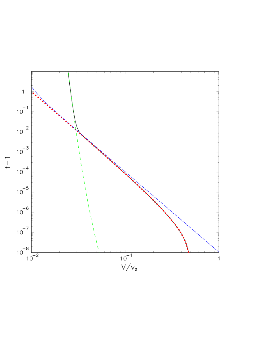
FIG. 3.: Fusion enhancement due to nuclear motion inside a H atom. we present the numerical evaluation of eq.(24) (full line), the approximations of eq.(12) (dotdashed) and of eq.(26) (dotted), the low velocity limit eq.(34) (dashed).

REFERENCES

- [1] C.E. Rolfs and W.S. Rodney, “Cauldrons in the Cosmos”, The University of Chicago Press, Chicago 1988.
- [2] G.Fiorentini, R.W. Kavanagh and C.E. Rolfs, Z.Phys. A 350 (1995)289
- [3] R. Bonetti et al. (LUNA coll.), Phys. Rev. Lett. 82 (1999) 5205
- [4] H.J. Assenbaum , K. Langanke and C.E. Rolfs, Z. Phys. A 327 (1987) 461.
- [5] L. Bracci et al. Nucl. Phys A 513 (1990) 316.
- [6] F. Strieder et al., Naturwissenschaften 88 (2001) 461.
- [7] F. Raiola et al., Eur. Phys. J. A 13 (2002) 377 and Phys. Lett. B (in press).
- [8] L. Bracci, G. Fiorentini and G. Mezzorani Proc. of TAUP 1989, Aquila, Italy, Sep 25-28.
- [9] T.D. Shoppa et al., Phys. Rev C 48 (1993) 837.
- [10] S. Degl’Innocenti and G. Fiorentini, Astron. Astrophys. 284 (1994) 300.
- [11] A.B. Balantekin, C.A. Bertulani and M.S. Hussein, Nucl.Phys. A 627 (1997) 324.
- [12] U. Greife et al. Z. Phys. A 351 (1995) 107
- [13] M. Aliotta et al. Nucl.Phys. A 690 (2001) 790.
- [14] M. Junker et al., Phys. Rev. C 57 (1998) 2700.
- [15] S. Engstler et al. Z. Phys. A 342 (1992) 471.
- [16] A. Musumarra et al. Phys. Rev. C 64 (2001) 068801.
- [17] M. Lattuada et al., Ap. J. 562 (2001) 1076.
- [18] D. Zahnow et al., Z. Phys. A 359 (1997) 211.
- [19] C. Angulo et al., Z. Phys. A 345 (1993) 231.