Mining Weak Lensing Surveys

Abstract

We present a survey of the cosmological applications of the next generation of weak lensing surveys, paying special attention to the computational challenges presented by the number of galaxies, $N_{gal}\sim$ 10⁵. We focus on optimal methods with no pixelization and derive a multigrid $P^{3}M$ algorithm that performs the relevant computations in $O(N_{gal}\log N_{gal})$ time. We test the algorithm by studying three applications of weak lensing surveys - convergence map reconstruction, cluster detection and $E$ and $B$ power spectrum estimation using realistic $1^{\circ}\times 1^{\circ}$ simulations derived from N-body simulations. The map reconstruction is able to reconstruct large scale features without artifacts. Detecting clusters using only weak lensing is difficult because of line of sight contamination and noise, with low completeness if one desires low contamination of the sample. A power spectrum analysis of the convergence field is more promising and we are able to reconstruct the convergence spectrum with no loss of information down to the smallest scales. The numerical methods used here can be applied to other data sets with same $O(N\log N)$ scaling and can be generalised to a sphere.

, ,

1 Introduction

Mapping the matter distribution of the universe is one of the principal aims of cosmology. The traditional approach to this problem has been the use of galaxy surveys, the 2dF Galaxy Redshift Survey [Colless et al. (2001] and the Sloan Digital Sky Survey [York et al. (2000] being the most relevant examples today. However, galaxy surveys only map the luminous matter in the universe; generalising to all forms of matter requires the additional assumption that the luminous matter faithfully traces the total matter distribution. On the other hand, weak lensing, or the coherent distortion of the shapes of background galaxies by intervening matter, requires no such assumption and is emerging as a powerful tool to map the matter in the universe.

The possibility of lensing by large scale structure (LSS) was first pointed out in pioneering work by ?) and has since been theoretically and numerically studied by a number of authors ([Blandford et al. (1991], [Miralda-Escude (1991], [Kaiser (1992], [Bernardeau et al. (1997], [Kaiser (1998], [Jain & Seljak (1997], [Wittman et al. (2000], [Jain et al. (2000], [Wittman et al. (2000]). However, detecting this “cosmic shear” had to wait for advances in imaging technology and has only recently become possible. There now are a number of detections ([Bacon et al. (2000], [Van Waerbeke et al. (2000], [Rhodes et al. (2001], [Hoekstra et al. (2002]) by various groups and with more observations in progress or planned, this number will continue to grow. The next generation of lensing observations such as the NOAO deep field, the CFHT legacy survey and the Deep Lens Survey will go beyond simply detecting cosmic shear but will map it over large areas of the sky. Such large scale surveys will herald in an era of precision cosmology for weak lensing. At the same time, these surveys bring with them the same computational challenges that current CMB experiments and galaxy surveys are facing. The number of background galaxies is $N_{gal}\sim$ 10⁵ to 10⁶, making any brute force approach prohibitively expensive. Analysing these surveys therefore requires the development of algorithms that make the problem computationally tractable. Furthermore, the algorithms must be able to handle aspects of real data including noise, incomplete sampling, arbitrary cuts and so on.

This work has two principal goals; the first is the development of an algorithm that solves the computational challenges of large $N$ surveys, where $N$ can be number of galaxies or just pixelized intensity (as for the CMB). We then test this algorithm (described in detail in the Appendix) on various applications of weak lensing surveys using simulated data. The paper therefore serves the dual purpose of being a test of our algorithm as well as a survey of the potential of weak lensing surveys in cosmology.

We focus on three applications of weak lensing that we believe are the most interesting for cosmology. The first of these, reconstructing the matter distribution, is the basic goal of large lensing surveys. Lensing measures the integrated line of sight matter distribution, or the convergence ($\kappa$) map. Since this reconstruction includes all matter, luminous and dark, such a map gives us a glimpse of the true distribution of matter in the universe. Such maps could also be combined with the high quality imaging data of the lensing survey to understand the relationship between luminous and dark matter. Weak lensing reconstructions have been considered under two broad contexts, cluster mass reconstructions ([Kaiser & Squires (1993], [Kaiser et al. (1995], [Seitz & Schneider (1995]) and LSS reconstructions [Seljak (1998]. Since the surveys we are considering in this paper are large field surveys, we will focus on methods for the latter, including effects of non uniform sampling, irregular boundaries and noise.

The next scales of interest are the largest gravitationally bound systems in the universe, clusters of galaxies. As clusters are the rarest and most massive of all structures, they provide a sensitive probe of structure formation and the initial conditions of the universe. One such test is the number density of clusters [Bahcall & Fan (1998] as a function of mass and redshift, which depends sensitively both on the total matter in the universe as well as the presence of dark energy and its properties. In order to use such tests, one needs to have a large catalogue of clusters, with well defined selection criteria and completeness fractions. One approach is to use large photometric or spectroscopic surveys of galaxies [White & Kochanek (2001] to construct such catalogues; lensing provides us with an alternative approach ([Hennawi et al. (2001], [White et al. (2001]). An advantage to lensing is that it detects all massive structures, whether they are luminous or not, while other methods assume the presence of luminous matter. Since theory predicts the total number of such objects, lensing allows for the most direct comparison to predictions. Also, any possible existence of “dark clusters” (e.g. [Miralles et al. (2002]) would bias the latter methods, while lensing surveys would be unaffected. However, lensing has its own disadvantages that must be understood, if it is to be reliably used.

This paper develops a method to detect clusters in lensing surveys, as well as addressing the theoretical limitations of lensing for cluster searches. It then characterises the completeness and reliability (defined below) of such surveys. We also examine the potential of such surveys to constrain the profile of the dark matter haloes associated with such clusters. This work parallels and extends the work in ?), although we use different methods.

Finally, we address the measurement of the convergence power spectrum. The power spectrum is one of a host of statistics that can be measured, but it has emerged as the statistic of choice for cosmology, since many models predict a gaussian random field distribution on large scales, for which the power spectrum contains all the information. Also, the power spectrum has a natural interpretation from linear structure formation, and therefore is a powerful probe of cosmology, especially in conjuction with other astrophysical measurements ([Jain & Seljak (1997], [Kaiser (1998], [Hu & Tegmark (1999]). The techniques for estimating the power spectrum are similar to those already employed in CMB and galaxy redshift surveys. Here we adapt them to weak lensing.

The paper is organised as follows: We start by describing the features of our algorithm. In $\S 3$, we review the basic formalism of weak lensing, while $\S 4$ describes the simulations used in the paper. We then examine each of our chosen weak lensing applications, image reconstructions ($\S 5$), cluster detections ($\S 6$), and power spectrum estimation ($\S 7$ ). We conclude in $\S 8$. The numerical algorithms used in this paper are described in the Appendix.

2 The Algorithm: Features

As mentioned in the introduction, large weak lensing surveys have the same computational challenges that the next generation of CMB and galaxy survey analyses will face. Maximizing the weak lensing signal involves a high number density of background galaxies distributed over large areas of the sky, implying $N_{gal}\geq$ 100,000 galaxies. All the algorithms described in this paper are written in terms of matrix operations, and the computational challenge is in implementing these $N_{gal}\times N_{gal}$ matrix operations efficiently. The goal of this paper is to show that the challenge is tractable.

The actual numerical method is described in the Appendix; we discuss the various features of the algorithm here.

1. The algorithm works in real space: There are a number of reasons why a real space algorithm is preferable to a harmonic space approach:

   1. The noise properties of data are typically trivially representable in real space.

   2. Real data is not uniform, but involves a number of cuts that arise from bad data, star removal, cosmic ray subtraction etc. In real space, these cuts are trivially included. In harmonic space, these cuts would introduce artifacts due to the non uniformity of coverage, and these are generically difficult to correct for.

   3. Since we do not work directly with Fourier modes there is no need to impose periodic boundary conditions. Thus, there are no issues associated with aliasing of power from the modes on the scale of the survey.

2. There is no pixelisation required: A particularly simple solution to the computational challenges of large data sets is to pixelise the data if possible. There are a number of methods to do this, and one can choose pixels that maximize the signal given a fixed number of pixels. Pixelisation however does involve some degree of data loss at all scales, and no information is preserved below the pixel scale. While this may be acceptable for image reconstruction and power spectrum measurements on large scales, it is undesirable for cluster searches, where small scale information is essential. Furthermore, pixelisation is particularly problematic if the survey geometry is complicated.

3. The time complexity is $N_{gal}\log N_{gal}$ : We have tested our algorithm in the range $N_{gal}=$ 30,000 to 180,000 using a single processor on a workstation. Within this range, the computational time scales (effectively) linearly with the number of galaxies; the processing time ranged from a few minutes for the image reconstructions and halo searches, to a few hours for the Fisher matrix estimation. We also note that the algorithms in this paper, especially the power spectrum estimation, are readily parallelized.

4. The algorithm is generalisable : The algorithm does not use any properties that are unique to weak lensing; most of the methods described here have either been borrowed from other applications, or else are trivially generalisable. Consequently, this algorithm can be used in other applications where large $N$ is a computational restriction.

3 Lensing Formalism

Let us begin by briefly reviewing the basic formalism of weak lensing to establish notation and our conventions. The reader is referred to ?) for more details; our treatment closely parallels the discussion in ?).

The gravitational deflection of light can be described as a mapping between a source (S) and image (I) plane. The mapping can be written as

$$\delta x_{i}^{S}=A_{ij}\,\delta x_{j}^{I}\,\,,$$ (1)

where $\mathbf{\delta x}$ is the displacement vector between two points on a given plane. In the weak lensing regime, the mapping has the form

$$A_{ij}=(1-\kappa)\delta_{ij}-\gamma_{1}\sigma_{3}-\gamma_{2}\sigma_{1}\,\,,$$ (2)

where $\sigma_{i}$ are the Pauli matrices, $\kappa$ is the convergence, and $\gamma$ is the two component shear. Naively, one might expect that this mapping depends on three independent parameters. However, the three components of $A_{ij}$ are not independent; the relation between them most easily expressed in Fourier space (we will assume a small enough patch of sky in this paper to ignore curvature effects),

$$\gamma_{1}({\mathbf{l}})=\kappa({\mathbf{l}})\,\cos(2\phi_{{\mathbf{l}}})\,\,\,\,\,\,;\,\,\,\gamma_{2}({\mathbf{l}})=\kappa({\mathbf{l}})\,\sin(2\phi_{{\mathbf{l}}})\,\,,$$ (3)

where $\phi_{{\mathbf{l}}}$ is the direction of the ${\mathbf{l}}$ mode. Within the weak lensing approximation, the expectation value of the ellipticity is proportional to the shear. The proportionality constant depends on the definition of the ellipticity; we adopt

$$\langle e\rangle=\gamma\,\,.$$ (4)

We now compute the various lensing two point statistics. To do so, we Fourier decompose the shear field into the so-called $E$ and $B$ modes,

$$\gamma_{1}(\mathbf{\hat{n}})=\int\,\frac{d^{2}l}{(2\pi)^{2}}\,[E({\mathbf{l}})\cos(2\phi_{{\mathbf{l}}})-B({\mathbf{l}})\sin(2\phi_{{\mathbf{l}}})]\,e^{i{\mathbf{l}}.\mathbf{\hat{n}}}$$

$$\gamma_{2}(\mathbf{\hat{n}})=\int\,\frac{d^{2}l}{(2\pi)^{2}}\,[E({\mathbf{l}})\cos(2\phi_{{\mathbf{l}}})+B({\mathbf{l}})\sin(2\phi_{{\mathbf{l}}})]\,e^{i{\mathbf{l}}.\mathbf{\hat{n}}}$$ (5)

The two point statistics of these quantities are specified by their power spectra,

$$\langle\,E({\mathbf{l}})\,E({\mathbf{l}}^{\prime})\,\rangle=(2\pi)^{2}\delta({\mathbf{l}}-{\mathbf{l}}^{\prime})\,P^{EE}_{l}$$

$$\langle\,B({\mathbf{l}})\,B({\mathbf{l}}^{\prime})\,\rangle=(2\pi)^{2}\delta({\mathbf{l}}-{\mathbf{l}}^{\prime})\,P^{BB}_{l}$$

$$\langle\,E({\mathbf{l}})\,B({\mathbf{l}}^{\prime})\,\rangle=(2\pi)^{2}\delta({\mathbf{l}}-{\mathbf{l}}^{\prime})\,P^{EB}_{l}\,\,.$$ (6)

We note that weak lensing by density perturbations only produces $E$ modes, while shot noise and systematic effects can produce both. In terms of power spectra, $P^{EE}_{l}=P^{\kappa\kappa}_{l}\,,\,P^{EB}_{l}=P^{BB}_{l}=0$ for weak lensing, while $P^{EE}_{l}=P^{BB}_{l}\,,\,P^{EB}_{l}=0$ for shot noise. Systematic effects can produce all three power spectra. For the rest of this paper, we will ignore $P^{EB}_{l}$ since it is parity violating; we refer to $P^{EE}_{l}=P^{\kappa\kappa}_{l}$ as the $E$ mode power, while $P^{BB}_{l}$ is the $B$ mode power.

Using the above expectation values and standard trigonometric and Fourier identities, we calculate the various covariance matrices,

1. $$S^{\gamma\gamma}_{(ij)(ab)}=\langle\gamma_{ia}\gamma_{jb}\rangle=\int\,\frac{l\,dl}{4\pi}\,\sum_{X=\epsilon\epsilon,\beta\beta}\,P_{l}^{X}I^{X}_{ab}\,\,,$$ (7)

   with

   $$I^{\epsilon\epsilon}_{ab}=\left[\begin{array}[]{cc}J_{0}+c_{4}J_{4}&s_{4}J_{4}\\ s_{4}J_{4}&J_{0}-c_{4}J_{4}\end{array}\right]$$ (10)

   $$I^{\beta\beta}_{ab}=\left[\begin{array}[]{cc}J_{0}-c_{4}J_{4}&-s_{4}J_{4}\\ -s_{4}J_{4}&J_{0}+c_{4}J_{4}\end{array}\right]\,\,.$$ (13)

2. $$S^{\kappa\gamma}_{(ij)(a)}=\int\,\frac{l\,dl}{4\pi}\,P^{\kappa\kappa}_{l}I_{a}\,\,,$$ (14)

   with

   $$I_{a}=(\,-2c_{2}J_{2}\,,\,-2s_{2}J_{2}\,)\,\,.$$ (15)

3. $$S^{\kappa\kappa}_{ij}=\int\,\frac{l\,dl}{4\pi}\,P^{\kappa\kappa}_{l}J_{0}\,\,.$$ (16)

For convenience, we have introduced the shorthand notation $c_{n}=\cos(n\phi),\,s_{n}=\sin(n\phi),\,J_{n}=J_{n}(l\theta)$. The displacement vector between two points $(i,j)$ is described in polar coordinates by $(\theta,\phi)$; the components of the shear are $(a,b)$. We will often omit the superscripts for notational simplicity when referring to these matrices if they are implicit in the context.

4 Simulations

Parameters	Value
$\Omega_{M}$	0.3
$\Omega_{\Lambda}$	0.7
$\sigma_{8}$	0.9
h	0.7
Boxsize	239.5 Mpc/h
Particle Mass	$6.86\times 10^{10}$ $M_{\odot}$/h

Table 1: The cosmological parameters used in the N-body simulations.

The simulated convergence maps used in this paper are derived from the Virgo N-body simulations [Jenkins et al. (1998], run at the Edinburgh Parallel Computing Center and the Computing Centre of the Max Planck Society at Garching. These simulations use a parallel AP³M code ([Couchman et al. (1995],[Pearce & Couchman (1997]) to evolve 256³ particles from z=50 to z=0. The cosmological parameters used in the simulation are in Table  1. The dark matter distribution is then projected onto a series of planes in the redshift range z=2 to z=0. Dark matter haloes with a mass greater than $10^{14}$ M_⊙ are identified with a FOF group finder with b = 0.2, forming the halo catalogue we use in the rest of the paper.

We compute the convergence map from these planes by using discrete multiple plane lensing [Schneider et al. (1992],

$$\kappa=\frac{3H_{0}^{2}}{2}\Omega_{M}\sum_{i=1}^{N}g_{i}\,\frac{\delta_{i}}{a_{i}}\,\Delta\chi_{i}\,\,,$$ (17)

where $\delta_{i}$ is the density perturbation at plane i and $g_{i}$ is the geometrical distance ratio, given by

$$g(\chi,\chi^{\prime})=\frac{r(\chi^{\prime})r(\chi-\chi^{\prime})}{r(\chi)}\,\,,$$ (18)

with $\chi$ the comoving distance and $r(\chi)=\sin_{K}(\chi)$ the usual curvature distance. Two sets of convergence maps are created, 3.5${}^{\circ}\times$ 3.5^∘ maps assuming all the sources are at z=1 and 2${}^{\circ}\times$ 2^∘ maps using the redshift distribution,

$$n(z)\propto z^{2}\exp(-z/z_{0})\,\,\,,z_{0}=0.4\,\,,$$ (19)

to weight the planes in the sum. A representative $1^{\circ}\times 1^{\circ}$ subsection is shown in Fig. 1. In order to create “independent” maps, the origin of the planes is randomly chosen and we restrict ourselves to using $1^{\circ}\times 1^{\circ}$ subsections to create the galaxy catalogues. While the maps are independent on small scales, this breaks down at larger scales, which manifests itself in the high precision numerical experiments of Sec. 6.

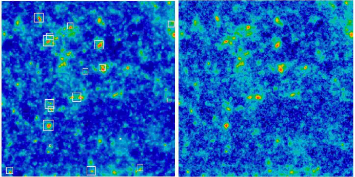
Figure 1: Left: A simulated $1^{\circ}\times 1^{\circ}$ $\kappa$ map, assuming all the sources are at z=1. The map was created using the method described in the text. Haloes with masses greater than 10¹⁴ M_⊙ are marked by squares with the sizes scaled by $\kappa/\Sigma_{crit}$, where $\Sigma_{crit}=\frac{c^{2}}{4\pi G}\frac{D_{s}}{D_{l}D_{ls}}$ and $D_{s}$, $D_{l}$, $D_{ls}$ are the angular diameter distances to the lens, source and between them, respectively. The scale is between -0.06 and 0.26. Right: A WF reconstruction, assuming a background density of n=25 galaxies/arcmin² and an unrealistically small intrinsic scatter in the ellipticities of $\sigma_{int}=0.4/100$.

In order to generate galaxy catalogues, we create shear maps by Fourier transforming the $\kappa$ maps and using Eq. 3. In order to eliminate artifacts from the periodic boundary conditions of the FFT, only the central $1^{\circ}\times 1^{\circ}$ of the shear map is used. We randomly assign galaxies positions, and bilinearly interpolate the shear map and use Eq. 4 to compute their ellipticities. In addition, each galaxy is given a random ellipticity drawn from a Gaussian distribution with $\sigma=0.4$. For the rest of the paper, we refer to the intrinsic ellipticities of galaxies as “noise”. In general, the noise would also contain measurement errors, but we do not simulate these. Note that our method simulates the effect of non-uniform coverage due to the clustering of background sources, although we limit ourselves to Poisson clustering. Table 2 summarizes the different catalogues used in the various sections of the paper.

Section	n	z distribution
Image Reconstruction	10,25,50	yes
Clusters	25,50,100	yes
Power Spectrum	25	no

Table 2: The table summarizes the types of galaxy catalogues used in various sections of the paper. The background density of galaxies (per arcminute²) is given by n, while the third column indicates whether a redshift distribution of the sources was considered or not.

5 Image Reconstruction

One of the basic aims of a weak lensing survey is the reconstruction of the 2D convergence field. A particularly simple nonparametric method for this is Wiener Filtering (WF) [Seljak (1998]. In the case that the data are gaussian distributed, the WF estimator coincides with the maximum posterior probability estimator [Zaroubi et al. (1995] and is therefore, optimal. Even when the data are not gaussian, this estimator still minimizes the variance (as defined below) among all linear estimators; however, it is no longer guaranteed to be optimal. For LSS reconstructions, the deviations from gaussianity on large scales are expected to be small, and so WF is, in an appropriate sense, the best that one can do.

5.1 Theory and Implementation

To derive the estimator, let us organise the ellipticities of N galaxies into a 2N - vector, $\mathbf{e}$. The estimator for the convergence $\mathbf{\kappa}$, at M points can be written as $\mathbf{\hat{\kappa}=\Phi e}$. We wish to minimize the variance,

$$\langle(\mathbf{\kappa-\Phi e})^{t}(\mathbf{\kappa-\Phi e})\rangle$$ (20)

with respect to $\mathbf{\Phi}$. This gives

$${\mathbf{\Phi}}=\langle\mathbf{\kappa e^{t}}\rangle\langle\mathbf{ee^{t}}\rangle^{-1}=S^{\kappa\gamma}(S^{\gamma\gamma}+N)^{-1}$$ (21)

where $S^{ab}$ are the covariance matrices of Sec. 2, and $N$ is the noise covariance matrix. We note that $S^{\gamma\gamma}+N$ is a 2N $\times$ 2N matrix while $S^{\kappa\gamma}$ is an M $\times$ 2N matrix.

In addition, it is essential to generate an error estimate for the reconstruction. We do this by generating mock catalogues created by randomizing the galaxies’ ellipticities and reconstructing the $\kappa$ map for each of these catalogues. The variance over $N_{MC}$ (=200 in this paper) maps is a measure of the error of the reconstructed convergence field. It is important to note that in generating the mock catalogues, the galaxy positions are not altered, thereby explicitly taking into account the non-uniform (here Poisson) sampling of the data.

Using WF requires knowing the exact power spectrum (in the covariance matrices) for it to be optimal. For this one can just use the estimate of the power spectrum from the data using the methods of Sec. 6 [Seljak (1998]. However, empirical tests demonstrate that the reconstruction is relatively insensitive to the power spectrum used if it is roughly approximates the true one, even though the estimator is no longer strictly optimal.

Finally, on the implementation of this algorithm and others in the paper; first, it is not necessary to estimate $\kappa$ at the positions of the galaxies. Indeed, it is more useful to estimate it on a uniform grid; all the figures in this paper are reconstructions on a 256² or 512² grid. Second, while the estimator is theoretically simple, implementating the required matrix operations numerically for $10^{5}$ galaxies and greater, is more of a challenge. There are a number of possible solutions to this; we refer the reader to the appendix for our implementation.

5.2 Results

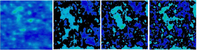
Figure 2: On the left a filtered version of the original map is shown, using a WF appropriate for 3rd panel. The right three panels show WF reconstructions of the $\kappa$ field of Fig. 1, where only those pixels where the measured signal exceeds the noise are shown. Bright (blue) are overdensities, dark (blue) underdensities, while black are pixels where signal is below noise.The density of background galaxies is 10, 25, 50 galaxies/arcmin from left to right, respectively. The intrinsic scatter in the ellipticities is $\sigma_{int}=0.4$. The colour scale is identical to that in Fig. 1.

Figure 3: The power spectra for the WF reconstructions. The continuous [red] line is the power spectrum of the original $\kappa$ map, while the straight dashed [black] line is the noise power spectrum assuming n=25 galaxies/arcmin². The dotted [blue] line is the power spectrum of the reconstruction in Fig.1, while the dashed lines are the power spectra from Fig. 2 (starting from bottom to top, n=10,25,50 galaxies/arcmin²).

The WF reconstructions of the field (Fig.1) for a variety of background densities of galaxies and realistic noise are in Fig. 2, while Fig. 1 shows the reconstruction in the case where the noise has been reduced by a factor of 100. The reconstructions resemble smoothed versions of the original map. This can be understood by considering the WF operator in Fourier space assuming diagonal noise. In Fourier space, the covariance matrices are diagonal with $S^{\kappa\gamma}\sim S^{\gamma\gamma}\sim P^{\kappa\kappa}_{l}$. The WF operator then simply weights each Fourier mode by $P^{\kappa\kappa}_{l}/(P^{\kappa\kappa}_{l}+\hat{\sigma}^{2})$, where $\hat{\sigma}^{2}$ is the amplitude of the noise power spectrum; i.e. every mode is simply weighted by signal/(signal+noise). Considering Fig.3, we see that the principal effect of the WF is to act as a low pass filter, removing modes greater than $l\sim$ 1000. Reducing the level of the noise increases the cutoff frequency of this low pass filter, as can be seen both from the images as well as the power spectra.

The advantages of implementing the WF in real space are evident from the lack of artifacts at the edges of the reconstructions. The presence of an edge is irrelevant to a real space algorithm, and it correctly reconstructs structures at the edge of a field. This is not true for harmonic space approaches which are sensitive to the entire field, and generically produce artifacts at edges.

For completeness, we also considered the reconstructions of fields assuming a redshift distribution of sources and verified that within our implementation of the redshift distribution, there is no effect on the reconstruction. This will continue to be true for more realistic implementations of the redshift distribution except in the limit of sparse sampling (low number of background galaxies). However, WF has only limited value in the sparse sampling limit as is evident from the panels of Fig.2.

6 Clusters

We turn to the construction and characterization of halo catalogues from weak lensing data. Although weak lensing, being sensitive only to the lensing mass, would appear to be the ideal method for constructing such catalogues, it has its own theoretical limitations. We examine these first, then turn to the construction of an optimal filter to detect clusters, and test it. Finally, we address the issue of constraining cluster profiles from weak lensing data.

6.1 Theoretical Estimates

Figure 4: A histogram showing the fraction of haloes with ratio of $M_{lens}/M_{true}$from 200 realizations. The lensing mass was computed by directly summing the $\kappa$ map upto 0.25 $\times$ [dashed/magenta], 0.5 $\times$ [dotted/blue], 1.0 $\times$ [solid/red] the virial radius, $r_{vir}$, and multiplying with $\Sigma_{\rm crit}$ assuming cluster redshift is known. The halo finder mass is scaled assuming an isothermal profile.

Figure 5: The same as Fig. 4 except only 50 realizations were considered and line of sight contamination was removed.

In order to understand the limitations of weak lensing halo searches, we measure the expected signal from our catalogue of dark matter haloes, with no noise added. We define the signal as the ratio $M_{est}/M_{true}$, where $M_{est}$ is the lensing mass estimated from the convergence map, while $M_{true}$ is the halo finder mass. The lensing mass is estimated by integrating $\kappa$ outward from the halo centre upto a fixed fraction of the virial radius, while the halo mass is determined by scaling the halo finder mass assuming an isothermal density profile. The results are shown in Fig. 4. The slight trend in the mass ratio decreasing with radius is a result of clusters being steeper than isothermal in the outer parts of the cluster, such as in NFW profile.

A feature of this plot is the presence of negative masses, i.e. approximately 5% of the haloes are undetectable. These negative masses result from the fact that lensing measures the line of sight integrated mass; low mass haloes can therefore be masked by underdensities. The converse, low mass haloes being masked by heavier haloes, also occurs and is responsible for the long tail of Fig. 4. Removing line of sight contamination (Fig. 5) by considering each lensing plane individually (Eq. 17) removes both the negative masses and the tail, verifying our interpretation. This figure shows that the lensing masses are systematically greater than the halo finder masses. This is the combination of two effects; the true profiles are not isothermal, and so using an isothermal profile to scale the halo finder masses will underestimate the mass. Also, the lensing masses are 2D projected masses, while the halo finder measures the 3D distribution.

Another related concern are filaments oriented along the line of sight that could masquerade as haloes. In order to determine the degree of contamination, we consider all pixels in our $\kappa$ maps that exceed a particular threshold (we tried a few different thresholds, but our results were insensitive to the particular choice). We then compute the distance, $\Delta\theta$, between the pixel and the closest halo. This is a measure of the correlation between the $\kappa$ overdensities and the haloes. We find that all but a negligible fraction of overdensities did not correspond ($\Delta\theta>1$ arcmin) to real haloes, implying that contamination due to filaments is insignificant.

6.2 Cluster Detection: matched filters

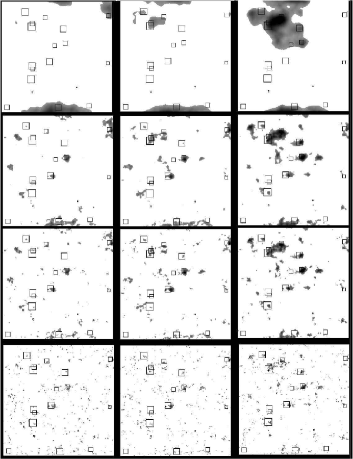
Figure 6: Cluster detections for a variety of scale lengths and galaxy densities, using a threshold of $\sigma=2$. The darkness is proportional to the significance of the detection, saturating for $\sigma>5$. Haloes with masses over $10^{14}M_{\odot}$ are marked by the boxes with the size of the box dependent on the expected signal. The columns are different background galaxy densities, n=25,50,100 galaxies/arcmin² from left to right. The rows are different scale lengths, $\theta_{s}$ = 5.0,1.0,0.5 and 0.1 arcminutes from top to bottom. The realizations here did not include a redshift distribution.

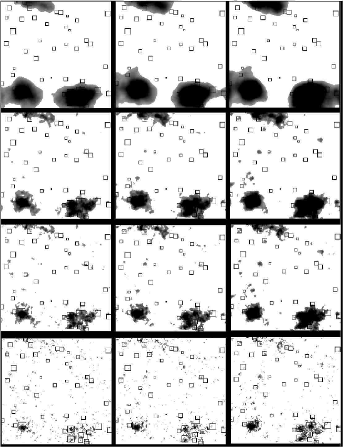
Figure 7: Same as Fig. 6 except that a redshift distribution was used in the realizations.

The problem of halo detection can be formally stated as follows - given an input signal with a spatial distribution $f({\mathbf{x}})$ and amplitude $A$, the measured signal can be written as

$$f^{\prime}({\mathbf{x}})=A\,f({\mathbf{x}})+N({\mathbf{x}})$$ (22)

where $N({\mathbf{x}})$ is the noise. Assuming that the noise has zero mean and and its statistical properties are spatially independent, the minimum variance estimator, $\Phi$, has the form (in Fourier space) [Haehnelt & Tegmark (1996],

$$\Phi({\mathbf{k}})\propto\frac{f(\mathbf{k})}{N({\mathbf{k}})}\,\,.$$ (23)

Specializing to the case of lensing, the estimator is given by

$$\Phi\propto\frac{S^{\prime\kappa\gamma}}{N}\,\,.$$ (24)

The normalization is usually determined by requiring that it be unbiased. However, since we are interested in the ratio of the signal to the noise, the normalization cancels and we leave it arbitrary. The signal matrix, $S^{\prime\kappa\gamma}$, has the same form as the unprimed matrix of equation 14, except that the input power spectrum is replaced by the Fourier transform of the halo profile.

We now describe our halo detection algorithm. We start by convolving the shear map with the matched filter; in practice, this involves multiplying the data (organised into a vector) by the matrix in Eq. 24. Let us denote this convolved map by $\tilde{\gamma}({\mathbf{x}})$ - we must now determine whether the value of $\tilde{\gamma}$ at a given point determines a cluster or not. In order to do this, we start with the null hypothesis, i.e. there is no halo at ${\mathbf{x}}$ and ask whether $\tilde{\gamma}({\mathbf{x}})$ is consistent with this. Under the null hypothesis, the expectation value of $\tilde{\gamma}({\mathbf{x}})$ is zero with variance $\sigma^{2}$. We define a cluster detection if $\tilde{\gamma}({\mathbf{x}})>n\sigma$, where $n$ is some chosen threshold. We compute $\sigma$ as in the previous section, by randomising the galaxy ellipticities while keeping their positions fixed to create 200 noise maps, and measuring the variance of the resulting convolved maps.

We must emphasize a number of points at this stage. The first is that for any given threshold, we expect to have points not associated with a halo to have $\tilde{\gamma}({\mathbf{x}})>n\sigma$; this fraction of false detections will decrease with increasing $n$. If the noise is Gaussian, then the fraction is known analytically; however, as we will see in the following sections, the noise is not consistent with being Gaussian. Indeed, the principal sources of noise come from extraneous structures not associated with the halo; these structures do not constitute a Gaussian random field. It is however possible to calibrate the expected false fraction from simulations and include it in theoretical analyses. We also re-emphasize that when computing the variance, it is important to leave the galaxy positions unchanged and only randomise the ellipticities. Only by leaving the galaxies’ positions unchanged will the signal, which is dependent on the distribution of background galaxies, be properly estimated.

The cluster profile is still a free parameter. A particularly simple choice is the singular isothermal sphere, which in projection is $\propto\theta^{-1}$. This choice has the disadvantage of excessively weighting the outer parts of the halo (the integrated profile is logarithmically divergent), which are both noise dominated and contaminated by external structures. Numerical experiments with it also verify that it is suboptimal.

A simulation motivated choice is the NFW profile in projection ([Navarro et al. (1997], [Bartelmann (1996]). However, the NFW profile has a $r^{-1}$ inner cusp, which is not resolved by our simulations. Considering the NFW profile, convolved with the simulation pixels, suggests a profile of the form [White & Kochanek (2001],

$$f(\theta)=\frac{1}{(1+\theta/\theta_{s})^{2}}\,\,,$$ (25)

where $\theta$ measures angular seperation on the sky. This profile has the same aysmptotic $\theta^{-2}$ behaviour of the NFW profile; within the scale radius $\theta_{s}$, it possesses a core. Note that we have introduced an angular scale into the filter, and that there is no way to theoretically choose this scale for all clusters, since they will be at different distances. When analyzing real data one may of course choose a projected NFW profile instead, which however still has a physical scale that cannot correspond to a single angular scale. We resolve this problem by simply using a series of scale radii to perform the reconstructions.

The results for $\theta_{s}=$ 5.0, 1.0, 0.5 and 0.1 arcminutes are shown in Figs. 6 and 7. As is evident from the figures, the scale radius corresponds to a smoothing scale. A larger scaling length results in fewer false detections, but tends to coalesce seperate haloes into single structures and misses a greater fraction of clusters. Decreasing the scale radius resolves seperate structures better, but is also more susceptible to noise and extraneous structures, as can be seen from the number of detected structures that do not correspond to haloes.

6.3 Completeness/Reliability

Figure 8: The completeness fraction for different thresholds and scale lengths, computed from 200 realizations, with a background density of n = 25 galaxies/arcmin². The panels are labelled by the scale length in arcminutes. The solid [black], dotted [red] and dashed [blue] lines represent thresholds of $\sigma=2,3$ and $4$ respectively. The bin size is 0.05 $r_{vir}$, implying the central completeness ($r<0.1r_{vir}$) is contained in the first two bins.

Figure 9: Same as Fig. 8 except that a redshift distribution was used in the realizations.

It is useful to recall at this stage that we have two lists of data, a list of haloes from the halo finder and a list of pixels whose halo signal was above a certain threshold. There are two obvious questions one can ask - what fraction of haloes have associated pixels, and what fraction of pixels have associated haloes. We define the completeness as the fraction of haloes that have their closest detected pixel a specified distance away from them. Conversely, the reliability is defined as the fraction of pixels that have their closest halo a specified distance away. We note that the natural measure of distance for completeness is in units of the virial radius, whereas the reliability distance is measured as a physical angular distance.

The completeness fractions, for three different thresholds, are shown in Figs. 8 and 9. We make the following observations about these results:

1. As expected, increasing the threshold reduces the completeness fraction. Note however that this happens at 2-3$\sigma$ level, so one cannot choose a high level of significance (thereby rejecting spurious detections with high confidence) and have a high level of completeness at the same time.

2. The width of the completeness distribution is also seen to widen as the scale length decreases. This can be understood heuristically by noting that as the maps become more noise dominated, the point closest to the halo may be unrelated to it, thereby broadening the distribution. A crude modelling of the distribution in the limit of purely random, independently distributed points obtains,

   $$f(x)\propto x\,(1-x^{2})^{n}\,\,;\,x=r/r_{vir}\,\,,$$ (26)

   which, for $n\sim 5$ resembles the distribution for the smallest scale radius. Note however that this is meant to be illustrative, and not a close approximation to the actual distribution.

3. A redshift distribution of the sources decreases the completeness fraction. This is the result of two competing effects - using a redshift distribution allows one to probe a larger volume of space, and one would hope to detect more clusters in that region. On the other hand, the redshift distribution results in a more non uniform signal which reduces the signal.

Figure 10: The reliability fraction for different thresholds and scale lengths. The panels are labelled by the scale length in arcminutes. The solid [black], dotted [red] and dashed [blue] lines represent thresholds of $\sigma=2,3$ and $4$ respectively.

Figure 11: Same as Fig. 10 except that a redshift distribution was used in the realizations.

$\theta$ (arcmin)	$\sigma$ =2	3	4
5.0	0.27	0.20	0.14
1.0	0.23	0.12	0.06
0.5	0.24	0.12	0.05
0.1	0.35	0.22	0.07

Table 3: The fraction of detected pixels that did not have a corresponding halo within 5 arcminutes, as a function of the scale radius, $\theta_{s}$ and the threshold, $\sigma$. For simplicity, we have only shown the figures for simulations without a redshift distribution; the case with a redshift distribution is similar.

The corresponding reliability fractions are shown in Figs. 10 and 11, and the fraction of detected pixels that had no corresponding halo within 5 arcminutes is in Table 3. Note that we have only shown the fractions for the simulations without redshift distributions; including a redshift distribution produces similar results. We note the following:

1. The reliability fraction becomes more peaked as the threshold increases.

2. The above trend becomes more pronounced as the scale radius decreases, implying that a higher threshold is necessary to eliminate noise at these scales. However, the number of detected pixels at both high thresholds and small scales also steeply decreases, again pointing to intermediate scales for optimal cluster detection.

3. Unlike the completeness, the reliability appears to be insensitive to a redshift distribution.

4. Finally, the dropoff near the origin is a purely geometrical effect, due to the fact that the differential area grows linearly with radius.

Figure 12: The completeness fraction (integrated to 0.2 r_vir) as a function of halo mass. The panels are labelled by the scale length in arcminutes. The solid [black], dotted [red] and dashed [blue] lines represent thresholds of $\sigma=2,3$ and $4$ respectively.

Figure 13: Same as Fig. 12 except that a redshift distribution was used in the realizations.

It is also useful to consider completeness as a function of halo mass, we do this in Figs. 12 and 13. The completeness plotted is an integrated quantity - the fraction of haloes that have a detected pixel within 0.2 $r_{vir}$ of them. The completeness is a steep function of halo mass, with the surveys being nearly 100% complete at the high mass end, but less than 5% complete for the lowest masses. The noisy nature of these plots is simply an artifact of the fact that our simulations have few massive haloes.

An important observation to make is that the achieved completeness is significantly lower than what one might have expected theoretically. This discrepancy can be traced back to the assumption of a uniform signal in our theoretical estimates. The Poisson clustering of the background galaxies does not satisfy this assumption; indeed, configurations of background galaxies make certain haloes undetectable. This would be even worse if one included clustering of the background galaxies, and must be taken into account when computing predicted cluster finding efficiency as a function of halo mass.

6.4 Cluster Profiles

Figure 14: The integrated $\kappa$ profile created by stacking clusters in three mass bins, 1-3 $\times$ [dashed/blue], 3-6 $\times$ [dotted/red], $>$ 6 $\times$ [dot-dashed/green] 10¹⁴ M_⊙. The profile is arbitrarily normalized to unity at the virial radius. The solid [black] line is arbitrarily normalized c=4 projected NFW profile shown for comparison.

Figure 15: Same as Fig. 14 except for the tangential shear profile.

Figure 16: The tangential profile for the profile in Eq. 25 with $\theta_{s}$ = 5.0 [solid/black], 1.0 [red/dotted], 0.5 [blue/dashed] and 0.1 arcminutes [dot-dashed/green]. The normalisation has been adjusted to agree with Fig.15, and the virial radius of the cluster has angular size 2.5 arcminutes.

There has been considerable interest recently [Sheldon et al. (2001] in using weak lensing to statistically constrain cluster halo profiles. We examine this by considering both the integrated mass profile (Fig. 14) and the tangential shear profile (Fig. 15). The integrated mass profile is simply given by summing our convergence map with no noise added. For the shear profile, we use our simulated catalogues. The ellipticity of each galaxy is decomposed, relative to the halo center, into a tangential and radial component, which we then average in radial bins to get the profile. Unlike the integrated mass profiles, the shear profiles are estimated in the presence of noise.

We divide clusters into three mass bins, and average the profiles within those bins assuming we know their central positions. This simulates the process of “stacking” clusters with centers known from X-ray or optical data. The profiles are seen to be well constrained for the highest mass bin and poorly constrained at low masses.

We can also compare the measured shear profiles to what one would expect if one assumed a convergence profile of the form in Eq. 25. The expected profiles for the four scale radii we use are shown in Fig.16. As we might have anticipated from the results of the two previous subsections, the best agreement is when $\theta_{s}$ is between 0.5 and 1.0 arcminutes. It is also important to emphasise that the dropoff seen in Fig.15 is an effect of the pixelisation of the map; a similar effect is seen in Fig.16 where the core radius mimics the effects of pixelisation. If clusters had significant cores, then just such an effect would be also physically expected.

7 Power Spectrum Estimation

In this section we consider the measurement of the convergence power spectrum from weak lensing data. The subject of the optimal measurement of the power spectrum from noisy data has received a lot of attention, with regards to the CMB and galaxy redshift surveys, and we will simply import the techniques that have been developed and validated there to weak lensing. It should be emphasized that weak lensing, unlike galaxy redshift surveys, measures the matter power spectrum directly, eliminating the complications of bias.

Since the formalism for optimal weak lensing power spectrum measurement has been discussed in detail elsewhere (see for eg. [Seljak (1998], [Tegmark et al. (1998]), we will limit ourselves to a brief discussion (following the notation in [Padmanabhan et al. (2001]) to establish the formalism we will be using. A similar discussion that uses a different, although related, approach is in ?).

7.1 Theory

Let us parametrize the power spectrum by N_p step functions such that $P(l)=p_{i}$ for $l_{i-1}\leq l\leq l_{i}$, where $i$ ranges from 1 to N_p. We can now arrange the $p_{i}$ into an N_p-vector, ${\mathbf{p}}$. The problem now reduces to estimating ${\mathbf{p}}$ from the data ${\mathbf{x}}$, where ${\mathbf{x}}$ is a 2N vector consisting of the galaxy ellipticities. Define the covariance matrix of the data, $C=S^{\gamma\gamma}+N$ where $S^{\gamma\gamma}$ is the signal covariance matrix (see Sec. 2) while $N$ is the noise matrix. Recall that $N=N_{meas}+N_{int}$ where $N_{meas}$ is the measurement noise, while $N_{int}$ is the intrinsic noise due to galaxy ellipticities. This intrinsic noise is not known a priori and must be estimated from the data, an issue we address at the end of this section.

Since the power spectrum is the sum of step functions, we rewrite the covariance matrix,

$$C=\sum_{i=1}^{N_{p}}p_{i}C_{i}+N=\sum_{i=0}^{N_{p}}C_{i}\,\,,$$ (27)

where $C_{i}=\partial S^{\gamma\gamma}/\partial p_{i}$ for $1\leq i\leq N_{p}$, and we have defined $C_{0}=N$ and introduced a dummy parameter, $p_{0}=1$ for notational convenience.

We now form the minimum variance quadratic estimators ([Hamilton (1997a], [Hamilton (1997b], [Tegmark (1997]),

$$q_{i}=\frac{1}{2}{\mathbf{x}}^{t}C^{-1}C_{i}C^{-1}{\mathbf{x}}$$ (28)

and group them into an N_p+1 vector, ${\mathbf{q}}$. The quadratic estimators have the following properties,

$$\langle{\mathbf{q}}\rangle=F{\mathbf{p}}$$

$$\langle{\mathbf{q}\,q}^{t}\rangle-\langle{\mathbf{q}}\rangle\langle{\mathbf{q}}\rangle^{t}=F$$ (29)

where $F$ is the Fisher information matrix ([Tegmark et al. (1997] and refs. therein),

$$F_{ij}=\frac{1}{2}tr\left[C^{-1}C_{i}C^{-1}C_{j}\right]\,\,\,.$$ (30)

The best estimate of the power spectrum can be written as

$$\mathbf{\hat{p}}=M({\mathbf{q}}-{\mathbf{b}})$$ (31)

where ${\mathbf{b}}=F_{i0}$, and we restrict all indices to run from 1 to N_p. The matrix $M$ is an arbitrary N${}_{p}\times$ N_p matrix with the property that the rows of $MF$ sum to unity and is chosen such that our power spectrum estimates have certain desirable properties. The choices for $M$ that we consider and their properties are listed in Table 4. Note that there is no gain in information in this final step; the information content is the same as what is in the quadratic estimators and the entire Fisher matrix. However, if one only presents the diagonal of the Fisher matrix (eg. errorbars in a plot), then it is important to ensure that the errorbars are uncorrelated (the third choice). Our estimates $\mathbf{\hat{p}}$ now have the following properties,

$$\langle\mathbf{\hat{p}}\rangle=W{\mathbf{p}}=MF{\mathbf{p}}$$

$$\langle\mathbf{\hat{p}\hat{p}}^{t}\rangle-\langle{\mathbf{p}}\rangle\langle{\mathbf{p}}\rangle^{t}=MFM^{t}\,\,,$$ (32)

where we note that the rows of $W$ have the obvious interpretation as window functions.

M	Properties
$(\sum_{j=1}^{N_{p}}F_{ij})^{-1}\,\delta_{ij}$	minimum variance,
	correlated errorbars
$F^{-1}$	anti-correlated errorbars,
	delta function windows
$[\sum_{j=1}^{N_{p}}(F^{1/2})_{ij}]^{-1}(F^{-1/2})_{ij}$	uncorrelated errorbars

Table 4: The various choices for $M$ (Eq. 31) and their properties.

7.1.1 Choosing a prior

In the preceding discussion, we have implicitly assumed a prior power spectrum, and all the properties have rested on this prior being the true power spectrum. This begs the question - how does one choose the prior? Any reasonable guess to the power spectrum works as an initial guess. The power spectrum estimated then can be used as the prior, and the process can be iterated. Several authors ([Bunn (1995], [Padmanabhan et al. (2001] ) have explicitly verified that the choice of prior does not bias the result, and therefore, in practice, only one or two iterations are required.

7.1.2 Measuring the intrinsic ellipticity scatter

The intrinsic scatter in the ellipticities can be estimated by simply computing the r.m.s. value of the ellipticity of the data. This will produce the correct answer so long as the shear correlation length is smaller than the size of the field considered. However, if the scatter is underestimated, then the extra power will manifest itself as excess power in the $E$ and $B$ modes. In order to correct for this, we follow ?) and introduce a shot noise parameter, $p_{noise}$, to the power spectrum, whose contribution to the power spectrum is $C_{noise}=p_{noise}\delta_{ij}$. As with the power spectrum, the excess power measured this way can be corrected in the next iteration.

7.2 Results

Figure 17: The $E$ mode power spectrum, averaged over 200 Gaussian realizations. The [red] triangles show the input power spectrum, while the heavily shaded [black] regions are the same power spectrum convolved through the window functions. The width of the regions are the errors predicted by the Fisher matrix. The lightly shaded [green] regions are the estimated power spectrum, with the widths representing the errors calculated from the realizations.

Figure 18: The same as Fig. 17 except for the $B$ mode power. Note that there was no input power; however, there is power expected in the leftmost band due to leakage of power through the window function.

The Fisher matrix formalism is only exact for Gaussian random fields, and so, in order to test it, we simulate 200 gaussian random convergence fields with a known $E$ mode power spectrum, and no $B$ mode power. Figs. 17 and 18 summarize the results. The triangles are the input power spectrum, while the heavily shaded boxes are the input power spectrum convolved with the window functions. The width of the boxes are given by the Fisher matrix error estimates. The lightly shaded boxes are the measured power spectrum, averaged over 200 realizations, with the width of the box given by the standard deviation over the realizations. If the method is correct, then both the power spectrum and the errors should agree. The agreement is best for the $E$ mode power, where the input power was non-zero. We note that although the input $B$ mode power was zero, we expect to see power measured due to leakage from the $E$ modes through the window functions. This is significant only for the leftmost band, that probes scales larger than the survey. We observe that the remaining $B$ mode power is consistent with zero, as expected.

Figure 19: Same as Fig. 17 except that the 200 realizations were drawn from N-body simulations instead.

Figure 20: Same as Fig. 18 except that the 200 realizations were drawn from N-body simulations instead.

Figs. 19 and 20 show the expected and measured power for 200 realizations drawn from N-body simulations, which allow us to test whether the breakdown of the gaussian approximation biases our results. We find that the Fisher matrix underestimates the true errors in the power spectrum. A similar effect was found by ?). Although this is not a large effect, N-body simulations must be used to calibrate the Fisher matrix errors when using the power spectrum estimates to extract cosmological information. The second observation is the discrepancy between the expected and measured $E$ mode power in the leftmost bands. This is due to the fact that all our realizations were derived from the same N-body simulations, and although we expect the realizations to be independent on small scales, this will break down at large scales. Fig. 17 verifies this expectation. Note that these bands probe scales larger than those simulated; it is interesting that we correctly estimate the power to within a factor of two in these bins.

Figure 21: The measured power spectrum from a single N-body realization using choice 1 of Table 4. The solid lines are the expected power, while the boxes are the expected power with Fisher errors. The points are the deviation of the $B$ mode power from zero, shown by the dashed line.

Figure 22: Same as Fig. 21 except that it uses choice 3 of Table 4.

All of the above results use the third choice of Table 4 for $M$. Figs. 21 and 22 contrast the first and third choices for $M$. As expected, the errorbars for the first are smaller, but are correlated, as compared to the third. The effects of decorrelating are pronounced for the $B$ mode power; the points are randomly distributed above and below zero, while in Fig. 21, they are clearly correlated. We therefore reemphasize the importance of decorrelating points when visually presenting data. We do not present the results for the second choice since the errorbars are too large to be useful in this case. This is a direct result of the fact that the window functions in this case are delta functions.

8 Discussion

Weak lensing is emerging as an important tool in cosmology. One of its principal advantages is that it probes the matter distribution directly, making no assumptions about the dynamical state of the matter. This is desirable both because it eliminates complications of interpretation, but also because it gives us an opportunity to study the physical processes underlying those assumptions.

In this paper, we considered three applications of large weak lensing surveys. We summarise the results here, comparing it to previous work.

8.1 Image Reconstruction

The simplest goal of a weak lensing survey is to produce a map of the distribution of matter in the universe. Wiener filtering provides a simple, and almost optimal reconstruction of the matter distribution, and is our method of choice. An important characteristic of Wiener filtering is that it suppresses power on scales with low signal to noise. For the weak lensing maps we consider here, this scale is at $l\sim 1000$, while there is no power at scales larger than $l\sim 360$, the scale of the survey. This suggests the obvious design strategy of large area surveys to probe large scales, with high background number densities $n\geq 25$ to resolve features on small scales. However, Wiener filtering has limited cosmological applicability because of its inability to resolve smaller structures.

8.2 Cluster Detection

Clusters, as the most extreme structures in the universe, are a sensitive probe of cosmology. Weak lensing has the advantage that it searches for clusters directly as mass enhancements, independent of the presence of luminous matter. However, in order to compare with theoretical predictions, one must, in addition to compiling a catalogue of clusters, understand the selection criteria and the completeness of the catalogue.

A disadvantage of weak lensing is that it measures the projected mass distribution, and is therefore susceptible to contamination from uncorrelated haloes in the line of sight. This is worst for the low mass haloes, since they can be obscured by either more massive haloes or underdensities. More massive haloes are less sensitive to this effect and the theoretical maximum completeness approaches 100%.

The philosophy that we adopt in this paper is that weak lensing cluster searches will be done in conjunction with other measurements such as galaxy, X-ray or Sunyaev-Zel’dovich surveys. One could either imagine using weak lensing to identify candidate clusters and verifying them with follow up measurements, or correlating different measurements to remove false detections. With this in mind, we develop an optimal filter approach to detecting clusters. Detections are defined as those regions where the measured signal to noise ratio exceeds a certain threshold. We then compute the completeness (the number of haloes with a corresponding detection) and the reliability (the number of detections with a corresponding halo). We observe that completeness is strongly dependent on the mass of the cluster; for cluster masses $>$ 6 $\times$ 10¹⁴ M_⊙, our cluster samples were virtually 100% complete independent of the threshold used, implying that one could construct a uncontaminated, yet complete sample, by choosing a high enough threshold. At lower masses, the completeness drops drastically as the threshold in increased. At low thresholds however, the false detection rate rises to $\sim$ 25%. This is a direct result of the fact that our estimator is sensitive to spurious structure masquerading as a halo at low thresholds. We should however note that even for low thresholds, the completeness for low mass haloes is less than 40%.

The optimal filter defines a scale length that physically corresponds to a smoothing scale. Excessive smoothing reduces the number of false detections, since the noise is reduced but it also smooths away or coalesces small sclae structures. As we reduce the smoothing scale, we start to resolve smaller structures but are more susceptible to spurious detections from extraneous structures that don’t belong to any halo. The optimal scale length is $\sim 1^{\prime}$. However, some caution should be exercised when interpreting this value since it may be affected by pixelisation in the N-body maps.

This work parallels a similar study by ?), although we use different methods to detect clusters. ?) use both a simple Gaussian smoothing with a smoothing scale of 1’ - 2’, and aperture mass measures [Schneider (1996] with a scale of 1’-5’ and a signal to noise threshold varying from $S>1$ to $S>5$. As with our methods, the completeness drops with increasing scale radius, with the maximum at $\sim 1^{\prime}$, although ?) do not consider smaller scale lengths. In addition, they conclude that their catalogues are complete for masses $>5\times 10^{14}$ M_⊙, consistent with our results.

An extension of this is the inclusion of a redshift distribution of the background sources. Including this distribution does not qualitatively change any of the trends one observes for, but reduces the overall completeness. The halo catalogues, constructed assuming a redshift distribution, are complete for masses $>8\times 10^{14}$ M_⊙ . This is what one might naively expect - the most massive haloes are unaffected by the redshift distribution, while the signal from the less massive haloes is reduced and a larger fraction of them are missed. The reliability is however unaffected by a redshift distribution, because false detections are due to noise and extraneous structure, and one would not expect those to be affected by a redshift distribution.

There are two cautionary lessons that we draw from this work. The first is that the optimal nature of matched filters is easily affected by deviations from ideality. These are caused here by deviations from circular symmetry due to extended haloes, as well as internal and external substructure. The second is that the completeness of cluster surveys are strongly affected by clustering of the background galaxies. Certain haloes are rendered undetectable by the Poisson clustering of our simulated background galaxies. Real background galaxies are not Poisson distributed, but are correlated, and we expect this to have a worse effect. Therefore, all analyses must take into account the clustering of source galaxies to get a representative measure of the expected completeness of the survey.

We note that we have restricted ourselves here to consider the information from lensing only. However, lensing surveys will produce high resolution multi-colour images of the survey region. One might imagine using both the lensing and imaging data simultaneously to detect clusters; such an approach would naturally reduce the number of false detections. Another advantage to using the imaging data jointly with the lensing is that each complements the other - lensing would identify haloes with no optical counterpart, while optical searches could detect objects with low lensing signals.

8.3 Power Spectrum

The convergence power spectrum is a measure of the clustering of the recent universe, a regime that was accessible until now only to redshift surveys. In contrast with the galaxy power spectrum, the convergence power spectrum is not affected by the complications of biasing, and provides a direct measure of the matter power spectrum.

The formalism for estimating the power spectrum, borrowed from the CMB and galaxy surveys, assumes that the convergence field is Gaussian distributed. While this is not true for the true convergence field on small scales, it is approximately true on the scales that lensing probes. We have explicitly shown, using N-body simulations, that the Gaussian approximation does not bias the estimators. However, the Fisher matrix underestimates the error bars and although this is not a large effect, it means that the error bars must be calibrated against N-body simulations. Our results are similar to those obtained by ?) although our methods differ in details. The main difference is that our method does not pixelise and so extracts all the information from the data.

In concluding, we observe that the methods presented here are not unique in their application to weak lensing. We have used methods developed for analysis of other data sets and adapted them to weak lensing. New numerical solutions presented here may be adapted to other similar problems in cosmology, particularly those where brute force evaluations are prohibitely expensive. In our application we have managed to reduce an instrinsic $O(N^{3})$ numerical problem to $O(N\log N)$. The same methods can be used in other applications, such as the analysis of CMB temperature and polarization anisotropies and galaxy surveys. We expect that both lensing and other areas of cosmology will benefit from the growing synergy in the field.

We would like to thank SISSA, Trieste, where this work was begun, for its hospitality. We thank VIRGO collaboration for making N-body simulations available to the community. We would also like to thank Joe Hennawi, Catherine Heymans, Christopher Hirata, Kevin Huffenberger and David Spergel for useful discussions. N.P. was supported by a Centennial Graduate Fellowship from Princeton University. U.S. is supported by NASA, NSF CAREER, David and Lucille Packard Foundation and Alfred P. Sloan Foundation. U.P. is supported by NSERC grant 72013704. Computing infrastructure was provided in part by the Canada Foundation for Innnovation PScinet alphacluster.

Appendix A Numerical Implementations

An important feature of all the algorithms presented in this paper is that they are explicitly written as linear algebra operations. The basic building block of any implementation is therefore a routine to perform matrix-vector multiplication. Unfortunately, the dimensionality of the vector space, $N$, is given by the number of data points. A naive application of the algorithms yields $N\sim N_{gal}\approx 100,000$ for which straight matrix-vector multiplication, an $N^{2}$ process, becomes computationally impractical.

One can approach this problem in two ways, either by reducing $N$, or by using properties of the matrices that appear to speed up the vector multiplications. The former approach is equivalent to pixelising the data and a number of pixelisation schemes have been suggested, ranging from direct binning to “optimal” Karhunen-Loéve pixelisations of the data.

We propose and implement an approach that is based on the latter approach. We start by observing that all the matrix operations that we require are of the form $C{\mathbf{x}}$ or $C^{-1}{\mathbf{x}}$ where $C$ is a correlation matrix of $\S 3$. The latter operations can be recast as direct matrix-vector multiplications by performing the matrix inversion iteratively (we specify the exact algorithm below). We then observe that the multiplication $C{\mathbf{x}}$ is simply a convolution of the data by the appropriate correlation function, $\zeta$,

$$(C{\mathbf{x}})_{i}=\sum_{j}C_{ij}\,x_{j}=\sum_{j}\zeta({\mathbf{r}}_{i}-{\mathbf{r}}_{j})x_{j}\,\,,$$ (33)

where the last identity follows from the fact that the correlation function only depends on the seperation between the two points. The problem is now explicitly translationally invariant and one can readily apply the Fourier convolution theorem to perform the vector multiplications efficiently. The asymptotic scaling is now $O(N\log N)$ instead of $O(N^{2})$, making $N\sim 10^{5}$ tractable on a workstation.

The careful reader will no doubt point out that the use of Fourier methods requires the data to be uniformly sampled, which our data is not. We solve this problem by resampling the data onto a grid of $N_{grid}\sim 4N_{gal}$ points where the additional factor of 4 comes from the need to zero pad in 2 dimensions. The exact scaling of the algorithm is therefore $N_{grid}\log N_{grid}$. We emphasise that although an auxiliary grid is used, this grid is only an intermediate step which does not impose periodic boundary conditions, and whose discreteness effects can be compensated using multigrid and direct summation methods as described below. Our approach is thus conceptually very different from pixelisation approaches. It is also useful at this stage to point out the obvious analogy between our approach and gravity solvers of PM (particle - mesh) N-body simulations.

While the above approach works well for large scale modes, the pixelisation introduces inaccuracies at scales comparable to the pixel resolution. Our analogy with N-body simulations come to the rescue here; PM simulations have similar inaccuracies on small scales that can be corrected by introducing a direct summation between pairs of particles at small seperations (P³M - particle-particle particle-mesh simulations). We start by splitting the convolution kernel into short and long range pieces,

$$\zeta\,=\,\zeta_{long}+\zeta_{short}\,=\,f(r)\zeta+g(r)\zeta\,\,,$$ (34)

where $f$ and $g$ are filter functions with the properties that

$$g=1\,\,\,(r<r_{min})\,\,\,,$$

$$f=1\,\,\,(r>r_{max})\,\,\,,$$

$$f=0\,\,\,(r<r_{min})\,\,\,,$$

$$g=0\,\,\,(r>r_{max})\,\,\,,$$

$$f+g=1\,\,\,(r_{min}<r<r_{max})\,\,\,,$$ (35)

with the definitions of long and short range are determined by $r_{min}$ and $r_{max}$. The multiplications are now done in two stages; the first is to do the long range piece by the Fourier method described above, while the short range correlations are done by direct summation. Possible filter functions have the form $1-\cos^{2}(\theta)$ in the regime $r_{min}<r<r_{max}$, where $\theta$ is an appropriately scaled length. This form is chosen to minimise the inaccuracies that result from the truncation of the correlation function.

A second scheme to improve the resolution is to use a multi-grid approach. The single-grid scheme described above is only the simplest such implementation. One can trivially generalise it to multiple scales by introducing a series of filters, $f_{i}$. In such implementations, the direct summation is performed only for the shortest range; all other convolutions are done by the Fourier method with the grid becoming coarser for larger scales. Our codes used 3 scales - the innermost scale for direct summation, an intermediate scale with twice the resolution, and a coarse grid for the largest scales.

Note that while the $O(N\log N)$ scaling is dependent on a flat space assumption, it can be generalized to the sphere with no significant loss of efficiency. This is because on a sphere only the coarse grid needs to be done with the slower $O(N_{\rm coarse}^{3/2})$ scaling, while the subsequent grids can still be $O(N_{\rm grid}\log N_{\rm grid})$ as long as the flat sky approximation holds on these grids.

A.1 Matrix Inversions

The problem we focus on is of the form

$${\mathbf{y}}=C{\mathbf{x}}=(S+N){\mathbf{x}}\,\,,$$ (36)

where ${\mathbf{y}}$ is known, $S$ is the signal matrix and $N$ is the noise. We will assume that $N$ is diagonal in real space here, although the algorithm can be modified for the case of sparse $N$. Also, we assume that multiplication by $S$ can be efficiently performed by the methods above. The matrix inversion is then performed by an underrelaxed Jacobi iteration,

$${\mathbf{x}^{n+1}}={\mathbf{x}^{n}}+(\overline{S}I+N)^{-1}\left[{\mathbf{y}}-(S+N){\mathbf{x}^{n}}\right]\,\,,$$ (37)

where $I$ is the identity matrix, and $\overline{S}$, the underrelaxation parameter, is equal to $e_{max}$, the maximum eigenvalue of $S$. This can be estimated using the iterative scheme,

$${\mathbf{x}^{n+1}}=\frac{S{\mathbf{x}^{n}}}{\parallel{\mathbf{x}^{n}}\parallel}$$

$$e_{max}=\parallel{\mathbf{x}^{n}}\parallel\,\,,$$ (38)

which can intuitively be verified by considering the case of $S$ diagonal.

The underrelaxed Jacobi iteration is only one of a number of possible approaches to computing the matrix inverses. For our matrices, we obtained a fractional precision of $10^{-4}$ in $\sim 100$ iterations and were therefore not limited by it. However, for ill-conditioned matrices, it might be necessary to go to conjugate gradient or multigrid methods.

A.2 Trace estimation

The only operation that cannot be trivially written in terms of matrix-vector operations is the computation of the Fisher matrix (Eq. 30) which involves the trace of the product of four matrices. This is an intrinsically $O(N^{3})$ process. If we assume a random ensemble of vectors, ${\mathbf{x}}$, with the property that,

$$\langle\mathbf{xx}^{t}\rangle=I,$$ (39)

we can use the following statistical identity to estimate the trace,

$$tr(A)=tr(AI)=tr(A\langle\mathbf{xx}^{t}\rangle)={\mathbf{x}}A{\mathbf{x}}^{t}\,\,.$$ (40)

The estimator is completely determined by specifying the ensemble ${\mathbf{x}}$. Note that if we choose an ensemble of $dim(\mathbf{x})$ orthogonal vectors, then we can exactly recover the trace; however, taking the trace would then be an $O(N^{2}\log N)$ operation. This is already a gain from $O(N^{3})$ and is achieved by the fast $O(N\log N)$ convolution methods of $C\mathbf{x}$ and $C^{-1}\mathbf{x}$ operations. However, $O(N^{2}\log N)$ is still slow compared to other operations. One might attempt to modify this by choosing a smaller subset of random, but orthogonal, vectors; we however find that this is slow to converge to the correct value. We obtain best convergence by using the real stochastic $Z_{2}$ esimator, where $\mathbf{x}$ is a random vector consisting of 1’s and -1’s. For $N=90,000$, we measure the trace with a fractional precision of $\sim 10^{-5}$ with an ensemble of 400 random vectors. This means that we have reduced the scaling from $O(N^{3})$ to $O(N\log N)$ only.

References

- Bacon et al. (2000 Bacon D. J., Refregier A. R., Ellis R. S., 2000, MNRAS, 318, 625
- Bahcall & Fan (1998 Bahcall N. A., Fan X., 1998, ApJ, 504, 1
- Bartelmann (1996 Bartelmann M., 1996, A&A, 313, 697
- Bartelmann & Schneider (2001 Bartelmann M., Schneider P., 2001, Phys. Rep., 340, 291
- Bernardeau et al. (1997 Bernardeau F., van Waerbeke L., Mellier Y., 1997, A&A, 322, 1
- Blandford et al. (1991 Blandford R. D., Saust A. B., Brainerd T. G., Villumsen J. V., 1991, MNRAS, 251, 600
- Bunn (1995 Bunn E. F., 1995, Ph.D. Thesis
- Colless et al. (2001 Colless M. et al., 2001, MNRAS, 328, 1039
- Couchman et al. (1995 Couchman H. M. P., Thomas P. A., Pearce F. R., 1995, ApJ, 452, 797
- Gunn (1967 Gunn J. E., 1967, ApJ, 150, 737
- Haehnelt & Tegmark (1996 Haehnelt M. G., Tegmark M., 1996, MNRAS, 279, 545
- Hamilton (1997a Hamilton A. J. S., 1997a, MNRAS, 289, 285
- Hamilton (1997b Hamilton A. J. S., 1997b, MNRAS, 289, 295
- Hennawi et al. (2001 Hennawi J. F., Narayanan V. K., Spergel D. N., Dell’Antonio I. P., Margoniner V. E., Tyson J. A., Wittman D., 2001, American Astronomical Society Meeting, 199, 0
- Hoekstra et al. (2002 Hoekstra H., Yee H. K. C., Gladders M. D., Barrientos L. F., Hall P. B., Infante L., 2002, ApJ, 572, 55
- Hu & Tegmark (1999 Hu W., Tegmark M., 1999, ApJ, 514, L65
- Hu & White (2001 Hu W., White M., 2001, ApJ, 554, 67
- Jain & Seljak (1997 Jain B., Seljak U., 1997, ApJ, 484, 560
- Jain et al. (2000 Jain B., Seljak U., White S., 2000, ApJ, 530, 547
- Jenkins et al. (1998 Jenkins A. et al., 1998, ApJ, 499, 20
- Kaiser (1992 Kaiser N., 1992, ApJ, 388, 272
- Kaiser (1998 Kaiser N., 1998, ApJ, 498, 26
- Kaiser & Squires (1993 Kaiser N., Squires G., 1993, ApJ, 404, 441
- Kaiser et al. (1995 Kaiser N., Squires G., Broadhurst T., 1995, ApJ, 449, 460
- Miralda-Escude (1991 Miralda-Escude J., 1991, ApJ, 380, 1
- Miralles et al. (2002 Miralles J.-M. et al., 2002, A&A, 388, 68
- Navarro et al. (1997 Navarro J. F., Frenk C. S., White S. D. M., 1997, ApJ, 490, 493
- Padmanabhan et al. (2001 Padmanabhan N., Tegmark M., Hamilton A. J. S., 2001, ApJ, 550, 52
- Pearce & Couchman (1997 Pearce F. R., Couchman H. M. P., 1997, New Astronomy, 2, 411
- Rhodes et al. (2001 Rhodes J., Refregier A., Groth E. J., 2001, ApJ, 552, L85
- Schneider (1996 Schneider P., 1996, MNRAS, 283, 837
- Schneider et al. (1992 Schneider P., Ehlers J. ., Falco E. E., 1992, Gravitational Lenses. Springer-Verlag Berlin Heidelberg New York.
- Seitz & Schneider (1995 Seitz C., Schneider P., 1995, A&A, 297, 287
- Seljak (1998 Seljak U., 1998, ApJ, 506, 64
- Sheldon et al. (2001 Sheldon E. S. et al., 2001, ApJ, 554, 881
- Tegmark (1997 Tegmark M., 1997, Phys. Rev. D, 55, 5895
- Tegmark et al. (1998 Tegmark M., Hamilton A. J. S., Strauss M. A., Vogeley M. S., Szalay A. S., 1998, ApJ, 499, 555
- Tegmark et al. (1997 Tegmark M., Taylor A. N., Heavens A. F., 1997, ApJ, 480, 22
- Van Waerbeke et al. (2000 Van Waerbeke L. et al., 2000, A&A, 358, 30
- White & Kochanek (2001 White M., Kochanek C. S., 2001, ApJ. submitted (astro-ph/0110307)
- White et al. (2001 White M., van Waerbeke L., Mackey J., 2001, ApJ. submitted, (astro-ph/0111490)
- Wittman et al. (2000 Wittman D. M., Tyson J. A., Kirkman D., Dell’Antonio I., Bernstein G., 2000, Nature, 405, 143
- York et al. (2000 York D. G. et al., 2000, AJ, 120, 1579
- Zaroubi et al. (1995 Zaroubi S., Hoffman Y., Fisher K. B., Lahav O., 1995, ApJ, 449, 446