X-RAY LIGHTHOUSES OF THE HIGH-REDSHIFT UNIVERSE.
PROBING THE MOST LUMINOUS $Z>4$ PALOMAR DIGITAL SKY SURVEY QUASARS WITH CHANDRA

Abstract

We present the results from exploratory Chandra observations of nine high-redshift ($z$=4.09–4.51) optically selected quasars. These quasars, taken from the Palomar Digital Sky Survey (DPOSS), are among the optically brightest and most luminous $z>4$ quasars known ($M_{\rm B}$$\approx$$-$28.4 to $-$30.2). All have been detected by Chandra in exposure times of $\approx$ 5–6 ks, tripling the number of highly luminous quasars ($M_{\rm B}<-28.4$) with X-ray detections at $z>4$. These quasars’ average broad-band spectral energy distributions are characterized by steeper (more negative) $\alpha_{\rm ox}$ values ($\langle\alpha_{\rm ox}\rangle$=$-$1.81$\pm{0.03}$) than those of lower-luminosity, lower-redshift samples of quasars. We confirm the presence of a significant correlation between the ultraviolet magnitude and soft X-ray flux previously found for $z>4$ quasars. The joint $\approx$ 2–30 keV rest-frame X-ray spectrum of the nine quasars is well parameterized by a simple power-law model whose photon index, $\Gamma\approx$ 2.0$\pm{0.2}$, is consistent with those of lower-redshift quasars. No evidence for significant amounts of intrinsic absorption has been found ($N_{\rm H}\lower 2.15277pt\hbox{$\;\buildrel<\over{\sim}\;$}8.8\times 10^{21}$ cm^-2 at 90% confidence). In general, our results show that $z\approx$ 4.1–4.5 quasars and local quasars have reasonably similar X-ray and broad-band spectra (once luminosity effects are taken into account), suggesting that the accretion mechanisms in these objects are similar. We also present near-simultaneous optical spectra for these quasars obtained with the Hobby-Eberly Telescope; this is the first time optical spectra have been published for seven of these objects. The objects presented in this paper are among the best $z>4$ targets for X-ray spectroscopy with XMM-Newton and next-generation large-area X-ray telescopes. These will detect or constrain iron K$\alpha$ emission lines down to rest-frame equivalent widths of $\approx$ 50 eV and intrinsic column densities down to $N_{\rm H}\approx$ a few $\times 10^{21}$ cm^-2 at z$\approx$ 4. We also present 45 new ROSAT upper limits for $z\geq 4$ quasars and a likely (3$\sigma$) HRI detection of the blazar GB 1713$+$2148 at $z=4.01$.

The Astronomical Journal, 2003 February, astro-ph/0210475

1 Introduction

At $z\approx$ 0–2, X-ray emission is thought to be a universal property of quasars, and X-rays have also been studied from many $z\approx$ 2–4 quasars. In contrast to radio (e.g., Schmidt et al. 1995; Stern et al. 2000; Carilli et al. 2001a), millimeter (e.g., Omont et al. 1996, 2001; Carilli et al. 2001b), sub-millimeter (e.g., McMahon et al. 1999; Priddey & McMahon 2001; Isaak et al. 2002), and optical (e.g., Schneider, Schmidt, & Gunn 1989; Kennefick et al. 1995; Fan et al. 2001; Constantin et al. 2002) wavelengths, where many studies of $z>4$ quasars have been conducted, observations in the X-ray regime are limited but improving rapidly (see Brandt et al. 2002b for a review). Prior to 2000, there were only six published $z>4$ X-ray detections. These were for a heterogeneous mixture of objects not suitable for statistical studies because of their limited number and varying selection criteria. In the last two years, the number of $z>4$ X-ray detected quasars has increased to $\approx$ 40 (e.g., Kaspi, Brandt, & Schneider 2000; Vignali et al. 2001, hereafter V01; Brandt et al. 2002a,b; Bechtold et al. 2002).

If $z>4$ quasars are radiating close to their maximum (Eddington) luminosities, their black holes require the assembly of a mass $\;\buildrel>\over{\sim}\;$ $10^{8}$–$10^{9}$ M_⊙ (e.g., Haiman & Cen 2002) in a relativistic potential when the Universe was only $\approx$ 10% of its present age. X-ray studies of high-redshift quasars represent a powerful, direct way of revealing the physical conditions in the immediate vicinities of the first massive black holes to form in the Universe. The comparison of their X-ray properties with those of local quasars may shed light on the physical processes by which quasar central power sources evolve over cosmic time. If these quasars are indeed characterized by high accretion rates, as suggested by some models (e.g., Kauffmann & Haehnelt 2000), they could plausibly provide evidence for some energetically important phenomena such as accretion-disk instabilities (e.g., Lightman & Eardley 1974; Shakura & Sunyaev 1976; Gammie 1998) and “trapping radius” effects (e.g., Begelman 1978; Rees 1978).

The comparison of high-redshift quasar optical-to-X-ray spectral energy distributions (SEDs; quantified by means of $\alpha_{\rm ox}$, the slope of a nominal power law connecting 2500 Å and 2 keV in the rest frame) with those of lower-redshift samples suggests a steepening of the continuum shapes at high redshifts (V01; Bechtold et al. 2002). However, some studies indicate that the results may depend on the sample selection criteria and on the choice of the X-ray data used in the analysis (e.g., Kaspi et al. 2000; Brandt et al. 2002b). Further observations of homogeneous samples of quasars are clearly required, especially at the highest redshifts. Moreover, by determining the typical X-ray fluxes and $\alpha_{\rm ox}$ values of high-redshift quasars one should be able to assess more reliably the fraction of ionizing flux provided by quasars at the epoch of re-ionization (e.g., Becker et al. 2001; Djorgovski et al. 2001; Fan et al. 2002; Pentericci et al. 2002), although X-rays alone are not expected to produce a fully ionized intergalactic medium (e.g., Donahue & Shull 1987; Venkatesan, Giroux, & Shull 2001).

In this paper we present the X-ray properties of a sample of nine optically bright $z>4$ quasars observed with the Chandra X-ray Observatory during Cycle 3. These quasars were targeted because they are among the most optically luminous objects in the Universe [see Fig. 1 for a comparison with the known $z>4$ quasars; note that in the cosmology adopted in this paper, the bright nearby ($z=0.158$) quasar 3C 273 would have an absolute $B$-band magnitude of $\approx-26.4$].

Absolute $B$-band magnitude versus redshift for the known $z\geq 4$ quasars (i.e., with $M_{\rm B}<-23$). Quasars with an X-ray detection or tight upper limit are marked with larger symbols. The PSS quasars presented in this paper are plotted as filled triangles, while open triangles indicate quasars observed by Chandra and published in previous works (e.g., V01; Brandt et al. 2002a). The two filled squares indicate $z>4$ quasars serendipitously discovered by Chandra at $z=4.93$ (Silverman et al. 2002) and $z=5.18$ (Barger et al. 2002). ROSAT-observed quasars with tight constraints in the Kaspi et al. (2000) sample (see also V01) and in Appendix A are plotted as filled circles, while a BALQSO at $z=5.74$ (Brandt et al. 2001b) and a $z=4.45$ X-ray selected radio-quiet quasar in the Lockman Hole (Schneider et al. 1998) are plotted as open circles. Blazars (e.g., Kaspi et al. 2000; one of the five objects is published here for the first time; see $\S$3.1 and Appendix A for details) are shown as open stars. The uncertainties on $M_{\rm B}$ (typically $\approx$ 0.4 magnitudes) are dominated by systematic errors due to the uncertainties in the optical magnitude measurements, the assumed optical continuum slope, and quasar variability.

The choice of these quasars was also motivated by the possibility of obtaining near-simultaneous optical observations (useful to constrain their SEDs) with the Hobby-Eberly Telescope (HET). Although the number of known $z>4$ quasars has dramatically increased in the past few years (e.g., Djorgovski et al. 1998; Anderson et al. 2001; Peroux et al. 2001; Storrie-Lombardi et al. 2001), it is unlikely that large numbers of new $z>4$ quasars will be found with optical luminosities larger than those of the quasars presented here. For example, the most luminous $z>4$ quasar discovered by the Sloan Digital Sky Survey (SDSS; York et al. 2000) to date is SDSS 0244$-$0816 with an absolute $B$-band magnitude of $\approx$ $-$29.1. The quasars presented in this paper ($M_{\rm B}\approx-28.4$ to $-$30.2) are thus likely to comprise a significant fraction of the most luminous $z>4$ optically selected objects. Since optical magnitude is correlated with the soft (0.5–2 keV) X-ray flux (see, e.g., Fig. 4 of V01), these objects are ideal targets for snapshot observations with Chandra. They are probably also among the best $z>4$ quasars to select for future X-ray spectroscopic observations with XMM-Newton; at present there is only a handful of $z>4$ quasars known to be sufficiently X-ray bright for effective XMM-Newton spectroscopy. Our targets have been selected from the Palomar Digital Sky Survey (DPOSS; e.g., Djorgovski et al. 1998; hereafter these objects will be referred to as PSS), which covers the entire northern sky ($\delta>-3$°) and can find quasars up to $z\approx$ 4.6 (PSS 1347$+$4956 at $z=4.51$ is the highest redshift quasar discovered by the DPOSS thus far). They were identified via their distinctive red colors and confirmed with optical spectroscopy. We also present HET optical photometric and spectroscopic observations for all of the quasars in our sample. These were obtained nearly simultaneously with the Chandra observations, in order to provide constraints on these quasars’ SEDs and moderate-quality optical spectra. This is the first time optical spectra have been published for seven of these objects.

Throughout this paper we adopt $H_{0}$=70 km s^-1 Mpc^-1 in a $\Lambda$-cosmology with $\Omega_{\rm M}$=0.3 and $\Omega_{\Lambda}$=0.7 (e.g., Lineweaver 2001). For comparison with the values reported in V01 (with $H_{0}$=70 km s^-1 Mpc^-1 and $\Omega_{\rm M}$=1), the $\Lambda$-cosmology increases the luminosities typically by a factor of $\approx$ 2.3–2.4 in the redshift range 4–5.

2 Observations and data reduction

2.1 Chandra observations and data reduction

The nine $z>4$ optically selected quasars have been observed by Chandra during Cycle 3. The observation log is reported in Table 1. All of the sources were observed with the Advanced CCD Imaging Spectrometer (ACIS; Garmire et al. 2002) with the S3 CCD at the aimpoint. Faint mode was used for the event telemetry format, and ASCA grade 0, 2, 3, 4 and 6 events were used in the analysis. No background flares occurred during the observations, the background being constant to within 10–20% in all observations. The average 0.5–2 keV background value is $\approx 7.6\times 10^{-8}$ counts s^-1 arcsec^-2.

Source detection was carried out with wavdetect (Dobrzycki et al. 1999; Freeman et al. 2002). For each image, we calculated wavelet transforms (using a Mexican hat kernel) with wavelet scale sizes of 1, 1.4, 2, 2.8, 4, 5.7, 8, 11.3 and 16 pixels. Those peaks whose probability of being false were less than the threshold of 10^-6 were declared real; detections were typically achieved for the smaller wavelet scales of 1.4 pixels or less as expected for these distant sources. Due to the excellent angular resolution of Chandra (with a point spread function FWHM$<1$^′′) for on-axis positions, we were able to locate the X-ray sources very accurately (see Table 1), thus avoiding possible mis-identifications. X-ray positions have been determined using Sextractor (Bertin & Arnouts 1996) on the 0.5–2 keV images and are consistent with those obtained from wavdetect. Source searching was performed in four energy ranges: the ultrasoft band (0.3–0.5 keV), the soft band (0.5–2 keV), the hard band (2–8 keV), and the full band (0.5–8 keV); at the average redshift of $z\approx 4.2$, these energy bands correspond to the 1.6–2.6, 2.6–10.4, 10.4–41.6, and 2.6–41.6 keV rest-frame bands, respectively.

Table 1: Chandra and HET Observation Log

Object			Optical	Optical	$\Delta_{\rm Opt-X}$${}^{\ \rm a}$	Chandra	Chandra${}^{\ \rm b}$	HET
Name	$z$	$R$	$\alpha_{2000}$	$\delta_{2000}$	(arcsec)	Obs. Date	Exp. (ks)	Obs. Date
PSS 0121$+$0347	4.13	18.3	01 21 26.1	$+$03 47 07	1.0	2002 Feb 07	5.69	2001 Nov 19
PSS 0133$+$0400	4.15	18.0	01 33 40.3	$+$04 01 00	0.4	2001 Nov 26	6.08	2001 Nov 25
PSS 0209$+$0517	4.14	17.6	02 09 44.6	$+$05 17 13	0.1	2002 Jan 14	5.78	2001 Dec 09
PSS 0926$+$3055	4.19	16.5	09 26 36.3	$+$30 55 05	0.7	2002 Mar 11	5.29	2001 Dec 09
PSS 0955$+$5940	4.34	18.3	09 55 11.3	$+$59 40 31	0.4	2002 Apr 14	5.68	2001 Dec 19
PSS 0957$+$3308	4.20	18.0	09 57 44.5	$+$33 08 22	0.6	2001 Dec 24	6.04	2001 Dec 10/14
PSS 1326$+$0743	4.09	16.9	13 26 11.9	$+$07 43 58	0.7	2002 Jan 10	5.89	2001 Dec 19
PSS 1347$+$4956	4.51	17.4	13 47 43.3	$+$49 56 21	0.3	2002 May 02	5.89	2002 Feb 07
PSS 1443$+$5856	4.26	17.5	14 43 40.7	$+$58 56 53	0.3	2002 Jun 18	5.79	2002 Mar 14

Note. — The optical positions of the quasars have been derived using the source detection package Sextractor (Bertin & Arnouts 1996) on the the Palomar Digital Sky Survey (DPOSS) images. An average of the redshifts of the emission lines in HET spectra (excluding Ly$\alpha$; see Table 4) was used to determine the redshifts of the quasars. Only two quasars have published redshifts: PSS 0133$+$0400 ($z=4.154$; Peroux et al. 2001) and PSS 0209$+$0517 ($z=4.174$; Peroux et al. 2001). For the latter quasar, we obtain a slightly different redshift because we averaged two emission lines (excluding Ly$\alpha$), while Peroux et al. (2001) used Ly$\alpha$ only. $R$-band magnitudes have been obtained from HET photometric observations.
^a Distance between the optical and X-ray positions.
^b The Chandra exposure time is corrected for detector dead time.

Table 2: X-ray Counts, Hardness Ratios, Band Ratios, and Effective Photon Indices

	X-ray Countsa
Object	[0.3–0.5 keV]	[0.5–2 keV]	[2–8 keV]	[0.5–8 keV]	Hardness Ratiob	Band Ratiob	$\Gamma$b
PSS 0121$+$0347	02.0${}^{+2.7}_{-1.3}$	58.8${}^{+8.7}_{-7.6}$	09.8${}^{+4.3}_{-3.1}$	68.5${}^{+9.3}_{-8.3}$	$-0.71^{+0.15}_{-0.13}$	0.17${}^{+0.08}_{-0.06}$	2.1${}^{+0.4}_{-0.3}$
PSS 0133$+$0400	03.0${}^{+2.9}_{-1.6}$	31.9${}^{+6.7}_{-5.6}$	03.9${}^{+3.2}_{-1.9}$	36.8${}^{+7.1}_{-6.0}$	$-0.78^{+0.24}_{-0.20}$	0.12${}^{+0.10}_{-0.06}$	2.4${}^{+0.6}_{-0.5}$
PSS 0209$+$0517	$<4.7$	21.0${}^{+5.7}_{-4.5}$	$<3.0$	22.9${}^{+5.9}_{-4.8}$	$<-0.75$	$<0.14$	$>2.3$
PSS 0926$+$3055	07.0${}^{+3.8}_{-2.6}$	45.9${}^{+7.8}_{-6.8}$	13.9${}^{+4.8}_{-3.7}$	59.8${}^{+8.8}_{-7.7}$	$-0.54^{+0.14}_{-0.12}$	0.30${}^{+0.12}_{-0.09}$	1.6$\pm{0.3}$
PSS 0955$+$5940	05.0${}^{+3.4}_{-2.2}$	09.0${}^{+4.1}_{-2.9}$	$<6.4$	10.9${}^{+4.4}_{-3.3}$	$<-0.17$	$<0.71$	$>0.8$
PSS 0957$+$3308	$<3.0$	18.0${}^{+5.3}_{-4.2}$	$<3.0$	17.9${}^{+5.3}_{-4.2}$	$<-0.71$	$<0.17$	$>2.0$
PSS 1326$+$0743	08.0${}^{+4.0}_{-2.8}$	44.9${}^{+7.8}_{-6.7}$	14.8${}^{+4.9}_{-3.9}$	60.6${}^{+8.8}_{-7.8}$	$-0.50^{+0.13}_{-0.11}$	0.33${}^{+0.12}_{-0.10}$	1.5$\pm{0.3}$
PSS 1347$+$4956	$<6.4$	27.0${}^{+6.3}_{-5.2}$	04.0${}^{+3.2}_{-1.9}$	30.9${}^{+6.6}_{-5.5}$	$-0.74^{+0.25}_{-0.20}$	0.14${}^{+0.12}_{-0.08}$	2.2${}^{+0.7}_{-0.5}$
PSS 1443$+$5856	$<3.0$	07.0${}^{+3.8}_{-2.6}$	$<6.4$	10.0${}^{+4.3}_{-3.1}$	$<-0.04$	$<0.91$	$>0.6$

^a Errors on the X-ray counts were computed according to Tables 1 and 2 of Gehrels (1986) and correspond to the 1$\sigma$ level; these were calculated assuming Poisson statistics. The upper limits are at the 95% confidence level and were computed according to Kraft, Burrows, & Nousek (1991).
^b Errors on the hardness ratios [defined as ($H-S$)/($H+S$), where $S$ is the soft-band (0.5–2 keV) counts and $H$ is the hard-band (2–8 keV) counts], the band ratios (i.e., the ratio of the 2–8 keV to 0.5–2 keV counts), and the effective photon indices are at the $\approx 1\sigma$ level and have been computed following the “numerical method” described in $\S$ 1.7.3 of Lyons (1991); this avoids the failure of the standard approximate variance formula when the number of counts is small (see $\S$ 2.4.5 of Eadie et al. 1971).

All of the quasars have been detected with exposure times of 5.3–6.1 ks. The wavdetect photometry measurements are shown in Table 2; we have checked these results with manual aperture photometry (using a 2^′′ radius circular cell) and found good agreement between the two techniques. Using a larger (4^′′ radius) aperture gives results consistent with those reported in Table 2 within the errors. Table 2 also reports the hardness ratios [defined as ($H-S$)/($H+S$), where $S$ is the soft-band (0.5–2 keV) counts and $H$ is the hard-band (2–8 keV) counts], the band ratios (i.e., the ratio of the 2–8 keV to 0.5–2 keV counts), and the effective X-ray power-law photon indices ($\Gamma$) derived from these band ratios assuming Galactic absorption. All of the quasars have effective photon indices consistent, within the errors, with those of $z\approx$ 0–2 quasars in the rest-frame 2–10 keV band ($\Gamma\approx$ 1.7–2.3; e.g., George et al. 2000; Mineo et al. 2000; Reeves & Turner 2000). To check the results derived from the band ratios, we also performed rough spectral analyses for all of the sources using the Cash statistic (Cash 1979) with XSPEC (Version 11.2.0; Arnaud et al. 1996) in the 0.5–8 keV band. Although the number of counts for each source is too low to provide tight constraints and the signal-to-noise ratio dramatically decreases at energies above 2 keV, we found general agreement in the power-law photon indices derived with this method and those obtained from band ratios. The inclusion of the 0.3–0.5 keV counts provides for some sources slightly different photon indices. However, it must be noted that Chandra ACIS suffered from calibration uncertainties in the ultrasoft band (G. Chartas 2002, private communication) even before the 2002 quantum efficiency loss discovery; therefore possible differences must be taken with caution.

The soft-band images of the nine quasars, adaptively smoothed at the 2$\sigma$ level using the algorithm of Ebeling, White, & Rangarajan (2002), are shown in Fig. 2. The crosses mark the optical positions of the quasars. The differences between the optical and X-ray positions of the quasars are generally $\leq 1$^′′ (see Table 1).

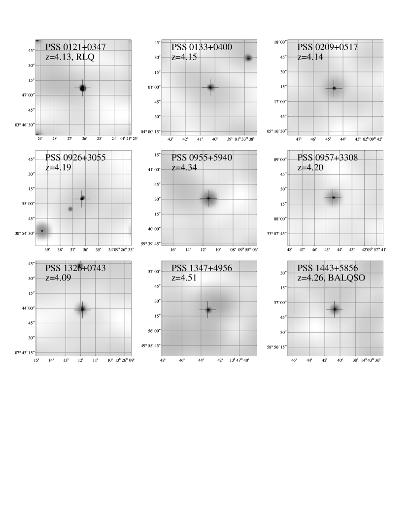
Figure 2: Chandra soft-band (0.5–2 keV) images of the nine high-redshift PSS quasars presented in this paper. In each panel, the horizontal axis shows the Right Ascension, and the vertical axis shows the Declination (both in J2000 coordinates). Each image is 97^′′$\times$ 97^′′. The images have been adaptively smoothed at the 2$\sigma$ level using the algorithm of Ebeling et al. (2002). Crosses mark the optical positions of the quasars. The possible extension of PSS 0926$+$3055 is discussed in $\S$3.5.

2.2 Hobby-Eberly Telescope observations

Optical spectroscopic and photometric observations of all nine quasars have been carried out with the 9-m Hobby-Eberly Telescope (Ramsey et al. 1998). The data were obtained with the HET’s Marcario Low-Resolution Spectrograph (LRS; Hill et al. 1998a,b; Cobos Duenas et al. 1998) within at most $\approx$ 22 days (in the rest frame) of the Chandra observations (see Table 1). High-redshift, high-luminosity quasars ($2<z<3.4$) have longer rest-frame optical variability time scales than low-redshift, low-luminosity quasars ($z<0.4$), and their variations over $\approx$ 1.5 years (in the rest frame) amount to $\approx$ 10% (Kaspi 2001). Therefore, we do not expect our targets to have varied significantly (in the optical) during the time between the optical and X-ray observations. The spectroscopic observations were taken with the 300 line mm^-1 grating, an OG515 blocking filter, and a slit width of 2–3^′′ (depending on the seeing conditions), providing spectra from 5100–10200 Å at a resolving power of $\approx$ 240–300. The exposure time was chosen to be 900 s for all but one of quasars, the exception being for PSS 0957$+$3308 (two close observations of 800 and 900 s, respectively). The spectroscopic data were reduced using standard IRAF routines. Bias exposures taken on each night were stacked and subtracted, and bias-subtracted frames were then flat fielded in a standard manner using internal lamp flats obtained during the same night. The wavelength calibration was performed using a Ne arc lamp, while the flux calibration was achieved using one standard star for each night. The calibrated spectra are shown in Fig. 3.

Figure 3: Optical spectra of the nine PSS quasars presented in this paper obtained with the Hobby-Eberly Telescope at a resolving power of $\approx$ 240–300. The principal emission lines are indicated. Some of them are not reported in Table 4 because of the uncertainties in their measurements. The arrows in the panel for PSS 1443$+$5856 mark the Si IV and C IV broad absorption lines.

Given that there are flux losses due to the slit size and that we did not demand photometric conditions for our optical observations, there is considerable uncertainty in the flux density normalization.

To address the long-term optical variability of the present sample of quasars, we also obtained 120 s $R$-band exposures immediately before the spectroscopic observations. Each image covered a field $\approx 4\hbox{${}^{\prime}$}$ on a side, and using United State Naval Observatory (USNO) photometry of DPOSS objects it was possible to obtain an approximate photometric calibration. Two objects (PSS 0926$+$3055 and PSS 0955$+$5940) showed significant variations (see $\S$4).

3 X-ray analysis

The principal X-ray, optical, and radio properties of our targets are given in Table 3. A description is as follows:
Column (1). — The name of the source.
Column (2). — The Galactic column density (from Dickey & Lockman 1990) in units of 10²⁰ cm^-2.
Column (3). — The monochromatic rest-frame $AB_{1450(1+z)}$ magnitude (defined in $\S$3b of Schneider et al. 1989) with estimated errors $\lower 2.15277pt\hbox{$\;\buildrel<\over{\sim}\;$}0.1$ mag, corrected for Galactic reddening. $AB_{1450(1+z)}$ magnitudes have been derived from HET $R$-band magnitudes assuming the empirical relationship $AB_{1450(1+z)}$=$R-$0.684 $z+3.10$ (effective in the redshift range covered by our sample); see Table 2 of Kaspi et al. (2000). $AB_{1450(1+z)}$ magnitudes have not been derived directly from the spectra because of flux-calibration uncertainties.
Columns (4) and (5). — The 2500 Å rest-frame flux density and luminosity. These were computed from the $AB_{1450(1+z)}$ magnitude assuming an optical power-law slope of $\alpha$=$-$0.79 ($S_{\nu}$ $\propto$ $\nu^{\alpha}$; Fan et al. 2001) to keep consistency with V01; see V01 for further details about the choice of the optical slope. Changing the power-law slope of the optical continuum from $\alpha$=$-$0.79 (Fan et al. 2001) to $\alpha$=$-$0.5 (e.g., Vanden Berk et al. 2001) reduces the 2500 Å rest-frame flux densities and luminosities by $\approx$ 15%.
Column (6). — The absolute $B$-band magnitude calculated according to the formula

$$M_{\rm B}=AB_{1450(1+z)}-5\log D_{\rm L}+5+2.5\log(1+z)-0.83$$ (1)

where $D_{\rm L}$ is the luminosity distance. We note that changing the power-law slope of the optical continuum from $\alpha$=$-$0.79 to $\alpha$=$-$0.5 gives fainter absolute $B$-band magnitudes by $\approx$ 0.35 magnitudes.
Columns (7) and (8). — The observed count rate in the 0.5–2 keV band and the corresponding flux (corrected for Galactic absorption). The 0.5–2 keV counts have been converted into fluxes (using PIMMS Version 3.2d; Mukai 2002) assuming a power-law model with $\Gamma=2$ (as derived for samples of lower redshift quasars; e.g., George et al. 2000; Mineo et al. 2000; Reeves & Turner 2000). Changes of the photon index in the range $\Gamma=$1.7–2.3 lead to only a few percent change in the measured X-ray flux. The soft X-ray flux derived from the 0.5–2 keV counts has also been compared with that derived using the full-band (0.5–8 keV) counts. This comparison gave similar results to within typically 10–20%.
Columns (9) and (10). — The rest-frame 2 keV flux density and luminosity. These were computed assuming the same power-law photon index as in the count-rate-to-flux conversion.
Column (11). — The 2–10 keV rest-frame luminosity corrected for Galactic absorption.
Column (12). — The optical-to-X-ray power-law slope, $\alpha_{\rm ox}$, defined as

$$\alpha_{\rm ox}=\frac{\log(f_{\rm 2~{}keV}/f_{2500~{}\mbox{\scriptsize\AA}})}{\log(\nu_{\rm 2~{}keV}/\nu_{2500~{}\mbox{\scriptsize\AA}})}$$ (2)

where $f_{\rm 2~{}keV}$ and $f_{2500~{}\mbox{\scriptsize\AA}}$ are the flux densities at 2 keV and 2500 Å, respectively. The reported errors have been computed at the $\approx 1\sigma$ level following the “numerical method” described in $\S$ 1.7.3 of Lyons (1991). Both the statistical uncertainties on the X-ray count rates and the effects of possible changes in the X-ray ($\Gamma\approx$ 1.7–2.3) and optical ($\alpha$$\approx$ $-$0.5 to $-$0.9; e.g., Vanden Berk et al. 2001; Schneider et al. 2001) continuum shapes have been taken into account (see $\S$3 of V01 for further details). We note that changing the power-law slope of the optical continuum from $\alpha$=$-$0.79 to $\alpha$=$-$0.5 induces a small increase ($\approx$ 0.03) in the $\alpha_{\rm ox}$ values.
Column (13). — The radio-loudness parameter (e.g., Kellermann et al. 1989), defined as $R$=$f_{\rm 5~{}GHz}/f_{\rm 4400~{}\mbox{\scriptsize\AA}}$ (rest frame). The rest-frame 5 GHz flux density was computed from the FIRST (Becker, White, & Helfand 1995) or NVSS (Condon et al. 1998) observed-frame 1.4 GHz flux density assuming a radio power-law slope of $\alpha=-0.8$. The upper limits reported in the table are at the 3$\sigma$ level. The rest-frame $f_{\rm 4400~{}\mbox{\scriptsize\AA}}$ flux density has been computed from the $AB_{1450(1+z)}$ magnitude assuming an optical power-law slope of $\alpha=-0.79$. Radio-loud quasars (RLQs) are characterized by $R>100$, whereas radio-quiet quasars (RQQs) have $R<10$ (e.g., Kellermann et al. 1989). PSS 0121$+$0347 is radio loud and shows the flattest $\alpha_{\rm ox}$ value in our sample, consistent with results from previous studies (e.g., Zamorani et al. 1981); the other eight objects are radio quiet.

3.1 X-ray flux versus $AB_{1450(1+z)}$ magnitude

Chandra and other exploratory X-ray observations have defined the typical fluxes and luminosities of $z>4$ quasars (e.g., Kaspi et al. 2000; V01; Brandt et al. 2002a, 2002b; Bechtold et al. 2002). Figure 4 shows the observed-frame, Galactic absorption-corrected 0.5–2 keV flux versus $AB_{1450(1+z)}$ magnitude for a compilation of $z\geq 4$ Active Galactic Nuclei (AGNs). The objects presented in this paper are shown as filled triangles, while open triangles and large downward-pointing arrows are previous Chandra observations of high-redshift quasars (e.g., V01; Brandt et al. 2002a), mostly taken from the SDSS. Circled triangles are RLQs, according to the definition in $\S 3$. In the following analyses and plots we exclude all but one (SDSS 120441.73$-$002149.6) of Bechtold Cycle 2 $z>4$ quasars (Bechtold et al. 2002) since they were measured in a different way than all other objects presented here. The ROSAT-detected RQQs and RLQ are plotted as filled circles and a circled star, respectively (Kaspi et al. 2000; V01), while small downward-pointing arrows indicate ROSAT upper limits, most of which are presented here for the first time (see Appendix A for further information). Blazars from the Kaspi et al. (2000) sample are plotted as open stars. One object (the $z=4.01$ blazar GB 1713$+$2148; Hook & McMahon 1998) has its X-ray data published here for the first time and is a $\approx$ 3$\sigma$ ROSAT HRI detection. As a comparison sample, in Fig. 4 we also plot as open circles the $z=4.45$ X-ray selected RQQ RX J1052$+$5719 (Schneider et al. 1998), the $z=5.74$ Broad Absorption Line (BAL) quasar SDSS 1044$-$0125 (Fan et al.

Table 3: Properties of $z>4$ Quasars Observed by Chandra

Object	$N_{\rm H}$	$AB_{1450(1+z)}$	$f_{2500}$	$\log(\nu L_{\nu})_{2500}$	$M_{B}$	Count rate	$f_{\rm x}$	$f_{\rm 2\/keV}$	$\log(\nu L_{\nu})_{\rm 2\/keV}$	$\log(L_{\rm 2-10~{}keV})$	$\alpha_{\rm ox}$	$R$
(1)	(2)	(3)	(4)	(5)	(6)	(7)	(8)	(9)	(10)	(11)	(12)	(13)
PSS 0121$+$0347	3.27	18.5	02.22	46.9	$-$28.4	10.30${}^{+1.60}_{-1.30}$	34.7${}^{+5.4}_{-4.4}$	26.4	45.6	45.8	$-$1.51$\pm{0.06}$	300.2
PSS 0133$+$0400	3.06	18.2	02.93	47.1	$-$28.7	05.25${}^{+1.10}_{-0.92}$	17.4${}^{+3.7}_{-3.0}$	13.4	45.3	45.5	$-$1.67$\pm{0.06}$	$<4.4$
PSS 0209$+$0517	4.73	17.8	04.24	47.2	$-$29.1	03.64${}^{+0.98}_{-0.78}$	12.8${}^{+3.4}_{-2.8}$	09.8	45.2	45.4	$-$1.78${}^{+0.07}_{-0.06}$	$<3.0$
PSS 0926$+$3055	1.88	16.7	11.70	47.7	$-$30.2	08.67${}^{+1.47}_{-1.28}$	27.7${}^{+4.7}_{-4.1}$	21.4	45.5	45.7	$-$1.82$\pm{0.06}$	$<0.3$
PSS 0955$+$5940	1.28	18.4	02.44	47.0	$-$28.6	01.58${}^{+0.72}_{-0.51}$	05.0${}^{+2.2}_{-1.6}$	03.9	44.8	45.0	$-$1.84$\pm{0.08}$	$<5.4$
PSS 0957$+$3308	1.52	18.2	02.93	47.1	$-$28.7	02.98${}^{+0.88}_{-0.69}$	09.4${}^{+2.8}_{-2.2}$	07.3	45.1	45.3	$-$1.77$\pm{0.07}$	$<1.1$
PSS 1326$+$0743	2.01	17.2	07.36	47.4	$-$29.7	07.62${}^{+1.33}_{-1.13}$	24.4${}^{+4.3}_{-3.6}$	18.6	45.4	45.7	$-$1.77$\pm{0.06}$	$<0.5$
PSS 1347$+$4956	1.23	17.4	06.12	47.4	$-$29.7	04.59${}^{+1.07}_{-0.89}$	14.3${}^{+3.4}_{-2.7}$	11.8	45.3	45.5	$-$1.81${}^{+0.07}_{-0.06}$	000.1
PSS 1443$+$5856	1.50	17.7	04.64	47.3	$-$29.3	01.21${}^{+0.83}_{-0.45}$	03.8${}^{+2.6}_{-1.4}$	03.0	44.7	44.9	$-$1.99${}^{+0.10}_{-0.09}$	$<2.8$

Note. — Luminosities are computed using $H_{0}$=70 km s^-1 Mpc^-1, $\Omega_{\rm M}$=0.3, and $\Omega_{\Lambda}$=0.7.

2

2000; Brandt et al. 2001b), and the $z=4.42$ Seyfert galaxy VLA J1236$+$6213 (Waddington et al. 1999; Brandt et al. 2001c). The three filled squares show two quasars and a Seyfert galaxy serendipitously discovered by Chandra (Silverman et al. 2002; Barger et al. 2002) at $z=4.93$, $z=5.18$, and $z=4.13$. The slanted lines show $\alpha_{\rm ox}$ spectral indices of $-$1.5 and $-$1.8 at $z=4.2$, which is the average redshift for the sample discussed in this paper.

Observed-frame, Galactic absorption-corrected 0.5–2 keV flux versus $AB_{1450(1+z)}$ magnitude for $z\geq 4$ AGNs. The objects presented in this paper are plotted as filled triangles, while the open triangles and large downward-pointing arrows indicate previous Chandra observations of high-redshift quasars (V01; Brandt et al. 2002a). Circled triangles are RLQs. The ROSAT-detected RQQs and RLQ are plotted as filled circles and a circled star, respectively (Kaspi et al. 2000; V01), while small downward-pointing arrows indicate ROSAT upper limits (most of the upper limits are presented here for the first time; see Appendix A for details). Blazars from the Kaspi et al. (2000) sample are plotted as open stars (one object is published here for the first time; see Appendix A). For comparison, we have plotted as open circles the $z=4.45$ X-ray selected RQQ RX J1052$+$5719 (Schneider et al. 1998), the $z=5.74$ RQQ SDSS J1044$-$0125 (Fan et al. 2000; Brandt et al. 2001b), and the $z=4.42$ Seyfert galaxy VLA J1236$+$6213 (Waddington et al. 1999; Brandt et al. 2001c). The three filled squares indicate $z>4$ AGNs serendipitously discovered by Chandra (Silverman et al. 2002; Barger et al. 2002). The slanted lines show $\alpha_{\rm ox}$=$-$1.5 and $\alpha_{\rm ox}$=$-$1.8 loci at $z=4.2$ (the average redshift of the present sample), assuming the same X-ray and optical spectral shapes used in the text.

As shown in Fig. 4, quasars at $z>4$ are generally faint X-ray sources, with 0.5–2 keV fluxes $<4\times~{}10^{-14}$ ${\rm erg~{}cm}^{-2}~{}{\rm s}^{-1}$ . The PSS quasars presented in this paper are among the X-ray brightest known and allow study of a region of the luminosity-redshift parameter space different from that of most of the SDSS quasars observed in X-rays to date (e.g., V01; Brandt et al. 2002a), which are usually optically less luminous and located at higher redshift. Given the X-ray fluxes found from Chandra snapshot observations, it is clear that PSS and BRI quasars represent the best known RQQs at $z>4$ for longer XMM-Newton spectroscopic observations. Individual XMM-Newton spectra, coupled with stacked Chandra spectra, can provide tighter spectral constraints and possibly allow searches for spectral features such as iron K$\alpha$ lines.

In Fig. 4 there is a correlation between the soft X-ray flux (corrected for Galactic absorption) and $AB_{1450(1+z)}$ magnitude. Given the presence of upper limits, to study this correlation we have used the ASURV software package Rev 1.2 (LaValley, Isobe, & Feigelson 1992). To evaluate the significance of this correlation, we used several methods available in ASURV, namely the Cox regression proportional hazard (Cox 1972), the generalized Kendall’s $\tau$ (Brown, Hollander, & Korwar 1974), and the Spearman’s $\rho$ models. Using the Chandra RQQs, the correlation is significant at the 99.5–99.8% and 99.99% levels when all the PSS/BRI and PSS/BRI/SDSS quasars are taken into account, respectively. In the latter case, the best-fit relationship is parameterized by $f_{\rm X}=[-(6.9\pm{1.0})\ AB_{1450(1+z)}+(137\pm{19})]\times 10^{-15}$ ${\rm erg~{}cm}^{-2}~{}{\rm s}^{-1}$ . Note that the scatter around the best-fit relationship is significant (a factor of $\approx$ 3). The BALQSOs have been excluded in these correlation analyses because they are known to be significantly absorbed in the X-ray band (e.g., Brandt, Laor, & Wills 2000; Gallagher et al. 2001, 2002; Green et al. 2001; see also V01 for discussion about the BALQSOs previously observed and undetected by Chandra at $z>4$). Including also the RQQs with ROSAT detections or tight upper limits (i.e., $\alpha_{\rm ox}$$<-1.5$) provides a significance $>99.99$% for the above correlation. The observed correlation indicates that the optical and X-ray emission are likely to be powered by the same engine, namely accretion onto a supermassive black hole. The large 2–10 keV rest-frame luminosities of the PSS objects investigated in this paper ($\approx$ $10^{44.9-45.8}$ erg s^-1) suggest that the X-ray emission is mostly nuclear and not related to the starburst component whose existence has been suggested by recent observations at millimeter and sub-millimeter wavelengths (e.g., Omont et al. 2001; Isaak et al. 2002; see also Elvis, Marengo, & Karovska 2002 for a different interpretation).

3.2 $\alpha_{\rm ox}$ results

The average $\alpha_{\rm ox}$ for the eight RQQs of the present PSS sample is $\langle\alpha_{\rm ox}\rangle$=$-$1.81$\pm{0.03}$ (the quoted errors represent the standard deviation of the mean), with the BALQSO PSS 1443$+$5856 (see $\S$4) being the quasar with the steepest $\alpha_{\rm ox}$ in our sample ($\alpha_{\rm ox}$=$-1.99^{+0.10}_{-0.09}$). Even after removing the BALQSO, the average $\alpha_{\rm ox}$ is $-$1.78$\pm{0.02}$, still considerably steeper than that obtained for samples of lower-luminosity, local quasars [e.g., the Bright Quasar Survey (BQS; Schmidt & Green 1983) quasars at $z<0.5$ have $\langle\alpha_{\rm ox}\rangle$=$-$1.56$\pm{0.02}$; see Brandt et al. 2000 and V01]. The same applies when all the PSS/BRI ($\langle\alpha_{\rm ox}\rangle$=$-$1.78$\pm{0.03}$) or the SDSS ($\langle\alpha_{\rm ox}\rangle$=$-$1.75$\pm{0.03}$) $z>4$ quasars observed by Chandra are taken into account. These average $\alpha_{\rm ox}$ values are slightly flatter (typically by 0.02–0.03) when the BALQSOs are excluded from the analysis. One possible explanation for the more negative $\alpha_{\rm ox}$ values seen at $z>4$ is the presence of X-ray absorption; however, we find no evidence of X-ray absorption either from the individual quasars’ spectra (see Table 2) or from the joint spectral fitting discussed in $\S$3.3. Another possibility is that $\alpha_{\rm ox}$ depends upon 2500 Å rest-frame luminosity (e.g., Avni, Worrall, & Morgan 1995) or redshift (e.g., Bechtold et al. 2002). We have searched for significant correlations of $\alpha_{\rm ox}$ with either 2500 Å rest-frame luminosity (Fig. 5a) or redshift (Fig. 5b)  at

(a) $\alpha_{\rm ox}$ versus $\log\ L_{2500~{}\rm\AA}$ and (b) redshift for $z\geq 4$ optically selected RQQs. Symbols are the same as in Fig. 4.

$z>4$ using the statistical methods available in ASURV (see $\S$3.1) but found none. Given the small spread in UV luminosities and redshifts of the objects used in this analysis, we cannot address the question of $\alpha_{\rm ox}$ changes with rest-frame 2500 Å luminosity or redshift effectively. However, the analysis of SDSS quasars in the redshift range $z\approx$ 0.2–6.3 using partial correlation analysis (Vignali, Brandt, & Schneider 2002) shows that $\alpha_{\rm ox}$ is mainly dependent upon 2500 Å luminosity.

3.3 Joint spectral fit

To provide tighter constraints on the average X-ray spectral properties of $z>4$ quasars, we have performed a joint spectral analysis of our target quasars. Source counts have been extracted from 2^′′ radius circular apertures centered on the X-ray position of each quasar. The background has been taken from annuli centered on the sources, avoiding the presence of nearby faint X-ray sources. To account for the recently discovered quantum efficiency decay of ACIS at low energies, possibly caused by molecular contamination of the ACIS filters, we have applied a time-dependent correction to the ACIS quantum efficiency generating a new ancillary response file (ARF) for each source. The quantum efficiency degradation is not severe at energies above $\approx$ 0.7 keV ($\approx$ 10% at 1 keV), where most of the detected signal lies, but, if left uncorrected, it might affect the results at lower energies. In particular, the reduction in efficiency could produce unreliable column densities if not taken into account properly.

Only two objects are characterized by low counting statistics ($\approx$ 10 counts); all the others have $\approx$ 20–70 counts in the 0.5–8 keV band. The sample does not seem to be biased by the presence of either a few high signal-to-noise ratio objects (see Table 2) or the RLQ PSS 0121$+$0347, whose X-ray photon index (derived from the band ratio analysis; see Table 2) is consistent with those of the other quasars. Spectral analysis was carried out with XSPEC. The joint spectral fitting of the nine individual unbinned quasar spectra was carried out using the Cash statistic (Cash 1979). The Cash statistic is particularly well suited to low-count sources (e.g., Nousek & Shue 1989), and, since it is applied to the unbinned data, it allows us to retain all the spectral information. Furthermore, we can apply to each source its own Galactic absorption and redshift. The resulting joint spectrum, although derived from only $\approx$ 340 counts, is reasonably good due to the extremely low background of Chandra (there are only $\approx$ 2.1 background counts in all source cells), and it allows spectral analysis in the $\approx$ 2–30 keV rest-frame band. Joint fitting with a power-law model (leaving the normalizations free to vary) and Galactic absorption provides a good fit (as judged by the small data-to-model residuals and checked with 10000 Monte-Carlo simulations) with a photon index of $\Gamma$=1.98$\pm{0.16}$ (errors are at the 90% confidence level; $\Delta\chi^{2}$=2.71, Avni 1976). This photon index is consistent with those obtained for lower-redshift samples of RQQs in the 2–10 keV band (e.g., George et al. 2000; Mineo et al. 2000; Reeves & Turner 2000) and with that of the BALQSO APM 08279$+$5255 at $z=3.91$ (Chartas et al. 2002; $\Gamma$=1.72${}^{+0.06}_{-0.05}$). The photon index is also consistent with the average $\Gamma$ determined from the band ratios (see Table 2) using ASURV ($\langle\Gamma\rangle$=2.07$\pm{0.13}$). The combined spectrum (used here only for presentation purposes), fitted with the power-law model described above, is shown in Fig. 6. Bechtold et al. (2002) reported an X-ray spectral flattening with redshift for quasars, with photon indices in the range $\Gamma\approx$ 1.2–1.6 ($\langle\Gamma\rangle$=1.48$\pm{0.13}$) at $z\approx$ 3.7–6.3. The present data, obtained for an optically brighter sample of quasars, are not consistent with such claims.

Combined quasar spectrum (used only for presentation purposes) fitted with the best-fit power-law model and Galactic absorption (see $\S$3.3 for details). The 68, 90, and 99% confidence regions for the photon index and intrinsic column density obtained using the Cash statistic are shown in the insert. Data-to-model residuals are shown in the bottom panel (in units of $\sigma$).

Furthermore, we have constrained the presence of neutral intrinsic absorption. In the absorption column we have assumed solar abundances, although there are indications of supersolar abundances of heavy elements in high-redshift quasar nuclei (e.g., Hamann & Ferland 1999; Constantin et al. 2002). Doubling the abundances in the fit gives a reduction in the column density of a factor of $\approx$ 2. There is no evidence for absorption in excess of the Galactic column density, as shown in the insert in Fig. 6, where the 68, 90, and 99% confidence regions for the photon index and intrinsic column density are plotted. Although it is not possible to rule out substantial X-ray absorption in the individual spectrum of any one quasar, on average it appears that any neutral absorption has a column density of $N_{\rm H}\lower 2.15277pt\hbox{$\;\buildrel<\over{\sim}\;$}8.8\times 10^{21}$ cm^-2 (at 90% confidence). Note that this average constraint is more generally applicable than if we had just a $\approx$ 340-count spectrum of a single $z>4$ quasar, since any one quasar might always be exceptional. If our targets had intrinsic absorption of $N_{\rm H}\approx$ (2–5)$\times 10^{22}$ cm^-2, as recently found in two RQQs at $z\approx$ 2 using ASCA data (Reeves & Turner 2000), we would be able to detect it given the upper limit on the column density we derived. We have also investigated the possible presence of ionized absorption using the model ABSORI in XSPEC. While, of course, this is more difficult to constrain in general, our data do not provide any suggestion of ionized absorption. Furthermore, considering narrow iron K$\alpha$ lines in the rest-frame energy range 6.4–6.97 keV, the typical upper limit on the equivalent width (EW) is $\approx$ 420 eV.

3.4 Companion objects

Schwartz (2002b) tentatively associated an X-ray source 23^′′ from the $z=5.99$ quasar SDSS 1306$+$0356 with an X-ray jet, although neither the source nor SDSS 1306$+$0356 have any radio emission in the FIRST catalog (Becker et al. 1995). To date, no quasar with X-ray emission undoubtedly associated with jets is radio quiet, all being powerful radio sources (e.g., Harris & Krawczynski 2002). Moreover, the jets are characterized by substantial radio emission (e.g., Siemiginowska et al. 2002; Brunetti et al. 2002 and references therein) even after correction for boosting. If the X-ray emission from jets is produced via the Compton scattering of cosmic microwave background (CMB) photons by relativistic electrons, then the enhancement of the CMB energy density with redshift compensates for the decrease of surface brightness (see Schwartz 2002a for details; also see Rees & Setti 1968). Recently, Ivanov (2002) detected the $I$-band counterpart of the X-ray source 23^′′ from SDSS 1306$+$0356. The elongation of the $I$-band counterpart suggests the presence of a foreground galaxy, rather than UV/optical emission from a jet associated with SDSS 1306$+$0356, but no redshift for the counterpart has yet been measured.

In the present sample of nine objects, only one quasar, PSS 0121$+$0347, is radio loud (see $\S$3). Nevertheless, we have searched for possible companions/jets for all the objects in our sample over a region of $\approx$ 100^′′$\times$100^′′ centered on the quasars (the same shown in the images of Fig. 2). At $z\approx$ 4–4.5, this corresponds to a linear scale of $\approx$ 320 kpc at each side of the quasar. We found some faint objects (about one per field); none of these is X-ray bright and close enough to our targets to contaminate their X-ray emission. Most of the serendipitous X-ray sources lack counterparts in the DPOSS images, and none of them has associated radio emission down to a 1.4 GHz flux density of $\approx$ 0.5–1.5 mJy (3$\sigma$).

As an observational check, we compared the 0.5–2 keV cumulative number counts of sources detected in the current high-redshift quasar fields with the number counts obtained from the Chandra Deep Field-North survey (Brandt et al. 2001a) and the ROSAT deep survey of the Lockman Hole (Hasinger et al. 1998); the high-redshift quasars themselves, of course, were excluded. The surface density of X-ray sources surrounding the PSS quasars at the flux limit we reached ($\approx 10^{-15}$ ${\rm erg~{}cm}^{-2}~{}{\rm s}^{-1}$ ) is $N(>S$)=1224${}^{+612}_{-429}$ deg^-2, consistent with the densities obtained in deep-field observations. Thus we find no evidence for an excess of companions/jets associated with our quasars.

3.5 X-ray extension of the quasars

To constrain the presence of either gravitational lensing (e.g., Barkana & Loeb 2000; Wyithe & Loeb 2002; Comerford, Haiman, & Schaye 2002) or X-ray jets close to the sources (e.g., Schwartz 2002b), we performed an analysis of X-ray extension for all the quasars in the present sample. At $z\approx$ 4–5, the angular separation between the images of a multiply imaged source should often be $\approx$ 1–2^′′, depending on the adopted dark matter model (Barkana & Loeb 2000), and Chandra has been able to detect and separate lensed images up to $z\approx$ 3.9 (Chartas et al. 2002). For each quasar, we created a point spread function (PSF) at $\approx$ 1.5 keV at the source position (using the tool MKPSF) normalized by the effective number of source counts. Then we compared the radial profile of this PSF with that of the source, finding good agreement in the radial counts distribution. For one quasar (PSS 0926$+$3055) we performed a further check given the presence in the soft band of three counts “pointing” in the North-West direction within a radius of 3^′′ of the source, although there is no indication of extension in the optical image. We deconvolved the X-ray source image with the PSF and found that the counts distribution still seems to be in agreement with the source being point-like. However, further investigation with a longer Chandra observation is needed to completely rule out the possibility of PSS 0926$+$3055 being slightly extended.

3.6 X-ray variability of the quasars

Although the present observations are short (the observation length in the rest frame is $\approx$ 15 minutes), we searched for X-ray variability of our targets. There are tentative reports that quasar X-ray variability increases with redshift (e.g., Manners, Almaini, & Lawrence 2002). We analyzed the photon arrival times in the 0.5–8 keV band using the Kolmogorov-Smirnov (KS) test. No significant variability was detected (the KS probabilities that the sources are variable range from $\approx$ 6% to 83%). Our constraints on the amplitude of variability depend upon the number of counts detected as well as the putative variability timescale. Systematic variability sustained over a period of $\approx$ 5–6 ks (in the observed frame) must be less than $\approx$ 30–90%.

4 Optical analysis

Following the method described in $\S$2.2, two quasars, PSS 0926$+$3055 and PSS 0955$+$5940, have been found to vary in the optical band on a timescale of $\approx$ 6 years (in the observed

Table 4: Emission-Line Measurements

	Ly$\alpha$ (1216 Å)			N V (1240 Å)				O I (1304 Å)					Si IV-O IV] (1394-1402 Å)					C IV (1549 Å)
Object Name	$\lambda$	EW		$\lambda$	EW	$z$		$\lambda$	EW	FWHM	$z$		$\lambda$	EW	FWHM	$z$		$\lambda$	EW	FWHM	$z$	$\langle z\rangle$
PSS 0121$+$0347	6232.3	81.1		$\cdots$	$\cdots$	$\cdots$		6674.4	4.8	1020	4.112		$\cdots$	$\cdots$	$\cdots$	$\cdots$		7963.6	33.5	3810	4.142	4.126
PSS 0133$+$0400	6266.1	25.9		6391.7	2.3	4.152		6734.8	10.3	6270	4.158		7218.4	5.3	2550	4.150		7999.7	32.6	7370	4.165	4.155
PSS 0209$+$0517	6326.1	33.5		$\cdots$	$\cdots$	$\cdots$		$\cdots$	$\cdots$	$\cdots$	$\cdots$		7216.8	1.1	3350	4.149		7945.1	12.0	12940	4.130	4.143
PSS 0926$+$3055	6309.0	44.0		$\cdots$	$\cdots$	$\cdots$		6802.6	1.3	1460	4.210		7261.6	8.2	6620	4.181		8028.1	18.5	5880	4.184	4.191
PSS 0955$+$5940	6503.5	285.0		$\cdots$	$\cdots$	$\cdots$		6979.2	3.9	2270	4.345		7471.1	4.0	2730	4.330		8270.0	21.6	4220	4.340	4.339
PSS 0957$+$3308	6386.9	22.1		$\cdots$	$\cdots$	$\cdots$		6829.5	1.2	2150	4.231		7267.2	9.4	6340	4.185		8020.7	12.1	9500	4.179	4.198
PSS 1326$+$0743	6223.6	26.2		6306.3	4.2	4.083		6670.6	1.6	2260	4.109		7122.7	10.0	7130	4.082		7905.4	21.2	10920	4.105	4.089
PSS 1347$+$4956	6760.6	8.7		$\cdots$	$\cdots$	$\cdots$		$\cdots$	$\cdots$	$\cdots$	$\cdots$		7708.4	4.1	5630	4.500		8535.3	15.9	7670	4.511	4.506
PSS 1443$+$5856	6465.0	69.5		$\cdots$	$\cdots$	$\cdots$		$\cdots$	$\cdots$	$\cdots$	$\cdots$		7369.2	9.9	6760	4.258		8161.8	19.0	7980	4.270	4.264

Note. — The redshift for each quasar was determined by averaging the emission lines (excluding Ly$\alpha$ for all objects). The last column reports the weighted average for the redshift. The FWHMs of Ly$\alpha$ and N V are not reported because of the uncertainties in their measurements (see, e.g., Schneider et al. 1991).

2

frame). The HET $R$-band magnitude for the former is 0.3 mag brighter than the value reported in the Djorgovski list (taking into account the different filter transmission and bandpass; see Footnote 4), while the latter appears 0.5 mag fainter. These are the only objects for which significant long-term optical variability has been found.

The principal emission-line measurements are presented in Table 4. The centroids of the emission lines were determined with Gaussian fits. Redshifts have been derived from HET spectra averaging the emission-line redshifts (excluding Ly$\alpha$, whose measurements are affected by many uncertainties; see, e.g., Schneider, Schmidt, & Gunn 1991). Typical uncertainties are $\approx$ 0.01 for non-BALQSO redshift measurements, and $\approx$ 10–15% and $\approx$ 5–10% for FWHM and EW measurements, respectively. We have compared the C IV emission-line equivalent widths of our objects with those derived for the Constantin et al. (2002) sample of optically luminous $z>4$ PSS and BRI quasars; we found good agreement. One of our quasars, PSS 1443$+$5856, shows broad C IV and Si IV absorption features in its optical spectrum (see Fig. 3) with a blueshift of $\approx$ 10000 km s^-1 with respect to the systemic redshift of the quasar. The C IV absorption-line EW is $\approx$ 14 Å (rest frame), which is close to the value expected from the $\alpha_{\rm ox}$–C IV EW anti-correlation found for low-redshift quasars (see Fig. 4 of Brandt et al. 2000). The likely existence of this anti-correlation at $z>4$ has already been verified (e.g., Maiolino et al. 2001; Goodrich et al. 2001; also see V01). Given the correlation between $AB_{1450(1+z)}$ and soft X-ray flux shown in Fig. 4, the X-ray detection of PSS 1443$+$5856 is not surprising. Since this quasar is 1.5–1.7 magnitudes brighter than the previously X-ray undetected $z>4$ BALQSOs (V01), a higher X-ray flux is expected.

5 Summary and implications

We have presented the Chandra X-ray detections of nine high-redshift ($z\approx$ 4.1–4.5) quasars. These quasars were targeted because they are among the most optically luminous objects in the Universe and are likely to comprise a significant fraction of the most luminous $z>4$ optically selected objects. Their SEDs are characterized by steeper (more negative) optical-to-X-ray spectral indices ($\langle\alpha_{\rm ox}\rangle$=$-$1.81$\pm{0.03}$) compared to samples of optically selected quasars at low or intermediate redshift. Given their large mean 2500 Å luminosity density ($\approx$ 1.6$\times 10^{32}$ erg s^-1 Hz^-1), their steep $\alpha_{\rm ox}$ values may be explained in the context of the $\alpha_{\rm ox}$–ultraviolet luminosity anti-correlation found in other work (e.g., Avni et al. 1995; Vignali et al. 2002). We also confirm the presence of a significant correlation between the optical magnitude and soft X-ray flux previously found by V01 for a more heterogeneous sample of $z>4$ quasars. Joint spectral fitting in the $\approx$ 2–30 keV rest-frame band indicates that optically selected, luminous $z>4$ quasars are characterized, on average, by a power-law model with a photon index of $\approx$ 2.0$\pm{0.2}$, similar to the majority of lower-redshift quasars. There is no evidence for intrinsic absorption ($N_{\rm H}\lower 2.15277pt\hbox{$\;\buildrel<\over{\sim}\;$}8.8\times 10^{21}$ cm^-2 at the 90% confidence level).

We also have presented near-simultaneous optical spectra obtained with the HET. Optical spectra for seven of these quasars are published here for the first time. One of the quasars, PSS 1443$+$5856, shows broad absorption features in C IV and Si IV.

From a more general perspective, our results show that $z\approx$ 4.1–4.5 quasars and local quasars have reasonably similar X-ray and broad-band spectra (once luminosity effects are taken into account). The small-scale X-ray emission regions of quasars do not appear to be sensitive to the substantial large-scale environmental differences between $z\approx 4$ and $z\approx 0$. The lack of any strong X-ray spectral changes is particularly relevant since X-ray emission originates from the compact region where accretion, and thus black hole growth, occurs. Our data do not provide any hints for different accretion/growth mechanisms (via, e.g., accretion-disk instabilities or “trapping radius” effects) between the most luminous high-redshift quasars and local quasars. Furthermore, our data suggest that (1) minimum black hole masses for high-redshift quasars can be estimated reasonably well via the Eddington limit by adopting the bolometric correction used for comparably luminous low-redshift quasars, and (2) calculations of the effects of early quasars upon the intergalactic medium can, at least to first order, adopt the spectral energy distributions of comparably luminous low-redshift quasars. Finally, our data support the dogma that X-ray emission is a universal property of quasars at all redshifts. Quasars at even higher redshifts ($z\approx$ 5–15) will likely be luminous X-ray sources that can be detected in future X-ray surveys.

(a) Simulated 40 ks spectrum and (b) 68, 90, and 99% confidence regions for the He-like iron K$\alpha$ emission-line energy and intensity using the calorimeter and the grating onboard Constellation-X. We have used the observed Chandra 0.5–2 keV flux of $\approx$ 2.8 $\times\ 10^{-14}$  ${\rm erg~{}cm}^{-2}~{}{\rm s}^{-1}$ and assumed a $\Gamma=2.0$ power-law spectrum with Galactic absorption. We also included a narrow iron K$\alpha$ emission line with a rest-frame equivalent width of 70 eV (see $\S$5 for details). (c) 68, 90, and 99% confidence regions for intrinsic column density and photon index. The “X” marks the input parameters of the simulation, while the “$+$” indicates the best-fit result.

6 Future work

We have recently been awarded 11 additional Chandra observations of $z>4$ optically luminous quasars. These observations will provide tighter constraints on the X-ray properties of high-redshift quasars, thus allowing for more feasible planning of X-ray observations with next-generation, large-area X-ray telescopes. In this regard, we have simulated a 40 ks Constellation-X  spectrum (with the calorimeter and the first-order grating; see Fig. 7a) of the X-ray brightest RQQ of our sample, PSS 0926$+$3055 at $z=4.19$, assuming a power-law spectrum with $\Gamma$=2.0 and Galactic absorption. A narrow ($\sigma$=10 eV), He-like (at 6.7 keV) iron K$\alpha$ emission line with a rest-frame equivalent width of $\approx$ 70 eV has also been included in the model. At high X-ray luminosities ($L_{\rm 2-10~{}keV}$$>$10^44-45 erg s^-1) the iron K$\alpha$ line is expected to be ionized and fairly weak, with most of the line flux coming from its core (the “X-ray Baldwin effect” discussed in Nandra et al. 1997; see also Iwasawa & Taniguchi 1993). The 68, 90, and 99% confidence regions for the line energy and intensity are plotted in Fig. 7b. Constellation-X would gather $\approx$ 11300 counts ($\approx$ 8500 from the calorimeter and $\approx$ 2800 from the first-order grating) in the observed 0.25–10 keV band. These would ensure a good accuracy in the measurements of the X-ray parameters; in particular, the photon index, line energy, and line EW would be measured with accuracies of $\approx$ 1.2%, 0.1%, and 29%, respectively. We are able to detect ionized iron K$\alpha$ lines down to rest-frame EWs of $\approx$50 eV. Due to its low-energy coverage, Constellation-X can also place significant constraints on the intrinsic column density down to $N_{\rm H}\approx 2\times 10^{21}$ cm^-2 (see Fig. 7c).

Appendix A New ROSAT upper limits for $z\geq 4$ quasars and a tentative detection of GB 1713$+$2148

The Djorgovski list of $z\geq 4$ quasars (see Footnote 4) has been cross correlated with ROSAT PSPC and HRI archival observations. In the 0.5–2 keV energy band, we found 45 new upper limits [34 RQQs, five RLQs, four quasars with loose radio loudness upper limits ($R\lower 2.15277pt\hbox{$\;\buildrel<\over{\sim}\;$}15$), and two quasars without FIRST/NVSS coverage] and a tentative $\approx$ 3$\sigma$ detection for the blazar GB 1713$+$2148 (in an HRI observation). The 3$\sigma$ upper limits (reported in Table A1) have been derived in a similar way to those shown in Table 4 of V01 using the SOSTA command in the XIMAGE package (Giommi et al. 1992). For the 3$\sigma$ detection of GB 1713$+$2148, we cross checked the results obtained with the maximum likelihood method available with the MIDAS/EXSAS package (Zimmermann et al. 1998) with the XIMAGE results. GB 1713$+$2148 is unusually X-ray faint compared to the other blazars, despite its large radio flux density ($\approx$ 450 mJy in the NVSS; $R\approx$ 24400).

For SDSS quasars, the $AB_{1450(1+z)}$ magnitudes have been derived from the $i$-band filter using either the empirical relationship $AB_{1450(1+z)}$=$i-0.2$ or the method described in Vignali et al. (2002) for the SDSS quasars in the Early Data Release (Schneider et al. 2002). For the other quasars, the $AB_{1450(1+z)}$ magnitudes have been derived either from the $R$-band magnitude using the empirical relationship $AB_{1450(1+z)}$=$R-$0.684 $z+3.10$ or from the $r$-band magnitude using $AB_{1450(1+z)}$=$r-$0.684 $z+2.75$. Unless otherwise stated, the $R$- and $r$-band magnitudes have been obtained from the Djorgovski list (see Footnote 4). All of the above relationships provide reliable $AB_{1450(1+z)}$ estimates (within $\approx$ 0.1–0.2 magnitudes) in the redshift range under consideration.

Table A1: Properties of $z\geq 4$ Quasars in ROSAT Fields

Object	$z$	$AB_{1450(1+z)}$	$M_{B}$	$f_{\rm x}$	$\alpha_{\rm ox}$
ROSAT RQQs
PSS 0014$+$3032	4.47	18.5	$-$28.6	$<4.44$	$<-1.45$
BRI 0046$-$2458	4.15	18.9	$-$28.1	$<3.97$	$<-1.43$
SDSS 0127$-$0045	4.06	17.9	$-$29.0	$<3.53$	$<-1.60$
PSS 0134$+$3307	4.53	18.5	$-$28.6	$<13.3$	$<-1.27$
PSS 0223$+$2325	4.27	18.8	$-$28.2	$<12.3$	$<-1.25$
SDSS 0239$-$0810	4.00	19.4	$-$27.4	$<1.90$	$<-1.47$
SDSS 0252+0031	4.10	19.7	$-$27.2	$<11.8$	$<-1.13$
BR 0300$-$0207	4.25	18.4	$-$28.6	$<8.46$	$<-1.37$
BR 0353$-$3820	4.55	17.6	$-$29.5	$<11.7$	$<-1.43$
FIRST 0747$+$2739	4.11	18.2	$-$28.7	$<11.3$	$<-1.36$
PSS 0808$+$5215	4.44	18.5	$-$28.5	$<4.58$	$<-1.45$
SDSS 0810$+$4603	4.07	18.2	$-$28.7	$<7.03$	$<-1.55$
SDSS 0832$+$5303	4.02	19.6	$-$27.3	$<22.0$	$<-1.08$
PSS 0852$+$5045	4.20	18.0	$-$29.0	$<7.24$	$<-1.47$
SDSS 0904$+$5350	4.25	19.1	$-$27.9	$<3.90$	$<-1.40$
PSS 1026$+$3828	4.18	18.8	$-$28.1	$<3.20$	$<-1.47$
SDSS 1034$-$0027	4.38	19.8	$-$27.2	$<7.48$	$<-1.17$
SDSS 1040$-$0015	4.32	18.7	$-$28.3	$<8.28$	$<-1.32$
SDSS 1048$-$0028	4.00	19.2	$-$27.7	$<4.66$	$<-1.35$
SDSS 1052$-$0006	4.13	19.6	$-$27.3	$<3.33$	$<-1.34$
SDSS 1056$+$0032	4.02	19.8	$-$27.1	$<9.52$	$<-1.15$
SDSS 1059$+$0104	4.06	19.4	$-$27.6	$<8.61$	$<-1.23$
PSS 1140$+$6205	4.51	18.4	$-$28.7	$<2.86$	$<-1.54$
PSS 1226$+$0950	4.34	18.6	$-$28.4	$<7.04$	$<-1.37$
PSS 1248$+$3110	4.32	19.1	$-$27.9	$<4.60$	$<-1.37$
PSS 1315$+$2924	4.18	18.4	$-$28.6	$<1.66$	$<-1.65$
PSS 1339$+$5154	4.08	19.0	$-$27.9	$<1.21$	$<-1.61$
PSS 1401$+$4111	4.01	18.6	$-$28.2	$<13.2$	$<-1.27$
PSS 1418$+$4449	4.32	18.5	$-$28.5	$<3.69$	$<-1.48$
PSS 1430$+$2828	4.30	19.5	$-$27.5	$<5.38$	$<-1.28$
PSS 1543$+$3417	4.41	18.5	$-$28.5	$<13.7$	$<-1.27$
PSS 1555$+$2003	4.22	19.1	$-$27.8	$<4.26$	$<-1.38$
PSS 1745$+$6846	4.13	19.1	$-$27.9	$<0.87$	$<-1.65$
PSS 2155$+$1358	4.26	18.2	$-$28.8	$<7.73$	$<-1.42$
ROSAT RLQs
SDSS 0300$+$0032	4.19	19.9	$-$27.0	$<5.19$	$<-1.22$
PSS 0439$-$0207	4.40	18.8	$-$28.2	$<5.55$	$<-1.37$
SDSS 0913$+$5919	5.11	20.3	$-$27.0	$<8.70$	$<-1.05$
CLASS 0915$+$068	4.19	18.9	$-$28.0	$<7.08$	$<-1.32$
CLASS 1322$+$116	4.40	18.9	$-$28.1	$<7.47$	$<-1.31$
ROSAT quasars with loose radio loudness upper limits
SDSS 0338$-$RD657	4.96	21.1	$-$26.1	$<8.63$	$<-0.93$
SDSS 0405$+$0059	4.05	19.8	$-$27.1	$<10.0$	$<-1.13$
SDSS 1708$+$6022	4.35	19.8	$-$27.2	$<2.60$	$<-1.34$
SDSS 1710$+$5923	4.47	19.7	$-$27.4	$<6.00$	$<-1.23$
ROSAT quasars without FIRST/NVSS coverage
BR 0413$-$4405	4.07	19.2	$-$27.7	$<25.1$	$<-1.07$
BR 0418$-$5723	4.46	18.8	$-$28.3	$<21.6$	$<-1.15$
ROSAT Blazar
GB 1713$+$2148	4.01	21.4	$-$25.5	2.81	$-$1.11

Note. — The division between RQQs and RLQs is based on the radio-loudness parameter (defined in $\S$3).

References

- (1) Anderson, S. F., et al. 2001, AJ, 122, 503
- (2) Arnaud, K. A. 1996, in ASP Conf. Ser. 101, Astronomical Data Analysis Software and Systems V, ed. G. Jacoby, & J. Barnes (San Francisco: ASP), 17
- (3) Avni, Y. 1976, ApJ, 210, 642
- (4) Avni, Y., Worrall, D. M., & Morgan Jr., W. A. 1995, ApJ, 454, 673
- (5) Barger, A. J., Cowie, L. L., Brandt, W. N., Capak, P., Garmire, G. P., Hornschemeier, A. E., Steffen, A. T., & Wehner, E. H. 2002, AJ, 124, 1839
- (6) Barkana, R., & Loeb, A. 2000, ApJ, 531, 613
- (7) Bechtold, J., et al. 2002, ApJ, in press (astro-ph/0204462)
- (8) Becker, R. H., White, R. L., & Helfand, D. J. 1995, ApJ, 450, 559
- (9) Becker, R. H., et al. 2001, AJ, 122, 2850
- (10) Begelman, M. C. 1978, MNRAS, 184, 53
- (11) Bertin, E., & Arnouts, S. 1996, A&AS, 117, 393
- (12) Brandt, W. N., Laor, A., & Wills, B. J. 2000, ApJ, 528, 637
- (13) Brandt, W. N., et al. 2001a, AJ, 122, 2810
- (14) Brandt, W. N., Guainazzi, M., Kaspi, S., Fan, X., Schneider, D. P., Strauss, M. A., Clavel, J., & Gunn, J. E. 2001b, AJ, 121, 591
- (15) Brandt, W. N., et al. 2001c, AJ, 122, 1
- (16) Brandt, W. N., et al. 2002a, ApJ, 569, L5
- (17) Brandt, W. N., Vignali, C., Fan, X., Kaspi, S., & Schneider, D. P. 2002b, in X-ray Spectroscopy of AGN with Chandra and XMM-Newton, ed. Th. Boller, S. Komossa, S. Kahn, H. Kunieda, & L. Gallo (Garching: MPE Press), 235
- (18) Brown, B. W. M., Hollander, M., & Korwar, R. M. 1974, in Reliability and Biometry, ed. F. Proschan, & R. J. Serfling (Philadelphia: SIAM), 327
- (19) Brunetti, G. 2002, in NATO Conf. Series, The Role of VLBI in Astrophysics, Astronomy and Geodesy, ed. F. Mantovani, & A. J. Kus, in press (astro-ph/0207671)
- (20) Carilli, C. L., Bertoldi, F., Omont, A., Cox, P., McMahon, R. G., & Isaak, K. G. 2001a, AJ, 122, 1679
- (21) Carilli, C. L., et al. 2001b, ApJ, 555, 625
- (22) Cash, W. 1979, ApJ, 228, 939
- (23) Chartas, G., Brandt, W. N., Gallagher, S. C., & Garmire, G. P., 2002, ApJ, in press (astro-ph/0207196)
- (24) Cobos Duenas, F. J., Tejada, C., Hill, G. J., & Perez, G. F. 1998, Proc. SPIE, 3355, 424
- (25) Comerford, J. M., Haiman, Z., & Schaye, J. 2002, ApJ, submitted (astro-ph/0206441)
- (26) Condon, J. J., Cotton, W. D., Greisen, E. W., Yin, Q. F., Perley, R. A., Taylor, G. B., & Broderick, J. J. 1998, AJ, 115, 1693
- (27) Constantin, A., Shields, J. C., Hamann, F., Foltz, C. B., & Chaffee, F. H. 2002, ApJ, 565, 50
- (28) Cox, D. R. 1972, J. Roy. Stat. Soc. B, 34, 187
- (29) Dickey, J. M., & Lockman, F. J. 1990, ARA&A, 28, 215
- (30) Djorgovski, S. G., Gal, R. R., Odewahn, S. C., de Carvalho, R. R., Brunner, R., Longo, G., & Scaramella, R. 1998, in Wide Field Surveys in Cosmology, ed. S. Colombi, & Y. Mellier (Paris: Editions Frontieres), 89
- (31) Djorgovski, S. G., Castro, S., Stern, D., & Mahabal, A. A. 2001, ApJ, 560, L5
- (32) Dobrzycki, A., Ebeling, H., Glotfelty, K., Freeman, P., Damiani, F., Elvis, M., & Calderwood, T. 1999, Chandra Detect 1.1 User Guide
- (33) Donahue, M., & Shull, J. M. 1987, ApJ, 323, L13
- (34) Eadie, W. T., Dryard, D., James, F. E., Roos, M., & Sadoulet, B. 1971, Statistical Methods in Experimental Physics, (Amsterdam: North-Holland)
- (35) Ebeling, H., White, D. A., & Rangarajan, F. V. N. 2002, MNRAS, submitted
- (36) Elvis, M., Marengo, M., & Karovska, M. 2002, ApJ, 567, L107
- (37) Fan, X., et al. 2000, AJ, 120, 1167
- (38) Fan, X., et al. 2001, AJ, 121, 31
- (39) Fan, X., Narayanan, V. K., Strauss, M. A., White, R. L., Becker, R. H., Pentericci, L., & Rix, H.-W. 2002, AJ, 123, 1247
- (40) Freeman, P. E., Kashyap, V., Rosner, R., & Lamb, D. Q. 2002, ApJS, 138, 185
- (41) Gallagher, S. C., Brandt, W. N., Laor, A., Elvis, M., Mathur, S., Wills, B. J., & Iyomoto, N. 2001, ApJ, 546, 795
- (42) Gallagher, S. C., Brandt, W. N., Chartas, G., & Garmire, G. P. 2002, ApJ, 567, 37
- (43) Gammie, C. F. 1998, MNRAS, 297, 929
- (44) Garmire, G. P., Bautz, M. W., Ford, P. G., Nousek, J. A., & Ricker, G. R. 2002, Proc. SPIE, 4851, in press
- (45) Gehrels, N. 1986, ApJ, 303, 336
- (46) George, I. M., Turner, T. J., Yaqoob, T., Netzer, H., Laor, A., Mushotzky, R. F., Nandra, K., & Takahashi, T. 2000, ApJ, 531, 52
- (47) Giommi, P., Angelini, L., Jacobs, P., & Tagliaferri, G. 1992, in ASP Conf. Ser. 25, Astronomical Data Analysis Software and Systems I, ed. D. M. Worrall, C. Biemesderfer, & J. Barnes (San Francisco: ASP), 100
- (48) Goodrich, R. W., et al. 2001, ApJ, 561, L23
- (49) Green, P. J., Aldcroft, T. L., Mathur, S., Wilkes, B. J., & Elvis, M. 2001, ApJ, 558, 109
- (50) Haiman, Z., & Cen, R. 2002, ApJ, 578, 702
- (51) Hamann, F., & Ferland, G. 1999, ARA&A, 37, 487
- (52) Harris, D. E., & Krawczynski, H. 2002, ApJ, 565, 244
- (53) Hasinger, G., Burg, R., Giacconi, R., Schmidt, M., Trumper, J., & Zamorani, G. 1998, A&A, 329, 482
- (54) Hill, G. J., Nicklas, H. E., MacQueen, P. J., Mitsch, W., Wellem, W., Altmann, W., Wesley, G. L., & Ray, F. B. 1998a, Proc. SPIE, 3355, 433
- (55) Hill, G. J., Nicklas, H. E., MacQueen, P. J., Tejada, C., Cobos Duenas, F. J., & Mitsch, W. 1998b, Proc. SPIE, 3355, 375
- (56) Hook, I. M., & McMahon, R. G. 1998, MNRAS, 294, L7
- (57) Irwin, M., McMahon, R. G., & Hazard, C. 1991, in ASP Conf. Ser. 21, The space distribution of quasars, ed. D. Crampton (San Francisco: ASP), 117
- (58) Isaak, K. G., Priddey, R. S., McMahon, R. G., Omont, A., Peroux, C., Sharp, R. G., & Withington S. 2002, MNRAS, 329, 149
- (59) Ivanov, V. D. 2002, A&A, 389, L37
- (60) Iwasawa, K., & Taniguchi, Y. 1993, ApJ, 413, L15
- (61) Kaspi, S., Brandt, W. N., & Schneider, D. P. 2000, AJ, 119, 2031
- (62) Kaspi, S. 2001, in Probing the Physics of Active Galactic Nuclei by Multiwavelength Monitoring, ed. B. M. Peterson, R. S. Polidan, & R. W. Pogge (San Francisco: ASP), 347
- (63) Kauffmann, G., & Haehnelt, M. 2000, MNRAS, 311, 576
- (64) Kellermann, K. I., Sramek, R., Schmidt, M., Shaffer, D. B., & Green, R. F. 1989, AJ, 98, 1195
- (65) Kennefick, J. D., de Carvalho, R. R., Djorgovski, S. G., Wilber, M. M., Dickson, E. S., Weir, N., Fayyad, U., & Roden, J. 1995, AJ, 110, 78
- (66) Kraft, R. P., Burrows, D. N., & Nousek, J. A. 1991, ApJ, 374, 344
- (67) LaValley, M., Isobe, T., & Feigelson, E. D. 1992, in ASP Conf. Ser. 25, Astronomical Data Analysis Software and Systems, ed. D. M. Worrall, C. Biemesderfer, & J. Barnes (San Francisco: ASP), 245
- (68) Lightman, A. P., & Eardley, D. M. 1974, ApJ, 187, L1
- (69) Lineweaver, C. H. 2001, in COSMO-01: International Workshop on Particle Physics and the Early Universe, in press (astro-ph/0112381)
- (70) Lyons, L. 1991, Data Analysis for Physical Science Students, (Cambridge: Cambridge University Press)
- (71) Maiolino, R., Mannucci, F., Baffa, C., Gennari, S., & Oliva, E. 2001, A&A, 372, L5
- (72) Manners, J., Almaini, O., & Lawrence, A. 2002, MNRAS, 330, 390
- (73) McMahon, R. G., Priddey, S. R., Omont, A., Snellen, I., & Withington, S. 1999, MNRAS, 309, L1
- (74) Mineo, T., et al. 2000, A&A, 359, 471
- (75) Mukai, K. 2002, PIMMS Users’ Guide (Greenbelt: NASA/GSFC)
- (76) Nandra, K., George, I. M., Mushotzky, R. F., Turner, T. J., & Yaqoob, T. 1997, ApJ, 488, L91
- (77) Nousek, J. A., & Shue, D. R. 1989, ApJ, 342, 1207
- (78) Omont, A., McMahon, R. G., Cox, P., Kreysa, E., Bergeron, J., Pajot, F., & Storrie-Lombardi, L. J. 1996, A&A, 315, 1
- (79) Omont, A., Cox, P., Bertoldi, F., McMahon, R. G., Carilli, C., & Isaak, K. G. 2001, A&A, 374, 371
- (80) Pentericci, L., et al. 2002, AJ, 123, 2151
- (81) Peroux, C., Storrie-Lombardi, L. J., McMahon, R. G.; Irwin, M., & Hook, I. M. 2001, AJ, 121, 1799
- (82) Priddey, R. S., & McMahon, R. G. 2001, MNRAS, 324, L17
- (83) Ramsey, L. W., et al. 1998, Proc. SPIE, 3352, 3
- (84) Rees, M. J. 1978, Phys. Scr, 17, 193
- (85) Rees, M. J., & Setti, G. 1968, Nature, 219, 127
- (86) Reeves, J. N., & Turner, M. J. L. 2000, MNRAS, 316, 234
- (87) Richards, G. T., Gregg, M. D., Becker, R. H., & White, R. L. 2002, ApJ, 567, L13
- (88) Schmidt, M., & Green, R. F. 1983, ApJ, 269, 352
- (89) Schmidt, M., van Gorkom, J. G., Schneider, D. P., & Gunn, J. E. 1995, AJ, 109, 473
- (90) Schneider, D. P., Schmidt, M., & Gunn, J. E. 1989, AJ, 98, 1507
- (91) Schneider, D. P., Schmidt, M., & Gunn, J. E. 1991, AJ, 101, 2004
- (92) Schneider, D. P., Schmidt, M., Hasinger, G., Lehmann, I., Gunn, J. E., Giacconi, R., Trümper, J., & Zamorani, G. 1998, AJ, 115, 1230
- (93) Schneider, D. P., et al. 2001, AJ, 121, 1232
- (94) Schneider, D. P., et al. 2002, AJ, 123, 567
- (95) Schwartz, D. A. 2002a, ApJ, 569, L26
- (96) Schwartz, D. A. 2002b, ApJ, 571, L71
- (97) Shakura, N. I., & Sunyaev, R. A. 1976, MNRAS, 175, 613
- (98) Siemiginowska, A., Bechtold, J., Aldcroft, T. L., Elvis, M., Harris, D. E., & Dobrzycki, A. 2002, ApJ, 570, 543
- (99) Silverman, J. D., et al. 2002, ApJ, 569, L1
- (100) Stern, D., Djorgovski, S. G., Perley, R. A., de Carvalho, R. R., & Wall, J. V. 2000, AJ, 119, 1526
- (101) Storrie-Lombardi, L. J., McMahon, R. G., Irwin, M. J., & Hazard, C. 1996, ApJ, 468, 121
- (102) Storrie-Lombardi, L. J., Irwin, M. J., McMahon, R. G., & Hook, I. M. 2001, MNRAS, 322, 933
- (103) Vanden Berk, D. E., et al. 2001, AJ, 122, 549
- (104) Venkatesan, A., Giroux, M. L., Shull, J. M. 2001, ApJ, 563, 1
- (105) Vignali, C., Brandt, W. N., Fan, X., Gunn, J. E., Kaspi, S., Schneider, D. P., & Strauss, M. A. 2001, AJ, 122, 2143 (V01)
- (106) Vignali, C., Brandt, W. N., & Schneider, D. P. 2002, AJ, submitted
- (107) Waddington, I., Windhorst, R. A., Cohen, S. H., Partridge, R. B., Spinrad, H., & Stern, D. 1999, ApJ, 526, L77
- (108) Wyithe, S., & Loeb, A. 2002, Nature, 417, 923
- (109) York, D. G., et al. 2000, AJ, 120, 1579
- (110) Zamorani, G., et al. 1981, ApJ, 245, 357
- (111) Zimmermann, H. U., et al. 1998, EXSAS User’s Guide, MPE Report, ROSAT Scientific Data Center