Abstract

Results of a general study [1] on the dynamics of cosmological scalar fields with arbitrary potentials are presented. Exact and approximate attractor solutions are found, with applications to quintessence, moduli stabilization and inflation.

Scalar fields and cosmological attractor solutions

¹Dipartimento di Fisica and INFN,
Università di Padova, via Marzolo 8, I–35131 Padova, ITALY.

1 Introduction

Rolling scalar fields are the leading actors of many cosmological phenomena. Their dynamics is governed by two main ingredients: the steepness of the potential $V(\phi)$ and the equation of state of the background fluid $\gamma\equiv 1+p_{B}/\rho_{B}$ (e.g. $\gamma=4/3$ for radiation and $\gamma=1$ for matter). Cosmological attractor solutions have been found and studied by several authors for various classes of potentials. The aim of this work is to extend the results of [2, 3] to a generic potential $V(\phi)$, and give analytical support to some of the conclusions in [4]. We make no assumption on the shape of the potential and allow the attractor scalar equation of state to slowly vary in time. The solutions found can be read as field-dependent corrections to the attractors studied in [2], where the exponential potential was discussed. Applications can span from quintessence to moduli stabilisation and inflation.

2 The framework

Taking $8\pi G=\kappa^{2}$, the variables [2]

$$x\equiv\frac{\kappa\phi^{\prime}}{\sqrt{6}},\hskip 28.45274pty^{2}\equiv\frac{\kappa^{2}V}{3H^{2}},$$ (1)

can be defined (a prime denotes a derivative with respect to the logarithm of the scale factor $a$, $N\equiv\ln a$, and $H$ is the Hubble parameter); then the effective equation of state for the scalar field at any point yields,

$$\gamma_{\phi}\equiv\frac{\rho_{\phi}+p_{\phi}}{\rho_{\phi}}=\frac{\dot{\phi}^{2}}{\dot{\phi}^{2}/2+V}=\frac{2x^{2}}{x^{2}+y^{2}},$$ (2)

(which is constrained between $0\leq\gamma_{\phi}\leq 2$), and the contribution of the scalar field to the total energy density is given by

$$\Omega_{\phi}\equiv\kappa^{2}\frac{\rho_{\phi}}{3H^{2}}=x^{2}+y^{2}\,$$ (3)

(which is bounded between $0\leq\Omega_{\phi}\leq 1$).

The relevant equations for a spatially–flat Friedmann–Robertson–Walker Universe read:

$$x^{\prime} = -3x+\lambda\sqrt{\frac{3}{2}}y^{2}+\frac{3}{2}x~{}[2x^{2}+\gamma(1-x^{2}-y^{2})]\,,$$

$$y^{\prime} = -\lambda\sqrt{\frac{3}{2}}xy+\frac{3}{2}y~{}[2x^{2}+\gamma(1-x^{2}-y^{2})]\,,$$ (4)

$$\lambda^{\prime} = -\sqrt{6}\lambda^{2}(\Gamma-1)x\,.$$

where we have introduced (see also [4] and [5]) the important parameters

$$\lambda\equiv-\frac{1}{\kappa V}\frac{dV}{d\phi}\,,\hskip 28.45274pt\Gamma\equiv\frac{V(d^{2}V/d\phi^{2})}{(dV/d\phi)^{2}}\,.$$ (5)

which contain all the relevant information about the potential. Note that both $\lambda$ and $\Gamma$ are in general $\phi$ (and, thus, time) dependent.

The exponential case, $V\sim e^{-\beta\kappa\phi}$, is characterised by constant parameters ($\lambda=\beta$ and $\Gamma=1$); the inverse power law potential, $V\sim\phi^{-\alpha}$, has constant $\Gamma=1+1/\alpha$ and field–dependent $\lambda=-\alpha/\kappa\phi$. More general potentials can give more complicated answers. As an example, the sugra-inspired class of potentials [6] described by $V\sim e^{\alpha(\kappa\phi)^{\beta}}(\kappa\phi)^{\mu}$ gives

$$\lambda=-\frac{\alpha\beta(\kappa\phi)^{\beta}+\mu}{\kappa\phi}\,,\hskip 22.76228pt\Gamma-1=\frac{\alpha\beta(\beta-1)(\kappa\phi)^{\beta}-\mu}{(\alpha\beta(\kappa\phi)^{\beta}+\mu)^{2}}\,.$$ (6)

3 The attractor solutions

As illustrated in Fig. 1 and Fig. 2, for a generic scalar potential one can identify up to five regions in phase space. In these figures, region 1 represents a regime in which the potential energy rapidly converts into kinetic energy; in region 2, the kinetic energy is the dominant contribution to the total energy density of the scalar field (“kination”); in region 3, the field remains nearly constant until the attractor solution is reached (“frozen field”); in region 4 the field evolves along the attractor solution, where the ratio of the kinetic to potential energy is constant or slowly varying; and in region 5 the potential energy becomes important, the scalar field dominates and drives the dynamics of the Universe. In the following we will present the analytic solutions for regions 4 and 5.

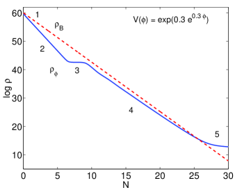
Figure 1: Evolution of the scalar field energy density $\rho_{\phi}$ in a radiation background fluid $\rho_{B}$ for a double exponential potential.

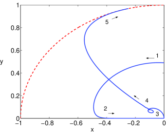
Figure 2: The scalar field dynamics in the phase space diagram for a double exponential potential. Regions 1 to 5 are the same as in Fig. 1. The dashed line represents the unit circle $x^{2}+y^{2}=1$.

The tracker solution. Consider the case in which the scalar field evolution is well approximated by a linear relation between $x$ and $y$ (region 4 in the figures). If we take the approximation of $\lambda$ large and $\Gamma$ nearly constant, then Eqs. (2) give the “instantaneous critical points”

$$x_{c}(\lambda)=\sqrt{\frac{3}{2}}\frac{\gamma_{\phi}}{\lambda}\,,\hskip 28.45274pty_{c}^{2}(\lambda)=\frac{3}{2}\frac{\gamma_{\phi}}{\lambda^{2}}(2-\gamma_{\phi})\,,$$ (7)

where the equation of state of the scalar field is

$$\gamma_{\phi}=\frac{1}{2}[\gamma+(2\Gamma-1)\frac{\lambda^{2}}{3}]-\frac{1}{2}\sqrt{\left[-\gamma+(2\Gamma-1)\frac{\lambda^{2}}{3}\right]^{2}+8\gamma(\Gamma-1)\frac{\lambda^{2}}{3}}\,.$$ (8)

This solution exists for $\lambda^{2}>3\gamma_{\phi}$.

The scalar contribution to the total energy density is $\Omega_{\phi}=3\gamma_{\phi}/\lambda^{2}$. Note that when $\Gamma-1\approx 0$ one has

$$\gamma_{\phi}=\gamma\left[1-\frac{2(\Gamma-1)}{1-3\gamma/\lambda^{2}}\right]\,.$$ (9)

In other words, for potentials with small curvature, the equation of state of the scalar field is very close to the equation of state of the background fluid, and it is said that the field “tracks” the background. This expression can account for values of $\Omega_{\phi}>1/2$.

From Eq. (8), it can also be shown that in the limit of $\lambda\rightarrow\infty$, when the background fluid is completely dominating, we recover the expression in [5],

$$\gamma_{\phi}=\frac{\gamma}{2\Gamma-1}.$$ (10)

The scalar field dominated solution. Consider now the case in which the evolution of the scalar field approaches the unit circle $x^{2}+y^{2}=1$ (region 5 in the figures). One can note that at late times $y\sim 1$ and $x\rightarrow 0$. This means that the scalar potential is overtaking the energy density and the potential is very flat. In other words, $\lambda$ is getting closer to zero. Let us take then $\lambda\approx 0$ and $\lambda^{2}(\Gamma-1)$ nearly constant. With these assumptions, we find critical points in,

$$x_{c}(\lambda)=\frac{\lambda_{\phi}}{\sqrt{6}}\,,\hskip 28.45274pty_{c}^{2}(\lambda)=1-\frac{\lambda_{\phi}^{2}}{6}\,.$$ (11)

Hence, the scalar field is dominant, $\Omega_{\phi}=1$ and $\gamma_{\phi}=\lambda_{\phi}^{2}/3$, where we have defined

$$\lambda_{\phi}=\frac{3}{2}\left[\frac{1-\sqrt{1-4(\Gamma-1)\lambda^{2}/3}}{(\Gamma-1)\lambda}\right],$$ (12)

for $\Gamma\neq 1$, and $\lambda_{\phi}=\lambda$ otherwise. Expanding $\lambda_{\phi}$ we can approximate the solution by

$$\lambda_{\phi}=\lambda\left[1+\frac{1}{3}(\Gamma-1)\lambda^{2}\right]\,.$$ (13)

This solution exists for $\lambda_{\phi}^{2}<6$.

We would like to stress that all the results presented in this talk are completely general, since no assumption on the shape of the potential was made in the calculation. A detailed discussion of the existence conditions and stability of the two attractors can be found in [1], together with an illustration of possible cosmological applications.

Acknowledgements.  It is a pleasure to thank N. J. Nunes and S. C. C. Ng with whom the work presented here was done.

References

- [1] S. C. Ng, N. J. Nunes and F. Rosati, Phys. Rev. D 64 (2001) 083510
- [2] E. J. Copeland, A. R. Liddle, and D. Wands, Phys. Rev. D57, 4686 (1998).
- [3] P. J. E. Peebles and B. Ratra, Astrophys. Jour. 325, L17 (1988); B. Ratra and P. J. E. Peebles, Phys. Rev. D37, 3406 (1988); A. R. Liddle and R. J. Scherrer, Phys. Rev. D59, 023509 (1999); S. C. C. Ng, Phys. Lett. 485, 1 (2000).
- [4] A. de la Macorra and G. Piccinelli, Phys. Rev. D61, 123503 (2000).
- [5] P. J. Steinhardt, L. Wang, and I. Zlatev, Phys. Rev. D59, 123504 (1999).
- [6] E. J. Copeland, N. J. Nunes and F. Rosati, Phys. Rev. D62, 123503 (2000).