Nonlinear magnetic diffusion and magnetic helicity transport in galactic dynamos

We have extended our previous mean-field galactic dynamo model which included algebraic and dynamic alpha nonlinearities (Kleeorin et al. 2002), to include also a quenching of turbulent diffusivity. We readily obtain equilibrium states for the large-scale magnetic field in the local disc dynamo model, and these fields have strengths that are comparable to the equipartition field strength. We find that the algebraic nonlinearity alone (i.e. quenching of both the $\alpha$ effect and turbulent magnetic diffusion) cannot saturate the growth of the mean magnetic field; only the combined effect of algebraic and dynamic nonlinearities can limit the growth of the mean magnetic field. However, in contrast to our earlier work without quenching of the turbulent diffusivity, we cannot now find satisfactory solutions in the no-$z$ approximation to the axisymmetric galactic dynamo problem.

1 Introduction

Spiral galaxies possess large-scale magnetic fields whose spatial scale is comparable with galactic radii (see for review Beck et al., 1996). Galactic magnetic fields mainly lie in the galactic plane and the corresponding magnetic lines are usually roughly of spiral form. This form can be substantially distorted in the presence of strong noncircular motions, e.g. in barred galaxies, see Beck et al. (1999, 2002), Moss et al.(2001).

Galactic magnetic fields are believed to originate in a galactic dynamo, driven by the joint action of the mean hydrodynamic helicity of interstellar turbulence and differential rotation. The linear stage of galactic dynamo action seems now to be well-understood, see, e.g., Ruzmaikin et al. (1988). The conventional approach to the nonlinear stage of the galactic dynamo is based on comparison of the relative intensity of three quantities participating in dynamo action, namely the differential rotation $\delta\Omega$, turbulent diffusivity $\eta_{T}$ and $\alpha$-effect, each of which can be associated with a typical velocity: $200$ km s^-1, $10$ km s^-1 and $1$ km s^-1 respectively. Because the typical velocity associated with $\alpha$ is the smallest, the mean hydrodynamic helicity is believed to be the weakest part of the self-excitation chain, and a scenario of nonlinear dynamo limitation via $\alpha$-quenching is the most commonly adopted.

A simple version of $\alpha$-quenching prescribes the mean hydrodynamic helicity to be a decreasing function of mean magnetic field strength $\bf B$. The critical magnetic field strength $B_{\rm cr}$, at which quenching becomes significant, is estimated conventionally from equipartition with the kinetic energy of interstellar turbulence, $B^{2}_{\rm eq}\sim 4\pi\rho v_{t}^{2}$. When applied to specific galaxies, this picture results in robust magnetic field models which are compatible with observations. However the picture is obviously oversimplified and various attempts to suggest a more developed version of nonlinear galactic dynamo theory have been undertaken by several authors. In particular, Vainstein and Cattaneo (1992) and Gruzinov and Diamond (1995) have claimed that in fact $B_{\rm cr}$ is much lower then the equipartition value, e.g. $B_{\rm cr}=B_{\rm eq}Rm^{-1/2}$, where $Rm$ is the magnetic Reynolds number. In galaxies, magnetic Reynolds numbers are very large, $Rm\approx 10^{6}$ even if the ambipolar diffusivity coefficient is used, so it was claimed that dynamo action saturates at a magnetic field strength that is much lower than both the equipartition value, and also the large-scale field strengths observed in nearby spiral galaxies. This result follows from investigations that accept the idea of magnetic helicity conservation. The galactic dynamo produces a large-scale magnetic field with nonvanishing magnetic helicity, and when considering detailed magnetic helicity conservation in a given volume, the above ‘catastrophic’ estimate for $B_{\rm cr}$ results.

The evolution of magnetic helicity appears however to be a more complicated process than can simply be described by a balance of magnetic helicity in a given volume, and it is necessary to take into account, as for the evolution of other conserved quantities, transport by the fluid flows including turbulent transport of magnetic helicity through the galactic boundaries and the destruction of mean magnetic helicity by turbulent diffusion. The governing equation for magnetic helicity was suggested by Kleeorin & Ruzmaikin (1982; see also the discussion by Zeldovich et al. 1983) for an isotropic turbulence, and investigated by Kleeorin et al. (1995) for stellar dynamos, and self-consistently derived by Kleeorin & Rogachevskii (1999) for an arbitrary anisotropic turbulence. A quantitative model for the flux of magnetic helicity was proposed by Kleeorin & Rogachevskii (1999) and Kleeorin et al. (2000). Note that Schmalz & Stix (1991), Covas et al. (1998) and Blackman & Brandenburg (2002) have also investigated related solar dynamo models that included a dynamical equation describing the evolution of magnetic helicity. Magnetic helicity transport through the boundary of a dynamo region is reported by Chae (2001) to be observable at the solar surface. The role of a flux of magnetic helicity in the dynamics of the mean magnetic field in accretion discs was also discussed by Vishniac & Cho (2001).

The equation governing the magnetic helicity is much more complex than the conventional parametrization used to represent $\alpha$-quenching. Kleeorin et al. (2000) suggested that a nonlinear galactic dynamo governed by a consistently derived equation for magnetic helicity results in a steady magnetic field comparable with the equipartition magnetic field estimate, and Kleeorin et al. (2002) demonstrated that a detailed galactic dynamo model based on the equation under discussion gives results very similar to one based on conventional $\alpha$-quenching. In other words, the real physical description of the nonlinear stage of galactic dynamo is quite complicated but, if we are interested in pragmatic results only, an adequate description can be found by using only a conventional $\alpha$-quenching.

We stress that the scenario of Kleeorin et al. (2000, 2002) does not include all possible types of nonlinear processes which can occur at the nonlinear dynamo stage (see, e.g., Brandenburg & Subramanian 2000; Brandenburg & Dobler 2001), but rather is restricted by a minimal number of processes involved in the magnetic helicity conservation. In particular, we consider transport of mean helicity of small-scale magnetic field only and note that this helicity may be transported out of the galactic disc without significant losses of large-scale magnetic field. Moreover, this picture is formulated in terms of mean-field electrodynamics, which gives a natural constraint on the description of small-scale details. When attention is focussed on these details (e.g. Brandenburg & Sokoloff 2002; Blackman & Brandenburg 2002), the mean-field description should be considered as a parametrization of the turbulence.

In the spirit of the basic ideas about the nonlinear saturation of galactic dynamos, the analysis presented by Kleeorin et al. (2000, 2002) was restricted to the evolution of $\alpha$ only, while a detailed simulation (e.g. Brandenburg & Sokoloff 2002) also demonstrates a quenching of the turbulent magnetic diffusivity. A quantitative model for a nonlinear quenching of turbulent magnetic diffusivity has been recently suggested by Rogachevskii & Kleeorin (2001).

The aim of the present paper is to include a turbulent magnetic diffusivity quenching into the mean-field dynamo equations. This effect is expected to be quite modest. Speaking pragmatically, we do not know the turbulent magnetic diffusivity of interstellar turbulence well enough to recognize its saturation, by some dozens of percent. However, our analysis below demonstrates that the problem is not restricted by some specific variation of magnetic diffusivity coefficient. Because of nonlinear effects, the turbulent magnetic diffusion coefficients for the two basic magnetic field components, i.e. poloidal and toroidal, become different (see Rogachevskii & Kleeorin 2001). Since spatial magnetic field distribution is nonuniform, a nonuniform magnetic diffusivity saturation arises, that results in new terms in the dynamo equations governing the nonlinear magnetic field evolution. In general, the situation appears to be less trivial then might be thought initially, and a quantitative analysis of a specific dynamo model becomes desirable. Below we present results of the corresponding analysis and numerical simulations.

2 The mean-field equations

The mean-field dynamo equation (e.g. Krause & Rädler 1980) is

$$\frac{\partial{\@vec{B}}}{\partial t}=\@vec{\nabla}{\bf\times}(\@vec{V}{\bf\times}\@vec{B}+\@vec{\cal E}-\eta\,\@vec{\nabla}{\bf\times}\@vec{B})\;,$$ (1)

where ${\bf V}$ is a mean velocity (e.g., the differential rotation), $\eta$ is the magnetic diffusion due to the electrical conductivity of fluid together with ambipolar diffusion, $\@vec{\cal E}=\langle{\bf u}\times{\bf b}\rangle$ is the mean electromotive force, ${\bf u}$ and ${\bf b}$ are fluctuations of the velocity and magnetic field, respectively, angular brackets denote averaging over an ensemble of fluctuations. When a small-scale background turbulence (i.e. turbulence with a zero mean magnetic field) is isotropic and the energy of small-scale magnetic fluctuations of the background turbulence is much smaller than that of the kinetic energy, the mean electromotive force is given by

$${\cal E}_{i}=\alpha_{ij}(\@vec{B})B_{j}+(\@vec{V}^{\rm eff}(\@vec{B}){\bf\times}\@vec{B})_{i}-\eta_{ij}(\@vec{B})(\@vec{\nabla}{\bf\times}\@vec{B})_{j}\;,$$ (2)

where

$$\eta_{ij}(\@vec{B}) = [\eta_{A}(\@vec{B})-\eta_{\beta}(\@vec{B})]\,\delta_{ij}+\eta_{\beta}(\@vec{B})\,B_{ij}\;,$$ (3)

$$\@vec{V}^{\rm eff}(\@vec{B}) = {1\over 2}\eta_{V}(\@vec{B}){\@vec{\nabla}B^{2}\over B^{2}}\;,$$ (4)

(see Rogachevskii & Kleeorin, 2001), $B_{ij}=B_{i}B_{j}/B^{2},$ $\,\alpha_{ij}(\@vec{B})=\alpha(\@vec{B})\delta_{ij},$ $\,\eta_{V}(\@vec{B})=\eta_{A}(\@vec{B})-\eta_{B}(\@vec{B})-\eta_{\beta}(\@vec{B})$ and $\alpha(\@vec{B})$, $\,\eta_{A}(\@vec{B}),$ $\,\eta_{B}(\@vec{B})$, $\,\eta_{\beta}(\@vec{B})$ are determined by Eqs. (8), (11), (12) and (14), respectively.

2.1 The local thin-disc dynamo problem

We begin by considering the simplest local disc dynamo problem. Using cylindrical polar coordinates $r,\phi,z$, from Eqs. (1)-(4) we obtain the equations for the mean radial field $B_{r}=R_{\alpha}b_{r}$ and toroidal field $B_{\phi}$ for the local thin-disc axisymmetric $\alpha\Omega$-dynamo problem as

$${{\partial b_{r}}\over{\partial t}} = -(\alpha(\@vec{B})B_{\phi})^{\prime}+(\eta_{A}(\@vec{B})b_{r}^{\prime})^{\prime}-(V_{A}(\@vec{B})b_{r})^{\prime}\;,$$ (5)

$${{\partial B_{\phi}}\over{\partial t}} = Db_{r}+(\eta_{B}(\@vec{B})B^{\prime}_{\phi})^{\prime}\;$$ (6)

(Ruzmaikin et al. 1988, Rogachevskii & Kleeorin 2001). Here a prime denotes $\partial/\partial z,$ $\alpha(\@vec{B})$ is the total nonlinear $\alpha$ effect, $\eta_{A}(\@vec{B})$ and $\eta_{B}(\@vec{B})$ are the nonlinear turbulent magnetic diffusion coefficients of poloidal and toroidal mean magnetic fields, and the nonlinear function $V_{A}(\@vec{B})\equiv[\eta_{A}(\@vec{B})-\eta_{B}(\@vec{B})](\ln B)^{\prime}$, with $B=|\@vec{B}|.$ These nonlinearities are specified and discussed in the next Section.

We adopt here the standard dimensionless form of the galactic dynamo equations from Ruzmaikin et al. (1988); in particular, length is measured in units of the disc thickness $h$, time in units of $h^{2}/\eta_{T}$ and $B$ is measured in units of the equipartition energy $B_{\rm eq}=\sqrt{4\pi\rho}\,u_{\ast}$, $\alpha$ is measured in units of $\alpha_{\ast}$ (the maximum value of the hydrodynamic part of the $\alpha$ effect), the nonlinear turbulent magnetic diffusion coefficients $\eta_{A}(\@vec{B})$ and $\eta_{B}(\@vec{B})$ are measured in units of $\eta_{T}$. We define $R_{\alpha}=h\alpha_{\ast}/\eta_{T},$ $\,R_{\omega}=r\,(d\Omega/dr)\,h^{2}/\eta_{T}$, and the dynamo number $D=R_{\omega}R_{\alpha}$, where $l$ is the maximum scale of the turbulent motions, $Rm=lu_{\ast}/\eta$ is the magnetic Reynolds number. Also $u_{\ast}$ is the characteristic turbulent velocity at the scale $l$, $\rho$ is the gas density, and the characteristic value of the turbulent magnetic diffusivity $\eta_{T}=lu_{\ast}/3$.

Throughout this paper, unless otherwise stated, we measure magnetic field in units of the equipartition value. Here we assumed that the background turbulence (i.e., the turbulence with a zero mean magnetic field) is isotropic and has only velocity fluctuations, even though a nonzero mean magnetic field can be expected to produce an anisotropy of turbulence from the generated magnetic fluctuations.

3 The nonlinearities

3.1 The nonlinear $\alpha$ effect

The total nonlinear $\alpha$ effect is given by

$$\alpha(\@vec{B})=\alpha^{v}+\alpha^{m}\;,$$ (7)

where $\alpha^{v}$ is the hydrodynamic part of the $\alpha$ effect, and $\alpha^{m}$ is the magnetic part of the $\alpha$ effect. These quantities are determined by the corresponding helicities and quenching functions, $\phi_{v}(B)$ and $\phi_{m}(B).$ In particular, $\alpha^{v}=\chi^{v}\phi_{v}(B),$ $\alpha^{m}=\chi^{c}(\@vec{B})\phi_{m}(B)$ and $\chi^{v}=-(\tau/3)\langle\leavevmode\nobreak\ \@vec{u}\leavevmode\nobreak\ \cdot\leavevmode\nobreak\ (\@vec{\nabla}{\bf\times}\@vec{u})\leavevmode\nobreak\ \rangle,$ $\;\chi^{c}\equiv(\tau/12\pi\rho)\langle\@vec{b}\cdot(\@vec{\nabla}{\bf\times}\@vec{b})\rangle$ is related with current helicity, where $\tau$ is the correlation time of turbulent velocity field and $\langle\@vec{u}\cdot(\@vec{\nabla}{\bf\times}\@vec{u})\rangle$ is the hydrodynamic helicity. Thus,

$$\alpha(\@vec{B})=\chi^{v}\phi_{v}(B)+\chi^{c}(\@vec{B})\phi_{m}(B)\;,$$ (8)

where the quenching functions $\phi_{v}(B)$ and $\phi_{m}(B)$ are given by

$$\phi_{v}(B) = (1/7)[4\phi_{m}(B)+3L(\sqrt{8}B)]\;,$$ (9)

$$\phi_{m}(B) = (3/\beta^{2})(1-\arctan(\beta)/\beta)\;$$ (10)

(see Rogachevskii & Kleeorin, 2000), where $\beta=\sqrt{8}B$ and $L(\beta)=1-2\beta^{2}+2\beta^{4}\ln(1+\beta^{-2}).$ Thus $\phi_{v}(B)=2/\beta^{2}$ and $\phi_{m}(B)=3/\beta^{2}$ for $\beta\gg 1;$ and $\phi_{v}(B)=1-(6/5)\beta^{2}$ and $\phi_{m}(B)=1-(3/5)\beta^{2}$ for $\beta\ll 1.$ The function $\chi^{c}(\@vec{B})$ entering the magnetic part of the $\alpha$ effect is determined by the dynamical equation (15). Here $\chi^{v}$ and $\chi^{c}$ are measured in units of $\alpha_{\ast}$.

The function $\phi_{v}(B)$ describes conventional quenching of the $\alpha$ effect. A simple form of such a quenching, $\phi_{v}=1/(1+B^{2}),$ was introduced long ago (see, e.g., Iroshnikov, 1970). The splitting of the total $\alpha$ effect into the hydrodynamic ($\alpha^{v}$) and magnetic ($\alpha^{m}$) parts was first suggested by Frisch et al. (1975). The magnetic part $\alpha^{m}$ includes two types of nonlinearity: the algebraic quenching described by the function $\phi_{m}(B)$ (see e.g. Field et al. 1999; Rogachevskii & Kleeorin 2000, 2001) and the dynamic nonlinearity which is determined by Eq. (15).

3.2 Nonlinear turbulent magnetic diffusion coefficients of the toroidal and poloidal mean magnetic fields

The nonlinear turbulent magnetic diffusion coefficients of poloidal and toroidal mean magnetic fields $\eta_{A}(B)$ and $\eta_{B}(B)$, and the nonlinear function $V_{A}(B)\equiv[\eta_{A}(B)-\eta_{B}(B)](\ln B)^{\prime}$ are given in dimensionless form by

$$\eta_{A}(B) = A_{1}(\sqrt{2}\beta)+(1/2)A_{2}(\beta)\;,$$ (11)

$$\eta_{B}(B) = A_{1}(\sqrt{2}\beta)-(1/2)A_{2}(\beta)+A_{2}(\sqrt{2}\beta)$$ (12)

$$+(\beta/\sqrt{2})\Psi(\sqrt{2}\beta)\;,$$

$$V_{A}(B) = [A_{2}(\beta)-A_{2}(\sqrt{2}\beta)$$ (13)

$$-(\beta/\sqrt{2})\Psi(\sqrt{2}\beta)](\ln B)^{\prime}\;,$$

(see Rogachevskii & Kleeorin, 2001), where $\Psi(x)=(d/dx)[A_{1}(x)+(1/2)A_{2}(x)],$ and

$$\eta_{\beta}(\@vec{B})=(1/2)A_{2}(\beta)\;.$$ (14)

The functions $A_{1}(\beta)$ and $A_{2}(\beta)$ are given by

$$A_{1}(\beta) = {6\over 5}\biggl{[}{\arctan\beta\over\beta}\biggl{(}1+{5\over 7\beta^{2}}\biggr{)}+{1\over 14}L(\beta)-{5\over 7\beta^{2}}\biggr{]}\;,$$

$$A_{2}(\beta) = -{6\over 5}\biggl{[}{\arctan\beta\over\beta}\biggl{(}1+{15\over 7\beta^{2}}\biggr{)}-{2\over 7}L(\beta)-{15\over 7\beta^{2}}\biggr{]}\;.$$

When $\beta\ll 1$ these functions are given approximately by

$$A_{1}(\beta) = 1-(2/5)\beta^{2}\;,\quad A_{2}(\beta)=-(4/5)\beta^{2}\;,$$

and for $\beta\gg 1$ they are given by

$$A_{1}(\beta) = 3\pi/5\beta-4/5\beta^{2}\;,\quad A_{2}(\beta)=-3\pi/5\beta+14/5\beta^{2}\;.$$

The asymptotic formulas for the functions $\eta_{A}(B),$ $\eta_{B}(B)$ and $V_{A}(B)$ for $\beta\ll 1$ are

$$\eta_{A}(B) = 1-(6/5)\beta^{2}\;,\quad\eta_{B}(B)=1-(18/5)\beta^{2}\;,$$

$$V_{A}(B) = (12/5)\beta^{2}(\ln B)^{\prime}\;,$$

and for $\beta\gg 1$

$$\eta_{A}(B) = {3\pi\over 10\beta}(\sqrt{2}-1)\;,$$

$$\eta_{B}(B) = {3\pi\over 20\beta}(2-{1\over\sqrt{2}})\;,$$

$$V_{A}(B) = -{3\pi\over 5\beta}(1-{5\sqrt{2}\over 8})(\ln B)^{\prime}\;.$$

The quenching of the $\alpha$ effect and the turbulent magnetic diffusion are caused by the direct and indirect modification of the electromotive force by the mean magnetic field. The indirect modification of the electromotive force is caused by the effect of the mean magnetic field on the velocity fluctuations (described by the tensors $\langle u_{i}u_{j}\rangle$) and on the magnetic fluctuations (determined by the tensor $\langle b_{i}b_{j}\rangle),$ while the direct modification is due to the effect of the mean magnetic field on the cross-helicity tensor $\langle u_{i}b_{j}\rangle$ (see, e.g., Rogachevskii & Kleeorin 2000, 2001).

3.3 The dynamical equation for the function $\chi^{c}(\@vec{B})$

The function $\chi^{c}(\@vec{B})$ entering the magnetic part of the $\alpha$ effect is determined by the dynamical equation

$${{\partial\chi^{c}}\over{\partial t}} = -4\biggl{(}{h\over l}\biggr{)}^{2}[\@vec{\cal E}{\bf\cdot}\@vec{B}+\@vec{\nabla}\cdot\@vec{F}]-\@vec{\nabla}\cdot[\@vec{V}\chi^{c}$$ (15)

$$-\kappa\@vec{\nabla}\chi^{c}]-\chi^{c}/T\;,$$

where $\@vec{F}=C\chi^{v}\phi_{v}(B)\@vec{B}^{2}\eta_{A}(\@vec{B})(\@vec{\nabla}\rho)/\rho$ is the nonadvective flux of the magnetic helicity which serves as an additional nonlinear source in the equation for $\chi^{c}$, $\,\@vec{V}\chi^{c}$ is the advective flux of the magnetic helicity and $-\kappa\@vec{\nabla}\chi^{c}$ is the diffusive flux of the magnetic helicity (see Kleeorin & Rogachevskii, 1999; Kleeorin et al. 2000; 2002), $\,\@vec{V}=\@vec{e}_{\phi}\,\Omega\,r$ is the differential rotation, and $T=(1/3)(l/h)^{2}Rm$. Eq. (15) was obtained using arguments based on the magnetic helicity conservation law (see Kleeorin & Rogachevskii, 1999). The function $\chi^{c}$ is proportional to the magnetic helicity, $\chi^{c}=\chi^{m}/(18\pi\eta_{T}\rho)$ (see e.g. Kleeorin & Rogachevskii, 1999), where $\chi^{m}=\langle\@vec{a}\cdot\@vec{b}\rangle$ is the magnetic helicity and $\@vec{a}$ is the vector potential of small-scale magnetic field. Here we assume that the helical part of the vector potential $\@vec{a}$ is a locally isotropic and homogeneous random field, which is a natural gauge condition used in our approach. Thus, Eq. (15) describes the evolution of magnetic helicity, i.e. its production, dissipation and transport.

The turbulent diffusion of the magnetic helicity $\kappa$ plays an important role and can be interpreted as follows. The random flows existing in the interstellar medium consist of a combination of small-scale motions, which are affected by magnetic forces resulting in a steady-state of the dynamo, and a microturbulence which is supported by a strong random driver (supernovae explosions) which can be considered as independent of the galactic magnetic field. The large-scale magnetic field is smoothed over both kinds of turbulent fluctuations, while the small-scale magnetic field is smoothed over microturbulent fluctuations only. It is the smoothing over the microturbulent fluctuations that gives the coefficient $\kappa$.

For galaxies the relaxation term $\chi^{c}/T$ is very small and can be dropped in spite of the fact the small yet finite magnetic diffusion is required for the reconnection of magnetic field lines. For example, we will show below that the magnetic Reynolds number, $Rm,$ does not enter into the steady state solution of Eq. (15) in the limit of very large $Rm$, because of the effect of the magnetic helicity flux. In particular, keeping the term $\chi^{c}/T$ we obtain from Eq. (15) that in a steady state

$$\alpha={\alpha_{v}+\tau_{\ast}\,Rm\,\phi_{m}(\@vec{B})\,[\@vec{B}\cdot(\@vec{\nabla}{\bf\times}\@vec{B})-{\rm div}\,\@vec{F}_{t}]\over 1+\tau_{\ast}\,Rm\,\phi_{m}(\@vec{B})\,B^{2}}\;,$$ (16)

where $\tau_{\ast}=l/u_{\ast}$ and $\@vec{F}_{t}=\@vec{F}+\@vec{V}\chi^{c}-\kappa\nabla\chi^{c}$ is the total flux of the magnetic helicity. In the limit of very large $Rm,$ Eq. (16) reads

$$\alpha={\@vec{B}\cdot(\@vec{\nabla}{\bf\times}\@vec{B})-{\rm div}\,\@vec{F}_{t}\over B^{2}}\;.$$ (17)

This implies that in this limit the total $\alpha$ is independent of the magnetic Reynolds number.

In the local approximation Eq. (15) reads:

$${\partial\chi^{c}\over\partial t} = 4\biggl{(}{h\over l}\biggr{)}^{2}[\eta_{A}(\@vec{B})(B_{\phi}b^{\prime}_{r}-B^{\prime}_{\phi}b_{r})-\alpha(\@vec{B})B^{2}$$ (18)

$$+C{{\partial}\over{\partial z}}(|\chi^{v}(z)|\phi_{v}(B)B^{2}\eta_{A}(\@vec{B}))]+(\kappa(\chi^{c})^{\prime})^{\prime}\;.$$

Here we do not take into account any inhomogeneity of the turbulent magnetic diffusion at ${\bf B}=0$. The turbulent magnetic diffusion is inhomogeneous due to inhomogeneity of the mean magnetic field ${\bf B}$.

The turbulent magnetic diffusion $\kappa$ of the magnetic helicity (and the function $\chi^{c})$ can depend on the mean magnetic field. The nonlinear quenching of the turbulent magnetic diffusion of the magnetic helicity is given by $\phi_{\kappa}(B)$,

$$\phi_{\kappa}(B)={1\over 2}\biggl{[}1+A_{1}(\sqrt{2}\beta)+{1\over 2}A_{2}(\sqrt{2}\beta)\biggr{]}\;.$$ (19)

For $\beta\ll 1$ we have approximately

$$\phi_{\kappa}(B)=1-{3\over 5}\beta^{2}\;,$$

and for $\beta\gg 1$ we have

$$\phi_{\kappa}(B)={1\over 2}\biggl{(}1+{3\pi\over 10\sqrt{2}\beta}\biggr{)}\;.$$

The turbulent magnetic diffusion $\kappa(B)$ of the magnetic helicity is determined by the tensor $\tau\langle u_{i}u_{j}\rangle.$ Thus, Eqs (8), (11)–(13) and (18) contain the main nonlinearities.

4 Equilibrium states of the local dynamo model

4.1 Asymptotic expansions and an equilibrium solution

We now present asymptotic expansions for a galactic dynamo model determined by Eqs. (5), (6) and (18). For the $\alpha\Omega$-dynamo $B\approx B_{\phi}.$ This assumption is justified if $|D|\gg R_{\alpha},$ i.e. $|R_{\omega}|\gg 1.$ In a steady-state for fields of even parity with respect to the disc plane, Eqs. (5), (6) and (18) with $\kappa=0$ gives

$$[\eta_{B}(B)B^{\prime}]^{2}+2CD\phi_{v}(B)\eta_{A}(B)B^{2}|\chi^{v}(z)|=0\;.$$ (20)

The solution of Eq. (20) for negative $D$ is given by

$$\int_{0}^{B}G(\tilde{B})\,d\tilde{B}=\sqrt{2C|D|}\int_{|z|}^{1}\sqrt{|\chi^{v}(\tilde{z})|}\,d\tilde{z}\;,$$ (21)

where $G(B)=\eta_{B}(B)/[\phi_{v}(B)\eta_{A}(B)B^{2}]^{1/2}.$ For an arbitrary profile $|\chi^{v}(z)|$, negative dynamo number $D$ and for $B\gg 1/\sqrt{8},$ there is an explicit steady solution of this equation with the boundary conditions $B_{\phi}(z=1)=0$ and $B_{\phi}^{\prime}(z=0)=0$,

$$B(z)\approx(2/5)C|D|\biggl{(}\int_{|z|}^{1}\sqrt{|\chi^{v}(\tilde{z})|}\,d\tilde{z}\biggr{)}^{2}\;,$$ (22)

where $z$ is measured in the units of $h,$ and we have used that for $B\gg 1/\sqrt{8}$ we have $\eta_{A}(B)\sim 2/5\beta,$ $\eta_{B}(B)\sim 3/5\beta,$ $\phi_{v}(B)\sim 2/\beta^{2}.$ Here $\beta=\sqrt{8}B.$ In a steady state $b_{r}(z)=(\eta_{B}(B)B^{\prime})^{\prime}/|D|.$ For the specific choice of the profile $|\chi^{v}(z)|=\sin^{2}(\pi z/2)$ we obtain

$$B_{\phi} \approx {4\over 25}C\,|D|\,B_{\rm eq}\cos^{2}\,\biggl{(}{{\pi z}\over 2}\biggr{)}\;,$$ (23)

$$B_{r} \approx -{1\over|R_{\omega}|}B_{\rm eq}\cos^{-2}\,\biggl{(}{{\pi z}\over 2}\biggr{)}\;,$$ (24)

where we have now restored the dimensional factor $B_{\rm eq}.$ The boundary conditions for $B_{r}$ are $B_{r}(z=1)=0$ and $B_{r}^{\prime}(z=0)=0.$ Note, however, that our asymptotic analysis performed for $B\gg 1/\sqrt{8}$ is not valid in the vicinity of the point $z=1$ because $B(z=1)=0$.

4.2 Numerical solutions for the one-dimensional model

We found solutions of Eqs. (5), (6) and (18) by step by step integration, from arbitrarily chosen initial conditions. Various properties of the solutions for the mean magnetic field and the z-profiles of the main nonlinearities – the $\alpha$–effect, turbulent magnetic diffusion of the toroidal and poloidal fields – are illustrated in Figs. 1 – 6. It can be seen clearly that the field strength ($\sim|B_{\phi}|$) is typically of order 1 (equipartition), and increases with $|D|$.

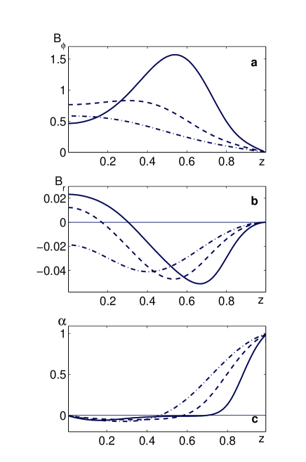
Figure 1: The $z$-dependence of solutions for the local model; $h/l=5$; $C=-0.1$, $\kappa=0.3$ and $|\chi^{v}(z)|=\sin^{2}(\pi z/2)$. The various curves indicate results with dynamo numbers $D=-20$ (dashed-dotted), $D=-40$ (dashed) and $D=-100$ (solid). a) the toroidal magnetic field $B_{\phi}(z)$, b) the poloidal magnetic field $B_{r}(z)$, c) the total $\alpha$-effect, $\alpha(z)$.

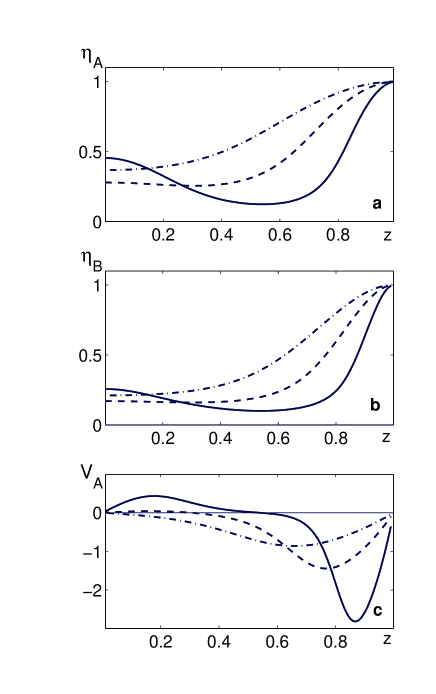
Figure 2: As Fig. 1. The functions: a) $\eta_{A}(z)$, b) $\eta_{B}(z)$, c) $V_{A}(z)$.

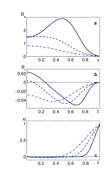
Figure 3: As Fig. 1, with $C=0.1$.

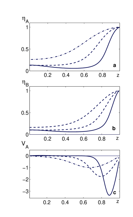
Figure 4: As Fig. 2, with $C=0.1$.

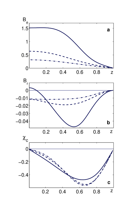
Figure 5: The $z$-dependence of solutions for the local model; $h/l=5$; $C=0.1$, $D=-40$ and $|\chi^{v}(z)|=\sin^{2}(\pi z/2)$. The various curves indicate results with $\kappa=0.05$ (dashed-dotted), $\kappa=0.1$ (dashed) and $\kappa=0.3$ (solid). a) the toroidal magnetic field $B_{\phi}(z)$, b) the poloidal magnetic field $B_{r}(z)$, c) the function $\chi^{c}(z)$.

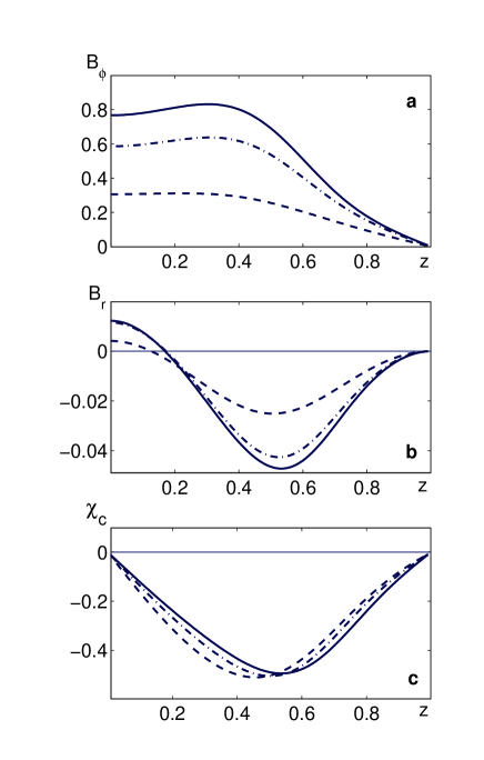
Figure 6: The $z$-dependence of solutions for the local model; $h/l=5$; $C=-0.1$, $D=-40$ and $|\chi^{v}(z)|=\sin^{2}(\pi z/2)$. The various curves indicate results without $\kappa$-quenching for $\kappa=0.1$ (dashed) and $\kappa=0.3$ (solid) and with $\kappa$-quenching for $\kappa=0.3$ (dashed-dotted). a) the toroidal magnetic field $B_{\phi}(z)$, b) the poloidal magnetic field $B_{r}(z)$, c) the function $\chi^{c}(z)$.

New features were found in comparison with the results of Kleeorin et al. (2002), where the quenching of the turbulent magnetic diffusion was not taken into account. In particular, the maximum of the toroidal magnetic field for $|D|>40$ is not located at $z=0$ but is shifted to $z\approx 0.5h$ (see Figs. 1a and 3a). The equipartition toroidal field is attained for smaller values of the dynamo numbers and parameter $C$ than in the model studied by Kleeorin et al (2002). The reason is that the asymptotic behavior of the steady-state solution is different in these two cases: in the present study $B_{\phi}\propto C\,|D|\,B_{\rm eq}$ (see Eq. (23)) whereas when the quenching of the turbulent magnetic diffusion vanishes we have $B_{\phi}\propto\sqrt{C\,|D|}\,B_{\rm eq}$ (see Eq. (18) in Kleeorin et al., 2002). Note that for galaxies reasonable estimates are $|D|\sim 10-30$, $\,|C|\sim 0.1$ and $\kappa\sim 0.3-0.5.$ With these parameters the present model gives toroidal field strengths of about the equipartition value.

Fig. 2c demonstrates the change of sign of the effective drift velocity with $z,$ so that in one part of the disc it is diamagnetic, and in the other it is paramagnetic. A diamagnetic velocity implies that the field is pushed out from regions with stronger mean magnetic field, while a paramagnetic velocity causes the magnetic field to be concentrated in regions with stronger field.

Fig. 6 shows the solutions for different values of the turbulent diffusion $\kappa$ of the magnetic helicity. It is apparent from Fig. 6 that the magnitude of the saturated toroidal magnetic field increases with $\kappa.$ The reason is clear; the increase of this parameter increases the flux of the magnetic helicity, and causes a decrease of the magnetic part of the $\alpha$–effect, thus increasing the total $\alpha$–effect.

When comparing the numerical and asymptotic solutions we need to take into account that the asymptotic solution (23)–(24) was obtained only for $\kappa=0.$ Thus such a comparison can only be performed for very small values of $\kappa.$ If we compare the field $B_{\phi}$ at $z=0$ for, e.g., $C=0.1$ and $\kappa=0.05$ we find that the difference between the asymptotic and numerical solutions is about 15 percent when $D=-100.$ The novel feature, the maximum of the toroidal field $B_{\phi}$ at $z>0$ rather than $z=0$, appears in the numerical solutions for $\kappa\geq 0.1$, and is not described in the framework of the above asymptotic analysis. Note also that a discrepancy between the numerical and asymptotic solutions is perhaps not so surprising even for large values of $|D|$, as relation (24) diverges near $z=1.$

In order to separate the study of the algebraic and dynamic nonlinearities we define a function $D_{V}(B)/D=\phi_{v}(B)/[\eta_{A}(B)\eta_{B}(B)]$, using only the hydrodynamic part of the $\alpha$ effect. Thus, for $B\gg 1/\sqrt{8}$ the function $D_{V}(B)/D$ is a nonzero constant, because then $\eta_{A}(B)\sim 2/5\beta,$ $\eta_{B}(B)\sim 3/5\beta,$ $\phi_{v}(B)\sim 2/\beta^{2}$, with $\beta=\sqrt{8}B.$ The saturation of the growth of the mean magnetic field in the case with only an algebraic nonlinearity present can be achieved when the derivative of the function $dD_{V}(B)/dB<0.$ Thus, taking into account quenching of the turbulent magnetic diffusion we find that the algebraic nonlinearity alone (i.e. quenching of both the $\alpha$ effect and turbulent magnetic diffusion) cannot saturate the growth of the mean magnetic field because $dD_{V}(B)/dB\to 0$ for $B\gg 1/\sqrt{8}$.

We will show here that the combined effect of the algebraic and dynamic nonlinearities limits the growth of the mean magnetic field. The dynamic nonlinearity is determined by the evolutionary equation (18) for $\chi^{c}$. We introduce the parameter $D_{N}(B)/D=\alpha(B)/[\alpha(B=0)\eta_{A}(B)\eta_{B}(B)]$ which characterizes both the algebraic and dynamic nonlinearities, while the parameter $D_{V}(B)/D$ characterizes only the algebraic nonlinearity. The saturation of the growth of the mean magnetic field is achieved when the derivative of the nonlinear dynamo number satisfies $dD_{N}(B)/dB<0.$ We see in Fig. 7 that this condition is satisfied. However, we see also that $dD_{V}(B)/dB>0.$ This implies that the algebraic nonlinearity alone (i.e. quenching of both the $\alpha$ effect and turbulent magnetic diffusion) cannot saturate the growth of the mean magnetic field. The same follows from the above asymptotic analysis.

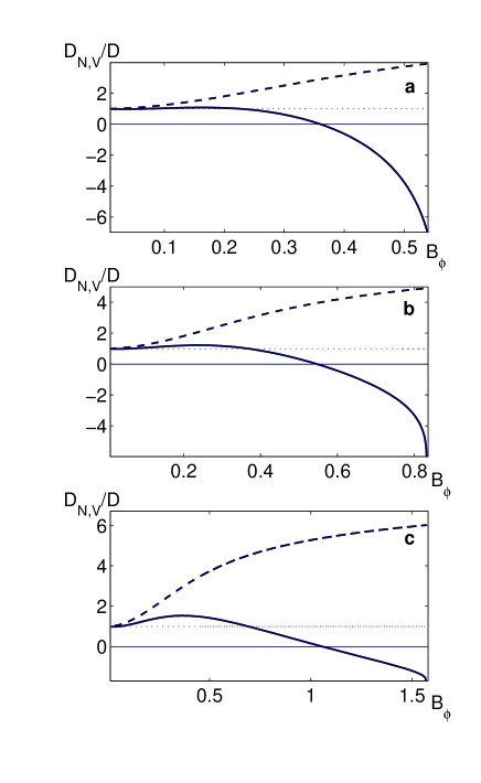
Figure 7: The dependencies of $D_{N}(B)/D=\alpha(B)/[\alpha(B=0)\eta_{A}(B)\eta_{B}(B)]$ (solid) and $D_{V}(B)/D=\phi_{v}(B)/[\eta_{A}(B)\eta_{B}(B)]$ (dashed) on the mean magnetic field for the one-dimensional model; $h/l=5$; $C=-0.1$; $\kappa=0.3$; with different $D$: a) $D=-20$; b) $D=-40$; c) $D=-100$.

5 Simple models with radial extent

Detailed numerical modelling of galactic dynamos is quite a complicated numerical problem. Dynamo models with conventional $\alpha$-quenching are however very robust and allow drastic simplifications that nevertheless reproduce adequately the basic features of galactic magnetic field structure as reflected in the observational data. The aim of this section is to discuss to what extent these simplified models are comparable with the quenching discussed above.

The basic no-$z$ dynamo model for disc galaxies has proved to be a useful tool for studying dynamo action in these objects, and is described in Moss (1995). Here we also include the tuning suggested by Phillips (2001), namely the multiplication by factors $f=\pi^{2}/4$ of the terms representing the $z$-diffusion of $B_{r}$ and $B_{\phi}$. The no-$z$ model differs from the local model of Sect. 2.1 in that it describes magnetic fields over the entire radial range, $0\leq r\leq R$, but all explicit dependence on the vertical coordinate $z$ has been removed, with the first-order $z$-derivatives being replaced by $1/h$ and the second-order $z$-derivatives being replaced by $-f/h^{2}$. The field components $B_{r}$, $B_{\phi}$ appearing in the no-$z$ equations can either be thought of as representing mid-plane values, or as some sort of vertical average of values through the disc.

For the no-z model in the axisymmetric case the mean-field dynamo equations take the form

$${\partial B_{\phi}\over\partial t} = -f\eta_{B}\biggl{(}{B\over\sqrt{\rho}}\biggr{)}B_{\phi}$$ (25)

$$+\lambda^{2}{\partial\over\partial r}\biggl{[}\eta_{B}\biggl{(}{B\over\sqrt{\rho}}\biggr{)}{1\over r}{\partial\over\partial r}(rB_{\phi})\biggr{]}$$

$$+R_{\omega}B_{r}r{\partial\Omega\over\partial r}+\lambda^{2}{\partial\over\partial r}\biggl{[}\eta_{V}\biggl{(}{B\over\sqrt{\rho}}\biggr{)}{B\over r}\biggr{]}\;,$$

$${\partial B_{r}\over\partial t} = -R_{\alpha}\alpha B_{\phi}-\biggl{[}(f+1)\eta_{A}\biggl{(}{B\over\sqrt{\rho}}\biggr{)}$$ (26)

$$-\,\eta_{B}\biggl{(}{B\over\sqrt{\rho}}\biggr{)}\biggr{]}B_{r}+\lambda^{2}\eta_{A}\biggl{(}{B\over\sqrt{\rho}}\biggr{)}{\partial\over\partial r}\biggl{(}{1\over r}{\partial\over\partial r}(rB_{r})\biggr{)}$$

$$-\lambda^{2}\tilde{V}_{A}\biggl{(}{B\over\sqrt{\rho}}\biggr{)}{1\over r}{\partial\over\partial r}(rB_{r})\;.$$

$${\partial\chi^{c}\over\partial t} = {1\over\rho(r)}\biggl{\{}4\biggl{(}{h\over l}\biggr{)}^{2}\biggl{[}C\,\chi^{v}\,\eta_{A}\biggl{(}{B\over\sqrt{\rho}}\biggr{)}\,\phi_{v}\biggl{(}{B\over\sqrt{\rho}}\biggr{)}\,B^{2}$$ (27)

$$-\alpha B^{2}\biggr{]}-\kappa\chi^{c}+{4\lambda^{2}\over r}{\partial\over\partial r}\biggl{(}\kappa\,r\,{\partial\chi^{c}\over\partial r}\biggr{)}$$

$$+{4\lambda^{2}\over r}{\partial\over\partial r}\biggl{[}r\,\Lambda_{\rho}^{-1}\,\chi^{v}\,\eta_{A}\biggl{(}{B\over\sqrt{\rho}}\biggr{)}\,\phi_{v}\biggl{(}{B\over\sqrt{\rho}}\biggr{)}\,B^{2}\biggr{]}$$

$$+4\lambda^{2}\,\eta_{A}\biggl{(}{B\over\sqrt{\rho}}\biggr{)}\,S\biggr{\}},$$

where

$$\tilde{V}_{A} = [\eta_{A}-\eta_{B}]{\partial\over\partial r}\ln\biggl{(}{B\over\sqrt{\rho}}\biggr{)}+{1\over 2r}A_{2}(\beta)\;,$$

$$S = -{1\over r^{2}}{\partial\over\partial r}(rB_{r})\,{\partial\over\partial r}(rB_{\phi})+B_{\phi}{\partial\over\partial r}\biggl{(}{1\over r}{\partial\over\partial r}(rB_{r})\biggr{)}\;,$$

and $\,\lambda=h/R$ is the aspect ratio, $R_{\alpha}=\lambda\,\alpha_{0}\,h/\eta_{0},$ $\,\Lambda^{-1}_{\rho}=|\@vec{\nabla}_{r}\,\rho|/\rho$ and $\eta_{0}$ is the maximum (unquenched) value of $\eta$. The quenching functions $\phi_{v}$, $\phi_{m}$, $\eta_{A}$, $\eta_{B}$ and $\eta_{V}$ contain in their arguments the factor $1/\sqrt{\rho}$ because they are based on local equipartition at radius $r$. To determine the magnetic field distribution along the radius we use a Brandt rotation law, $\Omega(r)=\Omega_{0}/[1+(r/r_{\omega})^{2}]^{1/2}$ with $r_{\omega}=0.2,$ and the radial density profile $\rho(r)=\exp[-(r/r_{\rho})^{2}]$ with $r_{\rho}=0.5$, so that $\Lambda_{\rho}=2r/r_{\rho}^{2}.$ We also set $\chi^{v}(r)=1.$

When comparing the no-$z$ model with the local thin-disc model studied in the earlier parts of this paper, note that in the local thin-disc model, $R_{\omega}=rh^{2}\eta_{T}^{-1}d\Omega/dr<0$. By the nature of the model, $rd\Omega/dr$ is the value at a chosen radius in the disc, and $r$ does not further occur explicitly in the analysis. However the no-$z$ model is global with respect to radius, and the value of $rd\Omega/dr$ varies through the disc, from zero at $r=0$ to some maximum absolute value; for the Brandt rotation law this value is $0.31\Omega_{0}$ at $r=\sqrt{2/3}r_{\omega}$. For the no-$z$ model the global definition is $R_{\omega}=R_{\omega}({\rm no}-z)=\Omega_{0}h^{2}/\eta_{T}>0$. Less importantly, there are also small differences, of order 25%, in the effective values of $R_{\alpha}$ occurring in the two approximations, even though the formal definitions are the same – see Phillips (2001).

We investigated solutions to these no-$z$ equations for a range of parameter values. However we were unable to obtain satisfactory convergence to finite solutions without including a contribution to the diffusivity that was not quenched. Our feeling is that the simplest form of the no-$z$ formalism may not be sufficiently robust to allow inclusion of the full $\eta$-quenching formalism described above. This is in sharp contrast to the situation without the inclusion of $\eta$-quenching (Kleeorin et al. 2002), when satisfactory solutions with approximately equipartition strength fields were readily obtained.

However, given the evidently satisfactory behavior of the local model presented in Sect. 4, it is apparent that extension to the radial range $0\leq r\leq R$ in the manner described by Ruzmaikin et al. (1988, Ch. 7) would present no difficulties in principle, nor new features.

6 Discussion and conclusions

In this paper we present a more detailed description of a nonlinear galactic dynamo, that includes quenching of the turbulent diffusivity of the magnetic field in addition to the effects considered in our previous paper (Kleeorin et al. 2002). We find that as far as the model leads to results that are comparable with observations, these results are similar to those obtained from conventional galactic dynamo models, with large-scale magnetic fields typically of equipartition strength, and with plausible values of the pitch angles. We confirm the conclusion of Kleeorin et al. (2002) that from a pragmatic point of view conventional models of nonlinear galactic dynamos are quite adequate to reproduce the directly observable manifestations of galactic dynamo action.

Our approach is based on first principles as far as is possible in the framework of mean-field dynamo theory, and results in the conclusion that the self-consistent form of dynamo saturation is much more complicated than is suggested in conventional models for a galactic dynamo. We demonstrate the important role of two types of nonlinearity (algebraic and dynamic) in the mean-field galactic dynamo. The algebraic nonlinearity is determined by a nonlinear dependence of the mean electromotive force on the mean magnetic field. The dynamic nonlinearity is determined by a differential equation for the magnetic part of the $\alpha$-effect. This equation is a consequence of the conservation of the total magnetic helicity. We have taken into account the algebraic quenching of both the $\alpha$ effect and the turbulent magnetic diffusion, and also dynamic nonlinearities (see e.g. Rogachevskii & Kleeorin 1999, 2000, 2001). Since the quenching of the $\alpha$ effect and the turbulent magnetic diffusion have the same origin (i.e. the direct and indirect modification of the electromotive force by the mean magnetic field), they cannot in general be taken into account separately. This implies there is no reason to include $\alpha$ quenching and to ignore the quenching of the turbulent magnetic diffusion, or vice versa.

We have also verified that the algebraic nonlinearity alone (i.e. quenching of both the $\alpha$ effect and turbulent magnetic diffusion) cannot saturate the growth of the mean magnetic field. The situation changes when the dynamic nonlinearity is taken into account. The crucial point is that the dynamic equation for the magnetic part of the $\alpha$-effect (i.e. the dynamic nonlinearity) includes the flux of magnetic helicity. Without this flux, the total magnetic helicity is conserved locally and the strength of the saturated mean magnetic field is very small compared to the equipartition strength. The inclusion of a magnetic helicity flux means that the total magnetic helicity is not conserved locally because the magnetic helicity of small-scale magnetic fluctuations is redistributed by the helicity flux. In this case an integral of the total magnetic helicity over the disc is conserved. The equilibrium state is given by a balance between magnetic helicity production and magnetic helicity transport (see Kleeorin et al. 2002). Thus, the combined effect of algebraic and dynamic nonlinearities limit the growth of the mean magnetic field and results in an equilibrium strength of the mean magnetic field which is of order that of the equipartition field, in agreement with observations of galactic magnetic fields.

We find, perhaps quite naturally, that when including new physically significant effects we obtain less robust models. The limitations of simulations with such models are connected not only with purely numerical problems, which are however more severe than for conventional galactic dynamo simulations. In order to reproduce the detailed evolution of helicity and turbulent diffusivity there is the necessity for a deeper description of the real multiphase structure of the interstellar medium, and the physical processes that result in the development of helical interstellar turbulence, than the standard description used in present-day models. Of course, the corresponding development of mean-field dynamo theory required to achieve this goal is far beyond the scope of this paper. We stress that direct numerical simulations of interstellar turbulence (see e.g. Korpi et al. 1999), followed by estimations of the appropriate mean-field dynamo control parameters, are very desirable and even essential in this context.

- (1) Beck, R., Brandenburg, A., Moss, D., Shukurov, A., & Sokoloff, D. 1996, ARA&A, 34, 155
- (2) Beck R., Ehle M., Shoutenkov V., Shukurov A., & Sokoloff D. 1999, Nature, 397, 324
- (3) Beck R., Shoutenkov V., Ehle M., Harnett J. I., Haynes R. F., Shukurov A., Sokoloff D., & Thierbach M. 2002, A&A, 391, 361
- (4) Blackman, E. G., & Brandenburg, A. 2002, ApJ. 579, (scheduled for the November 1 issue)
- (5) Brandenburg A., 2001, ApJ 550,824
- (6) Brandenburg, A., Bigazzi, A., & Subramanian, K. 2001a, MNRAS, 325, 685
- (7) Brandenburg A., & Dobler W. 2001, A&A, 369, 329
- (8) Brandenburg, A., & Sokoloff, D. 2002, GAFD, 96, 319
- (9) Brandenburg A., & Subramanian K. 2000, A&A, 361, L33
- (10) Chae, J. 2001, ApJ, 560, L95
- (11) Covas, E., Tavakol, R., Tworkowski, A., & Brandenburg, A. 1998, A&A, 329, 350
- (12) Dobler, W., Shukurov, A., & Brandenburg, A. 2002, Phys. Rev. E 65, 036311
- (13) Field, G., Blackman, E., & Chou, H. 1999, ApJ, 513, 638
- (14) Frisch U., Pouquet A., Leorat I., & Mazure A., 1975, J. Fluid Mech. 68, 769
- (15) Gruzinov, A. V., & Diamond, P. H. 1995, Phys. Plasmas, 2, 1941
- (16) Iroshnikov, R. S. 1970, SvA, 14, 582; 1001
- (17) Kleeorin, N., & Rogachevskii, I. 1999, Phys. Rev. E., 59, 6724
- (18) Kleeorin, N., Moss, D., Rogachevskii, I., & Sokoloff, D. 2000, A&A, 361, L5
- (19) leeorin, N., Moss, D., Rogachevskii, I., & Sokoloff, D. 2002, A&A, 387, 453
- (20) Kleeorin, N., Rogachevskii, I., & Ruzmaikin, A. 1995, A&A, 297, 159
- (21) Kleeorin, N., & Ruzmaikin, A., 1982, Magnetohydrodyn., 18, 116
- (22) Korpi M., Brandenburg A., Shukurov A., Tuominen I., & Nordlund Å., 1999, ApJ 514, L99
- (23) Krause F., & Rädler K.-H. 1980, Mean-Field Magnetohydrodynamics (Oxford, Pergamon)
- (24) Kulsrud, R. 1999, Ann. Rev. Astron. Astrophys., 37, 37
- (25) Moss, D. 1995, MNRAS 275, 191
- (26) Moss D., Shukurov A., Sokoloff D., Beck R., & Fletcher A., 2001, A&A 380, 55
- (27) Phillips, A. D., 2001, GAFD 94, 135
- (28) Rogachevskii, I., & Kleeorin, N. 2000, Phys. Rev. E., 61, 5202
- (29) Rogachevskii, I., & Kleeorin, N. 2001, Phys. Rev. E., 64, 056307
- (30) Ruzmaikin, A., Shukurov, A., & Sokoloff, D. 1988, Magnetic Fields of Galaxies (Kluwer, Dordrecht)
- (31) Schmalz, S., & Stix, M. 1991, A&A, 245, 654
- (32) Vainshtein, S. I., & Cattaneo, F. 1992, ApJ, 393, 165
- (33) Vishniac, E. T., & Cho, J. 2001, ApJ, 550, 752
- (34) Zeldovich, Ya. B., Ruzmaikin, A. A., & Sokoloff, D. D. 1983, Magnetic Fields in Astrophysics (Gordon and Breach, New York)