Tidal Dwarf Candidates in a Sample of Interacting Galaxies

We present low-resolution spectroscopy of the ionized gas in a sample of optical knots located along the tidal features of 14 interacting galaxies and previously selected as candidates of Tidal Dwarf Galaxies (TDGs). From redshift measurements, we are able to confirm their physical association with the interacting system in almost all cases. For most knots, the oxygen abundance does not depend on the blue luminosity. The average, $12+\log(\mathrm{O}/\mathrm{H})$ $=8.34\pm 0.20$, is typical of TDGs and comparable to that measured in the outer stellar disk of spirals from which they were formed. A few knots showing low metallicities are probably pre-existing low-mass companions. The estimated H$\alpha$ luminosity of the TDG candidates is higher than the one of typical individual H ii regions in spiral disks and comparable to the global H$\alpha$ luminosity of dwarf galaxies. We find several instances of velocity gradients with amplitudes apparently larger than 100 km s^-1 in the ionized gas in the tidal knots and discuss various possible origins for the large velocity amplitudes. While we can exclude tidal streaming motions and outflows, we cannot rule out projection effects with the current resolution. The velocity gradients could be indicative of the internal kinematics characteristic of self-gravitating objects. Higher resolution spectra are required to confirm whether the tidal knots in our sample have already acquired their dynamical independence and are therefore genuine Tidal Dwarf Galaxies.

1 Introduction

The formation of Tidal Dwarf Galaxies (TDGs) in interacting galaxies is by now a well recognized phenomenon. Previous work on the subject has mostly focused on detailed, multi-wavelength analyses of individual systems (e.g. Hibbard et al. 1994; Duc et al. 1997, etc.). The first attempt to create a large sample of TDGs was presented by Weilbacher et al. (2000, hereafter Paper I), how we selected TDG candidates among optical knots in the tidal features of 10 interacting systems situated at different redshifts below $z=0.1$. The parent galaxies were selected from the catalog of (Arp & Madore 1987) to resemble the perturbed systems observed in deep surveys of the distant universe. Evolutionary synthesis modeling was used to rule out background objects by their broad-band colors.

What makes an optical clump in tidal features a Tidal Dwarf Galaxy is still not well-defined. In several studies, the most luminous knots in or near tidal tails were classified as TDGs. However, contamination by background galaxies is not unlikely. For instance, the blue object of apparent dwarf galaxy luminosity positioned at the tip of one of the long tidal tails in the Superantennae, presented by Mirabel et al. (1991) as a TDG candidate, was found to be a background galaxy (F. Mirabel, priv. comm.). Another example is the study of Hunsberger et al. (1996), who found numerous TDG candidates in the eastern tidal tail of NGC 7319, a member of the Stephan’s Quintet (HCG 92). Other studies could only confirm the association of one of these with the compact group (Xu et al. 1999; Iglesias-Páramo & Vílchez 2001). galaxy-sized accumulations of material. As normal dwarf galaxies are stable entities with their own dynamics, the best definition of a TDG is that it be a self-gravitating entity (Duc et al. 2000; Weilbacher & Duc 2001). Thus, to confirm a knot in a tail as a genuine TDG, the velocity distribution within the knot has to be measured, to determine if it is decoupled from the expanding motion of the tidal tail, and possibly rotating, obviously a difficult task. Studying the dynamics of the HI gas, Hibbard et al. (2001) failed to prove that the most well known tidal dwarf galaxy candidate, discovered by Schweizer (1978) and Mirabel et al. (1992) in the southern tail of the Antennae, is actually gravitationally bound.

In this paper, we present the spectrophotometric follow-up of the photometric survey of interacting galaxies presented in Paper I. This is the first spectroscopic investigation of a sample of TDG candidates. The immediate objective of this work is to confirm the physical association of the observed tidal knots with the parent interacting system. This enables us to judge the effectiveness of a preselection of star-forming TDG candidates based only on photometric models such as the ones used in Paper I. We also obtain some key input parameters for the evolutionary synthesis modeling code, such as extinction, metallicity, and Balmer line equivalent widths. We use this data as input for the models in Paper III of this series (Weilbacher et al. in prep.) to determine the evolutionary status of the TDG candidates. Here, we also make a first attempt to probe the dynamical status and hence real nature of the tidal objects using long-slit velocity curves.

After describing our data acquisition and analysis methods in Sect. 2, we present the basic results for our sample of TDG candidates in Sect. 3. In Sect. 4, we discuss these results in detail and describe our method of selecting real TDGs from the sample using spectroscopic data. A summary of the results is given in Sect. 5. We present the photometric data of four new interacting systems in the appendix (App. A) along with individual notes on the spectroscopic results (App. B).

2 Observations and data analysis

Table 1: Observing summary

Object	Observing Mode	Exposure time
AM 0529-565	MOS	4$\times$1200 s
AM 0537-292	2$\times$MOS	3$\times$1200 s each
AM 0547-244	MOS	3$\times$1200 s
AM 0547-474	Imaging $B$,$V\!$,$R$	500,400,300 s
	2$\times$Long-slit	3$\times$1200,3$\times$480s
AM 0607-444	MOS	3$\times$1200 s
AM 0748-665	MOS	3$\times$1200 s
AM 1054-325	MOS	2$\times$1200 s
	Long-slit	2$\times$600 s
AM 1159-530	Imaging $B$,$V\!$,$R$	500,400,300 s
	MOS	3$\times$1200 s
AM 1208-273	MOS	3$\times$1200 s
AM 1237-364	Imaging $B$,$V\!$,$R$	3$\times$200,140,110s
	MOS	3$\times$1200 s
AM 1324-431	Imaging $B$,$V\!$,$R$	600,480,300s
	MOS	3$\times$1200 s
AM 1325-292	Long-slit	3$\times$600 s
AM 1353-272	MOS	3$\times$1200 s

2.1 Spectroscopic observations

Our sample consists of the 10 interacting systems studied in Paper I plus four additional objects extracted from the Arp & Madore Catalogue of Southern Peculiar Galaxies (see App. A).

We observed the 14 interacting systems in January 2000 with EFOSC2 installed on the ESO 3.6m telescope (see Table 1). We made use both of the multi-object spectroscopic mode (MOS) with 1$\aas@@fstack{\prime\prime}$7 slitlets and of the long-slit mode with a 1$\aas@@fstack{\prime\prime}$5 width slit. The geometry and orientations of all slits are indicated in Figs. 8 to 20. The finding charts consist of deep EFOSC2 $R$-band images (logarithmic).

The low resolution grism #11 was used (13.2 Å FWHM resolution for a 1″ slit), providing a spectral coverage from 3380 to 7540 Å for a central slit. The detector was a LORAL CCD with 15 $\mu$m pixel size (0.157″on the sky), read out binned 2$\times$2.

The weather was photometric; several spectroscopic standard stars were observed per night. The seeing varied slightly between 0$\aas@@fstack{\prime\prime}$85 and 1$\aas@@fstack{\prime\prime}$20. For our four new systems (AM 0547-474, AM 1159-530, AM 1237-364, and AM 1324-431, see App. A) we also obtained broad band images in $B$,$V\!$,$R$ and observed photometric standard stars. The reduction in these cases was done using the same procedure as in Paper I. The errors in the photometric calibration are below 0.05 mag in all cases.

The standard reduction was done in IRAF. We have created an IRAF task mosx to handle MOS frames semi-automatically. The task proceeds in the following manner:

1. extraction of the science slit spectra, flat-fields, and calibration HeAr spectra

2. correction of science spectra using flat-field response function

3. identification of HeAr lines and first-order wavelength calibration

4. higher order two-dimensional fit to the HeAr lines to correct for curved slits and the non-linear dispersion

5. flux-calibration of the individual science spectra

A similar procedure was used to correct the long-slit spectra. Regions of interest were then extracted from the 2D spectra and the visible emission lines were measured using IRAF’s splot task. Three spectra representative for those with low, medium, and high S/N of our sample are shown in Fig. 1.

Figure 1: Typical low, medium, and high S/N spectra of three of the observed knots. The spectra are shown with the observed wavelengths and without reddening correction.

We corrected the Balmer emission line fluxes for contributions of underlying stellar absorption. If the absorption was detected around the emission line, we fitted two Gaussians with different widths to deblend absorption and emission components of the lines. If the absorption was not visible, the we assumed a constant equivalent width of 2 Å for the absorption, a standard value used by numerous authors (see e.g. Zaritsky et al. 1994; van Zee et al. 1998). The total reddening was determined from the Balmer decrement, and then applied to all line ratios to derive the corrected flux $I$ using $I/I_{\mathrm{H}\beta}=F/F_{\mathrm{H}\beta}\,10^{\,C\,f(\lambda)}$ with the reddening curve $f(\lambda)$ taken from Whitford (1958). In absence of good S/N Balmer emission lines, we used the Galactic extinction values of Schlegel et al. (1998) as given in NED.

2.2 Velocity measurements

We derived central velocities of all objects along the slits by calculating weighted mean redshifts from measured emission lines, afterwards converted into heliocentric velocities. Distances to the parent galaxies calculated using $H_{0}=75$ km s^-1  Mpc^-1 are given in Table 2 together with the absolute blue magnitudes.

Table 2: Distance and absolute blue magnitude of the parent galaxies

System	D [Mpc]	ID	MB [mag]
AM 0529-565	59.7	A	-18.1
		(Aw)	-15.1
		(Ae)	-15.2
		D	-15.4
AM 0537-292	52.0	A	-18.6
		B	-17.0
AM 0547-244	176	A	-20.6
		B	-18.3
AM 0547-474	203	A	-21.0
		C	-19.5
AM 0607-444	170	A	-20.8
		(b)	-16.0
AM 0642-325	366	A	-21.4
AM 0748-665	313	A	-19.5
		B	-21.1
AM 1054-325	52.9	A	-19.1
		B	-18.3
AM 1159-530	60.7	A	-20.2
AM 1208-273	166	A	-20.5
		C	-17.1
AM 1237-364	76.1	A	-19.9
		B	-16.1
AM 1324-431	142	A	-19.9
		B	-18.1
AM 1325-292	60.1	A	-20.0
		B	-20.5
AM 1353-272	159	A	-20.2
		B	-18.1

Of the 36 objects selected as TDG candidates in Paper I, we obtained spectrophotometric data for 30 and determined the redshifts of 24. The inferred velocities are very close to those of the parent systems (mean velocity difference of 80 km s^-1, and never exceeding a difference of 350 km s^-1) and therefore indeed imply association. For six objects where we did not detect emission lines (despite their blue color) no redshift could be measured. Their low surface brightnesses did not allow us to detect any absorption lines, either.

Among the 7 new TDG candidates presented in this paper (see App. A), four exhibit emission lines at the same velocity as the main system, one has a featureless spectrum, and two were not observed spectroscopically.

Whenever gradients were visible on the 2D spectra, we tried to derive the velocity profiles along the slit by fitting the lines with Gaussians using the IRAF task fitprofs. We used the HeAr line closest to the position in the corresponding wavelength calibration frame to correct for residual distortion. The velocity profiles obtained along a given slit with the brightest emission lines were then compared. Those that were inconsistent or had too large fitting-errors were excluded from the analysis. The final velocity curve was obtained by averaging the line velocities measured for each pixel.

Note that, given the pixel scale and seeing, the velocity measurements along the slit are not independent. Our low resolution spectra did not allow us to get a precision better than $\pm 30$ km s^-1 for the combined fits of lines with the highest S/N.

2.3 Oxygen abundance measurements

Figure 2: Physical properties of the emission line regions in our sample. The flux line ratios are indicated. The solid lines give the limit for ionization by a zero age starburst (following Dopita et al. 2000). Large pluses are regions in the parent galaxies, small crosses denote the knots. The typical error for the data points is shown in the lower right corner.

The vast majority of the emission line regions detected in our spectra are characterized by flux line ratios typical of H ii regions (see Fig. 2). A clear substantial contribution by shock ionization (Dopita et al. 2000) is only observed towards several regions of AM 1054-325A, including its nucleus.

We estimated the oxygen abundances in all confirmed H ii regions using several methods proposed in the literature. For a few objects with a tentative detection of the faint, temperature sensitive, [O iii]4363 line, we could get a physical determination of the oxygen abundance (Shields 1990). However, because of its low S/N and uncertain deblending with the close H$\gamma$ line, the resulting value can only be regarded as a lower limit to the actual abundance in most cases. We therefore had to rely on empirical methods such as the popular $R_{23}$, which uses the measurement of the lines [O iii]5007+[O iii]4959+[O ii]3727 normalized to the H$\beta$ flux. The error of this method is of the order of 0.1 dex (Pilyugin 2000). A similar method is the “excitational” method of Edmunds & Pagel (1984), which empirically relates the ratio [O iii]5007+[O iii]4959 to H$\beta$ to the oxygen abundance. Unfortunately, both methods are degenerate: for a given value of $R_{23}$, two abundances are possible. In order to choose between the lower and higher values, we relied on the [N ii]/[O ii] indicator (van Zee et al. 1998). Pilyugin (2000, 2001) recently proposed a new method based on a complex combination of the [O iii] and [O ii] line fluxes called the “$P$-method”. This calibration better matches the the oxygen abundances determined with the physical method, especially for high metallicity H ii regions. We assigned a systematic error of 0.05 dex to the $P$-method for the upper branch of the $P$-[O/H], and a slightly larger error of 0.08 dex for the lower branch (called $P_{3}$). Finally the $N$-calibration proposed by van Zee et al. (1998), based on the flux-ratio of H$\alpha$ to [N ii]6548,6584, provides another empirical method of deriving the oxygen abundance, but suffers from deblending problems in our low resolution spectra; its uncertainty is as high as 0.2 dex.

We compared the values obtained by each of these methods and checked the consistency of the results. Because of its smaller intrinsic uncertainty, we decided to preferentially opt for the value given by the $P$-method unless the observed parameter $P$ was outside its validity range. The $N$-calibration was only used when no other methods yielded reliable results. The final oxygen abundances are listed in Table 3. The errors take into account the errors of the flux measurements plus the systematic errors of the calibrations.

Table 3: Line ratios, extinction values, and oxygen abundances of all observed knots.

knot	$F$(H$\beta$)	C1	[O ii]3727	[O iii]5007	[N ii]6584	[S ii]6717,6731	Oxygen Ab.2
	[$10^{-15}$ erg s-1 cm-2]		[$I$(line)/$I$(H$\beta$)]				$12+\log(\mathrm{O}/\mathrm{H})$
AM 0529-565D	3.61$\pm$0.05	0.07	–	3.97$\pm$0.28	–	0.24$\pm$0.02	7.61$\pm$0.20 (ex)
AM 0529-565e	0.12$\pm$0.04	0.59	6.19$\pm$0.38	2.29$\pm$0.62	0.14$\pm$0.28	–	8.39$\pm$0.16 (ex)
AM 0537-292a	0.86$\pm$0.03	0.05	3.25$\pm$0.05	2.30$\pm$0.05	0.38$\pm$0.03	0.89$\pm$0.04	8.32$\pm$0.05 (P)
AM 0537-292 (5$\aas@@fstack{\prime\prime}$0 S of b)	0.11$\pm$0.03	0.05	2.29$\pm$0.20	1.73$\pm$0.20	0.41$\pm$0.25	–	8.50$\pm$0.07 (P)
AM 0537-292c	1.25$\pm$0.04	0.68	3.63$\pm$0.04	2.29$\pm$0.04	0.34$\pm$0.04	0.79$\pm$0.09	8.26$\pm$0.05 (P)
AM 0537-292c (N)	0.77$\pm$0.03	0.50	3.42$\pm$0.04	2.03$\pm$0.05	0.26$\pm$0.06	0.87$\pm$0.12	8.31$\pm$0.05 (P)
AM 0537-292d	0.35$\pm$0.03	0.45	4.27$\pm$0.14	2.17$\pm$0.20	0.31$\pm$0.11	1.18$\pm$0.35	8.20$\pm$0.06 (P)
AM 0537-292g	0.53$\pm$0.04	0.44	3.80$\pm$0.09	2.27$\pm$0.10	0.14$\pm$0.10	0.63$\pm$0.18	8.24$\pm$0.05 (P)
AM 0537-292h	0.11$\pm$0.05	0.48	5.44$\pm$0.41	–	0.28$\pm$0.28	–	8.23$\pm$0.39 (N)
AM 0547-244A,bright knot	1.92$\pm$0.06	0.19	2.27$\pm$0.03	1.14$\pm$0.04	0.54$\pm$0.03	0.77$\pm$0.04	8.52$\pm$0.05 (P)
AM 0547-244A,E tail	0.17$\pm$0.03	0.05	2.41$\pm$0.11	0.98$\pm$0.12	0.02$\pm$0.03	0.78$\pm$0.21	8.50$\pm$0.06 (P)
AM 0547-244A,outer E tail	0.14$\pm$0.03	0.10	1.77$\pm$0.16	1.37$\pm$0.16	0.09$\pm$0.06	–	8.60$\pm$0.07 (P)
AM 0547-244a	0.17$\pm$0.03	0.68	3.94$\pm$0.12	2.04$\pm$0.21	0.45$\pm$0.04	0.72$\pm$0.23	8.23$\pm$0.06 (P)
AM 0547-244b	0.39$\pm$0.03	0.83	4.86$\pm$0.09	2.53$\pm$0.10	0.35$\pm$0.04	0.89$\pm$0.30	8.39$\pm$0.15 (ex)
AM 1054-325g	1.72$\pm$0.08	0.25	2.05$\pm$0.03	2.22$\pm$0.03	0.28$\pm$0.02	0.64$\pm$0.05	8.48$\pm$0.05 (P)
AM 1054-325h (N)	0.64$\pm$0.05	0.41	3.39$\pm$0.09	2.07$\pm$0.16	0.25$\pm$0.05	0.52$\pm$0.07	8.28$\pm$0.05 (P)
AM 1054-325h (S)	0.32$\pm$0.05	0.29	2.92$\pm$0.14	2.24$\pm$0.17	0.37$\pm$0.13	0.57$\pm$0.09	8.24$\pm$0.06 (P)
AM 1054-325i	1.79$\pm$0.07	0.44	2.22$\pm$0.03	3.28$\pm$0.05	0.21$\pm$0.04	0.45$\pm$0.06	7.76$\pm$0.10 (R23)
AM 1054-325j	4.37$\pm$0.07	0.32	3.08$\pm$0.02	2.28$\pm$0.02	0.29$\pm$0.02	0.63$\pm$0.03	8.55$\pm$0.05 (P)
AM 1054-325o	7.82$\pm$0.12	0.47	2.41$\pm$0.01	2.20$\pm$0.01	0.24$\pm$0.01	0.58$\pm$0.01	8.45$\pm$0.05 (P)
AM 1159-530a (E)	0.87$\pm$0.03	0.78	2.71$\pm$0.05	2.23$\pm$0.06	0.46$\pm$0.05	–	8.40$\pm$0.05 (P)
AM 1159-530a (W)	1.28$\pm$0.05	0.56	2.58$\pm$0.04	2.63$\pm$0.07	0.43$\pm$0.04	–	8.40$\pm$0.05 (P)
AM 1159-530q	0.39$\pm$0.05	1.03	2.27$\pm$0.11	1.54$\pm$0.17	0.81$\pm$0.11	1.41$\pm$0.31	8.51$\pm$0.06 (P)
AM 1208-273e	0.22$\pm$0.03	1.75	3.54$\pm$0.15	0.80$\pm$0.15	0.42$\pm$0.06	0.96$\pm$0.30	8.33$\pm$0.07 (P)
AM 1208-273h	0.28$\pm$0.04	0.87	3.64$\pm$0.14	1.32$\pm$0.14	0.26$\pm$0.03	0.67$\pm$0.17	8.31$\pm$0.06 (P)
AM 1208-273i	0.21$\pm$0.02	0.13	2.51$\pm$0.11	1.10$\pm$0.09	0.17$\pm$0.03	0.77$\pm$0.15	8.48$\pm$0.06 (P)
AM 1237-364d	0.15$\pm$0.04	0.14	3.08$\pm$0.24	3.15$\pm$0.35	0.74$\pm$0.09	0.89$\pm$0.13	8.30$\pm$0.07 (P)
AM 1237-364e	0.16$\pm$0.02	0.14	2.85$\pm$0.15	1.65$\pm$0.20	0.19$\pm$0.11	0.60$\pm$0.15	8.41$\pm$0.06 (P)
AM 1237-364g	2.28$\pm$0.06	0.36	1.92$\pm$0.03	3.08$\pm$0.04	0.10$\pm$0.03	–	7.72$\pm$0.05 (phys)
AM 1324-431c	0.12$\pm$0.06	0.21	2.82$\pm$0.34	1.09$\pm$0.29	0.66$\pm$0.16	–	8.66$\pm$0.22 (N)

¹Total extinction from the Balmer decrement.
²In brackets we list the method used to derive the oxygen abundance as described in Sect. 2.3.

3 Results

The individual results for each system are summarized graphically: Figs. 8 to 20 show the optical images together with several observed position-velocity diagrams and derived velocity curves. All objects and knots discussed are labeled; the slits are overplotted in their real scale (length and width). Measured mean velocities or redshifts are indicated. Low metallicity objects with 12+log(O/H)$<$8.0 are circled and objects in the slits without firmly detected lines are marked “n.d.”. More detailed descriptions of each system may be found in Paper I and in App. B.

Below, we present the properties of the objects that proved to be physically associated with the tidal features. We concentrate our analysis on the emission-line regions that they host. Our selection of TDG candidates was biased towards star-forming objects (see Paper I) and, indeed, the vast majority of them host H ii regions.

3.1 Metallicity

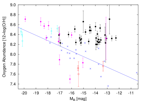
Figure 3: Metallicity-luminosity relation for different types of objects: local isolated dwarf galaxies (crosses), knots in the tidal features (filled/open squares), main group members (filled circles), background objects (open circles).

The metallicity-luminosity relation for the objects in our sample and for isolated dwarf galaxies is shown in Fig. 3. Nearby dwarf irregular galaxies (Richer & McCall 1995) follow the well-known correlation indicated by the linear fit. The massive galaxies in our sample – main galaxies and background objects – also follow this relation. On the other hand, knots along the tidal features deviate significantly from the relation and seem to have a metallicity which is independent of luminosity. The bulk of the emission-line knots in our sample have $12+\log(\mathrm{O}/\mathrm{H})$ in the range $8.3\dots 8.7$ (mean $12+\log(\mathrm{O}/\mathrm{H})$ $=8.34\pm 0.14\approx 1/4\,\sun$) and luminosities $M_{B}=-12\dots-17$ mag. They occupy the position of previously published TDGs (see e.g. Duc et al. 2000). Three objects, AM 0529-565 D, AM 1237-364 g, and AM 1054-325 i, however, have oxygen abundances at least 0.4 dex lower than the rest of the knots.

3.2 Internal extinction

In knots where we could determine internal extinction from the Balmer decrement in addition to the Galactic absorption, we derive $A_{V}$ in the range $0.0\dots 3.3$ mag with a mean of $A_{V}=0.81$ mag.

This is roughly half the mean extinction and range observed in H ii regions in spiral galaxies (e.g. mean $A_{V}=3.1$ mag and $0<A_{V}<6$ mag for H ii regions in the central part of M51, Scoville et al. 2001). This is understandable as our slits sample a much larger field (typically several hundreds of parsecs, see Sect. 4.1.1) than the spatially resolved HST imaging studies of Scoville et al. (typically a few parsecs). Our slits therefore average over several individual H ii regions and the regions between them. As the extinction is typically much higher within H ii regions where the dust accompanies the star formation process, this naturally explains the smaller range and smaller mean value we see in our sample.

Our mean extinction is also comparable to the typical $A_{V}\simeq 1.0$ mag of the young star clusters in the less obscured regions of the Antennae (Whitmore et al. 1999).

3.3 H$\alpha$ luminosities

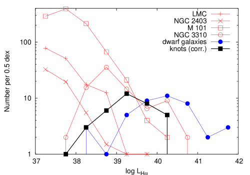
Figure 4: H$\alpha$ luminosity distribution of the observed knots with confirmed higher metallicity compared with literature values for individual H ii regions in spiral disks and total blue dwarf galaxies.

Other authors before have used the H$\alpha$ luminosity to discriminate between candidates for TDGs and normal H ii regions (see e.g. Iglesias-Páramo & Vílchez 2001). We have compiled the H$\alpha$ luminosities of all the tidal knots studied in this survey. Note that the raw luminosities (as e.g. presented in Table 3) are lower limits since they are measured with an aperture-limited slit and not from narrow band imaging. From the size of the optical knots as measured on $B$-band images and the area covered by the slit, we have derived correction factors between 1.5 and 5 depending on the coverage of the knot by the slit and used these to estimate the total H$\alpha$ luminosities of the knots. The average H$\alpha$ luminosity we derive is $2.2\cdot 10^{39}$ erg s^-1. How does this value compare with that measured in typical H ii regions of disk galaxies and other dwarf galaxies?

A histogram of the H$\alpha$ luminosity distribution of the tidal knots is shown in Fig. 4 where it is compared to the luminosity function (LF) of H ii regions in four nearby galaxies of various morphological types (the LMC, NGC 2403, M 101, and NGC 3310). The data was extracted from the catalog of Kennicutt et al. (1989), compiled from ground-based narrow band images. This plot shows an apparent large diversity in the shapes of the H ii LFs. All individual H ii regions in the LMC and the Sc spiral NGC 2403 have H$\alpha$ luminosities about one order of magnitude below the most luminous knots in our survey ($\sim 10^{40}$ erg s^-1). The spiral M 101 hosts a few giant H ii regions reaching this value. The LF of the more distant galaxy NGC 3310 (D$\simeq$19 Mpc) is affected by incompleteness for $\log$$L_{\mathrm{H}\alpha}$ $<38.5$ and has a high number of luminous H ii regions with a distribution very similar to that of our knots. This galaxy is very perturbed and probably has recently undergone a merger.

In the same Figure we also present a comparison with the global H$\alpha$ luminosity distribution of “normal” dwarf galaxies consisting of 11 Im and 7 dI galaxies of Gallagher et al. (1989), 12 nearby “amorphous” dwarf galaxies of Marlowe et al. (1997), and 12 blue compact dwarfs of Cairós et al. (2001). The knots have a distribution similar to the low luminosity end of the normal dwarfs, while there are several dwarf galaxies with luminosities one order of magnitude higher than any of the knots in the tidal tails.

3.4 Kinematics

Table 4: Observed velocity gradients

TDG candidate	$\Delta V_{\mathrm{max}}$	$R$	Angle	Extent
	[km s-1]	[kpc]	[°]	(seeing)
AM 0537-292a	70$\dots$360$\pm$50	8.10	43	1$\aas@@fstack{\prime\prime}$5/2$\aas@@fstack{\prime\prime}$7 (1$\aas@@fstack{\prime\prime}$04)
AM 0537-292g	160$\pm$50	12.60	83	2$\aas@@fstack{\prime\prime}$9 (1$\aas@@fstack{\prime\prime}$26)
AM 0547-244a	77$\pm$61	23.60	5	3$\aas@@fstack{\prime\prime}$5 (1$\aas@@fstack{\prime\prime}$00)
AM 0547-244b	220$\dots$485$\pm$80	30.90	85	2$\aas@@fstack{\prime\prime}$4/4$\aas@@fstack{\prime\prime}$4 (1$\aas@@fstack{\prime\prime}$00)
AM 1054-325h	130$\dots$420$\pm$45	6.40	2	2$\aas@@fstack{\prime\prime}$0/3$\aas@@fstack{\prime\prime}$5 (1$\aas@@fstack{\prime\prime}$00)
AM 1159-530a	440$\pm$45	29.30	29	5$\aas@@fstack{\prime\prime}$5 (1$\aas@@fstack{\prime\prime}$04)
AM 1353-272a∗	343$\pm$17	39.30	0	3$\aas@@fstack{\prime\prime}$0 (1$\aas@@fstack{\prime\prime}$02)
AM 1353-272b∗	87$\pm$18	33.70	0	2$\aas@@fstack{\prime\prime}$6 (1$\aas@@fstack{\prime\prime}$02)
AM 1353-272c∗	34$\pm$14	31.60	0	3$\aas@@fstack{\prime\prime}$2 (1$\aas@@fstack{\prime\prime}$02)
AM 1353-272d∗	93$\pm$ 9	28.10	0	4$\aas@@fstack{\prime\prime}$6 (1$\aas@@fstack{\prime\prime}$02)
AM 1353-272k∗	50$\pm$ 7	22.30	0	2$\aas@@fstack{\prime\prime}$2 (1$\aas@@fstack{\prime\prime}$02)
AM 1353-272l∗	24$\pm$ 6	24.70	0	2$\aas@@fstack{\prime\prime}$6 (1$\aas@@fstack{\prime\prime}$02)
AM 1353-272m∗	43$\pm$ 8	28.30	0	3$\aas@@fstack{\prime\prime}$4 (1$\aas@@fstack{\prime\prime}$02)

^∗observed with FORS2 at the VLT (Weilbacher et al. 2002)

Figure 5: Maximum velocity difference $\Delta V_{\mathrm{max}}$ vs. absolute blue magnitude of our TDGs. Filled squares mark TDGs with only one possible $\Delta V_{\mathrm{max}}$, the three cases with two possible values of $\Delta V_{\mathrm{max}}$ have been plotted as 2 connected open squares to visualize the possible range in $\Delta V_{\mathrm{max}}$.

Figure 6: Maximum velocity difference $\Delta V_{\mathrm{max}}$ vs. projected distance nucleus-knot along the tail. Symbols as in Fig. 7.

Figure 7: Maximum velocity difference $\Delta V_{\mathrm{max}}$ vs. angle slit-tail. Symbols as in Fig. 7.

Due to observational constraints, we could only partially sample the velocity curves along the tails from our long-slit and MOS spectra. A striking result from this study is the presence of kinematical structures with large apparent velocity gradients along the tidal tails.

In our low resolution data, we find several instances of knots with discrepant velocities. In a few cases, we have enough spatial resolution to measure apparent velocity gradients at the location of optically detected objects: in AM 0537-292 (Fig. 10), AM 0547-244 (Fig. 11), AM 1054-325 (Fig. 15), and AM 1159-530 (Fig. 16). The apparent velocity differences $\Delta V_{\mathrm{max}}$ between two close regions can be as high as several hundred  km s^-1. In three knots (AM 0537-292a, AM 0547-244b, and AM 1054-325h) we observe substructure even with our low spatial resolution. In these cases, we note the total amplitude of the gradient and $\Delta V_{\mathrm{max}}$ within the brighter knot.
All observed velocity gradients are summarized in Table 4. There, we also list the distance $R$ between the knot in the tidal tail and the nucleus of the parent galaxy along the tail. We also give the angle between the orientation of the slit and the central ridge of the tail, and the extent of the observed velocity gradient.

In Figs. 7 to 7, parameters which might affect the strength of the velocity gradient given by the $\Delta V_{\mathrm{max}}$ variable are plotted. Fig. 7 shows the maximum velocity difference versus the absolute blue magnitude. We do not observe any obvious trend between the stellar mass very – roughly represented by the blue luminosity – and the dynamical mass to which $\Delta V_{\mathrm{max}}$ is presumably a rough indicator. In Fig. 7, we see that $\Delta V_{\mathrm{max}}$ of the knots does not depend on the distance to the nucleus of the parent galaxy: small gradients occur both near to and far away from the parent nucleus. In Fig. 7, we investigate if the angle between the slit and the tail has a significant contribution to the value of the velocity gradient. As the observations of AM 1353-272 with its 7 knots were performed with slits along the tails (Weilbacher et al. 2002), we have a strong selection effect towards low angles, and cannot derive a dependence between the angle and $\Delta V_{\mathrm{max}}$. However, we note that velocity gradients are observed at all angles between the slit and the tail. That means that we see velocity components both along and perpendicularly to the tail.

4 Discussion

The tidal knots we observed appear to have rather unusual characteristics: in particular their large H$\alpha$ luminosities, and the kinematics of their ionized gas, with velocity amplitudes greater than 100 km s^-1 are striking. With such properties, the TDG candidates in our sample appear to be closer to individual dwarf galaxies than to the giant HII regions of spiral disks.

4.1 TDG candidates: between giant HII regions and individual dwarfs galaxies?

4.1.1 H$\alpha$ luminosities

What can we learn from the comparison with the H ii region luminosities? The spatial coverage of our slits is typically 3$\aas@@fstack{\prime\prime}$5$\times$1$\aas@@fstack{\prime\prime}$7 (the extraction width times the slit width for MOS). For the nearby systems ($D\sim 50$ Mpc) we therefore summed the H$\alpha$ flux over a region of 850$\times$410 pc²; for a distance of 150 Mpc this would increase to 2.5$\times$1.2 kpc². From this rough estimate is seems clear that we do not observe individual H ii regions, but cover a region much larger in size. With the value found for M 101 by Pleuss et al. (2000) a minimum distance between H ii regions is 60 pc; then about 100 individual H ii regions would “fit” into the region we sample for our nearby systems and 1000 for the distant ones. With a typical individual luminosity of $10^{37}$ erg s^-1 (Scoville et al. 2001), one would then expect integrated luminosities of $10^{39}\dots 10^{40}$ erg s^-1, similar to the upper end of the luminosity distribution of the knots. The luminous end of our knots will then be the real starbursts in our sample, while the faint end are regions forming stars at a lower level.

The comparison with the sample of dwarf galaxies is more difficult, because several of the objects shown in Fig. 4 are not classical dwarf galaxies with $M_{B}<-17$ mag but have higher blue luminosities. The H$\alpha$ luminosity does not linearly depend on the star formation rate for dwarf galaxies, but is strongly affected by evolutionary effects as shown by Weilbacher & Fritze-von Alvensleben (2001). This does not allow us to draw any conclusions about the star formation rates of both types of objects. In summary, the H$\alpha$ luminosities emitted by the tidal knots appear to be lower than the global $L_{\mathrm{H}\alpha}$ of normal galaxies with $M_{B}\leq-19$ mag. However, they are at least similar to and in most cases exceed those measured in H ii regions located in the disks of nearby spiral galaxies. It seems clear that the knots we observe are actually a conglomerate of several individual H ii regions. If that is the case, one may wonder whether they do belong to a single dynamical object.

4.1.2 Metallicities

Currently known TDGs have metallicities around 1/3 solar (Duc et al. 2000), significantly higher than normal dwarf galaxies of similar luminosity. This can be understood if TDGs are made out of material which was already metal-enriched prior to the current starburst in the progenitor galaxy: they were dynamically built from the outer disks of their parent galaxies where the metallicity is close to this value (Zaritsky et al. 1994). Gas with very low metal abundance exists in the outermost regions of spirals (Ferguson et al. 1998). However, the analysis carried out in Paper I shows that our TDG candidates are likely to contain a significant amount of old stars. Those had to be pulled out from regions in the parent stellar disk which were rather dense and could not be situated far beyond the optical radius. At their location, the metallicity should have been close to that measured in the tidal knots, i.e. 1/4 to 1/3 solar.

Some dynamical simulations (e.g. Barnes & Hernquist 1998) show that the material of the inner and outer parts of a tidal tail came from smaller and larger radii of the progenitor disk, respectively. Due to the observed metallicity gradients of spiral disks, one might expect to see abundance gradients along tidal tails. In the systems AM 0537-292 and AM 1353-272, where we could observe several knots along the tails, however, we do not observe any systematic radial trend in their abundances. All the knots have nearly the same oxygen abundance around $12+\log(\mathrm{O}/\mathrm{H})$ $\approx$8.34. This hints at a process which mixes material from different regions in the progenitor galaxy and has to be checked with new dynamical models.

The three objects with low metal abundances mentioned in Sect. 3.1 also seem to contain a strong old stellar component (Weilbacher et al. 2000). They are therefore most likely pre-existent companion galaxies, which are either projected onto the tidal features or falling into the interacting system.

4.2 Velocity gradients

What do the apparent velocity gradients tell us about the kinematics of the knots? Clearly such amplitudes are not normally observed in the H ii regions of spirals where, after correction for the overall velocity field, only 15 km s^-1 of residual vertical dispersion is observed (Jiménez-Vicente & Battaner 2000). What is then the origin of such “gradients” in our objects? In fact, several different causes are possible.

4.2.1 Projection effects

Most of the velocity gradients that we observe in the knots have an extent of 2 to 4″, i.e. only a few times the FWHM of the typical seeing (see column 2 of Table 4). The lack of spatial resolution and related “smoothing” will cause physically disconnected regions with distinct velocities to appear as being part of a single kinematical entity. Were that the case, the observed velocity gradient would only be apparent and would hide projection effects. Some knots could in fact be external material seen in projection onto the tail. One may also have the cases where several knots of a bent tail or from even different tails project onto each other.

In Sect. 3.4 we noted three cases with two emission line regions within one apparent knot. Although we cannot confirm these instances as projection effects, these are candidates for this type of velocity gradient caused by projection.

4.2.2 Streaming motions along the tails

The overall velocity field of tidal tails is governed by streaming motions resulting from the gravitational tidal forces exerted during the collision. Identifying in them kinematically decoupled entities is difficult when, as in our sample, the global velocity field is only measured at discrete positions. An upper limit to the contribution from streaming motions can be obtained measuring the difference between the central velocity of the tidal knot and the systemic velocity of the parent galaxy. Generally, this velocity offset is much smaller than the small scale velocity gradient found in the tidal objects.

4.2.3 Outflows associated with super-winds

Outflows are known to accelerate gas to high velocities. Superwinds driven outflows seem to prevail in local starbursts (Heckman et al. 1990), in distant Lyman Break Galaxies (Pettini et al. 2001), and in dwarf galaxies (Martin 1998; Bomans et al. 2001). The kinematic signature of such winds are broad or double-peaked emission lines. They are due to the shell-like structures generated by stellar winds, which always show velocity components towards and away from the observer. If part of the shell was shielded from view by dust, it could also produce velocity gradients. We did not find any obvious broadening of the emission lines in regions characterized by a large velocity gradient and only a moderate extinction was measured there, which makes the dust obscuration of one component quite unlikely.

4.2.4 Gravitationally dominated motion

The last possible origin of the velocity gradients is gravitationally dominated motion within an entity that became kinematically independent from its host tail. Some of the $\Delta V_{\mathrm{max}}$ values measured are certainly too large to be caused by true Keplerian rotation of a virialized entity. If the knots were virially relaxed then one would derive a mass of $10^{10}\,M_{\odot}$ for an observed gradient of $\Delta V_{\mathrm{max}}$$=200$ km s^-1 over 1 kpc from the virial theorem. In those cases it is possible that part of the velocity is due to motion of the H ii regions towards the center of an entity in formation. The mass derived using the Virial Theorem would then strongly overestimate the real mass of the knot.

As the blue luminosity typically rises with mass, the velocity gradients are expected to increase with absolute magnitude, if they were all caused by the rotation of massive objects. This is not obvious in Fig. 7: we see high velocity gradients for both faint and bright knots. However, as most of the knots are still inside the tidal tail, show internal structure, and are not relaxed objects, we cannot assume Keplerian rotation. Also, all objects where we could measure velocity gradients are objects with strong emission lines, probably sites of strong star formation, where $M_{B}$ or in general optical luminosities are not a good measure for the mass of the knots. We will further pursue this question using near infrared luminosities in a future paper (Weilbacher et al., in prep.). We also see from Fig. 7 that the number of knots with visible gradients is higher in the outer regions (20 to 35 kpc) than in the inner regions ($<$20 kpc) of our interacting systems. A reason for this could be that decoupled kinematics or bound knots are more difficult to produce in the denser parts of the inner tidal tails.

A good example of a self-gravitating object seems to be AM 1159-530a: the velocity gradient extends over 5$\aas@@fstack{\prime\prime}$5 or 1.6 kpc with two bright H ii regions at both ends. The gradient is confirmed by the detection of absorption lines between the H ii regions with intermediate velocity. Another fainter H ii region further westward has a discrepant velocity and seems to be projected onto this entity or falling into it.

4.2.5 Limitations of these observations

Clearly the large velocity gradients observed with EFOSC2 in a number of interacting systems should be confirmed with observations at higher spectral resolution. To unquestionably prove the amplitude of the gradients, velocity resolutions better than 200 km s^-1 will be required. The system AM 1353-272 in our sample has actually been re-observed with FORS2 on the VLT at a higher spectral resolution confirming velocity gradients in several knots along both tidal tails of the interacting system, with velocity amplitudes in the range $24<$$\Delta V_{\mathrm{max}}$$<343$ km s^-1 (Weilbacher et al. 2002). To overcome the poor sampling of the gradients, imaging with higher spatial resolution is also needed. H$\alpha$ observations with the Fabry-Perot technique (see e.g. Mendes de Oliveira et al. 2001) in some interacting systems are in progress (Duc et al. 2002, in prep.).

4.3 Selecting Tidal Dwarf Galaxies

Are any of the knots present in the interacting systems studied here the progenitors of TDGs? We describe below the steps required to identify a genuine TDG according to the definition cited in Sect. 1 and check whether the objects in our sample fulfill them. A necessary first step is to select the brightest knots in the tidal tails with luminosities of dwarf galaxies ($-10.5\lesssim{}M_{B}\lesssim-17.0$ mag, from Paper I). Together with the new objects presented in Table 5 we start with 44 TDG candidates (including AM 0529-565D).

4.3.1 Redshift criterion

The selection method from Paper I to disentangle star-forming knots along tidal features from background sources using images in three optical broad band filters in combination with evolutionary synthesis modeling is an efficient method (Sect. 2.2). Nevertheless, it is important to check the association with the main interacting system by measuring the spectroscopic redshift of the candidates. This leaves 29 candidates.

4.3.2 Metallicity criterion

Low-mass companion galaxies, existing prior to the collision, can be discriminated from TDG candidates from their low metallicities. While the tidal knots in our sample have almost constant metallicities around $12+\log(\mathrm{O}/\mathrm{H})$ $\approx 8.3$, three objects close to the tidal features have abundances at least 0.4 dex lower than the tidal knot with the lowest abundance. This is puts them close to the luminosity-metallicity relationship of normal dwarf galaxies. A tidal origin can therefore be excluded for these three exceptions. 26 candidates for TDGs are left.

4.3.3 Dynamical criterion

Genuine TDGs should be gravitationally bound. We do not find classical rotation curves or typical velocity dispersion in any of our TDG candidates. Instead, we find several cases of apparent velocity gradients in the knots in the tidal tails. While we cannot yet exclude all other possible causes 13 TDG candidates seem to have kinematics decoupled from the hosting tail. Further data with high resolution will be necessary to prove these gradients as internal kinematics of the individual candidates.

4.3.4 Final sample of TDG candidates

The 13 objects identified as good TDG candidates represent 46% of the knots that were observed spectroscopically and half of the knots left after selecting the knots depending on their metallicity. Note that – given the low resolution of our spectroscopic data – they cannot yet be considered as real TDGs.

From our 14 interacting galaxies 5 (i.e. about 1/3 of the sample systems) have TDG candidates with kinematical signatures. Of those systems, one (AM 1054-325) has only one TDG candidate, which has an optical appearance very similar to other knots in the same system for which we did not detect decoupled kinematics. The other system with only one TDG, AM 1159-530, has one tail with relatively high and one with very low surface brightness. The massive TDG is positioned at the end of the bright tail. In both galaxies with two TDGs (AM 0537-292 and AM 0547-272), they are positioned in the tails on opposite sides of the nucleus. The system AM 1353-272 contains more that half of the TDG candidates we have finally selected, distributed over both tails.

5 Conclusions

We have analyzed a sample of 14 southern interacting galaxies using deep, low resolution spectrophotometry. The knots in the tidal features were previously identified as good TDG candidates by comparing optical broad band imaging with evolutionary synthesis models. The spectra were first used to investigate the association with the interacting system by comparing the redshifts. All knots that were detected are actually associated with the parent galaxies. This shows that our photometric method is a powerful tool for preselecting TDGs. The few knots which were not detected in our spectra could be of a different nature.

We determined the oxygen abundances of the knots and found a mean value of $12+\log(\mathrm{O}/\mathrm{H})$ $=8.34$ with a scatter of $\pm$0.2 dex. Both the mean value and the scatter are in good agreement with those found in the outer disks of spiral galaxies, which precludes the possibility that these knots could be pre-existing objects infalling onto the interacting systems from outside. Three dwarf galaxies close to the tidal features are unlikely to be TDGs due to their low metallicity.

As predicted by our photometric models, the knots are actively forming stars, and some knots may even be starbursts with high H$\alpha$ luminosities. $L_{\mathrm{H}\alpha}$ of the knots within our spectroscopic slits is higher by two orders of magnitude than that of typical individual H ii regions in spiral disks and lower than that of local star-forming galaxies by a factor of 10. However, the flux represents many individual H ii regions whose number depends on the slit width and the distance of the interacting system. Due to the overlap of the distribution of $L_{\mathrm{H}\alpha}$ with “normal” giant H ii regions in spiral disks and the difference to dwarf galaxy luminosities, $L_{\mathrm{H}\alpha}$ is not a good criterion to discriminate TDGs from other phenomena.

We see surprisingly strong velocity differences in some interacting galaxies, and 13 TDG candidates show kinematic signatures which could be internal velocity gradients in these knots. The velocity amplitudes are in some cases more than one order of magnitude higher than those observed in spiral disks. Our analysis and interpretation is hampered by the small angular size of these gradients, which are barely resolved in $\sim$1″ seeing, so we could not discriminate possible decoupled kinematics from other phenomena like chance alignment of multiple bodies which mimic velocity gradients. We can only prove the existence of one strong velocity gradient within the TDG AM 1159-530a, where we see the gradient extending over 5$\aas@@fstack{\prime\prime}$5, which is likely due to the gravitational forces within the body of the TDG. To confirm the velocity gradients of the knots in the tidal tails as decoupled kinematics governed by internal gravitation an improvement of at least a factor two in spatial resolution is required. Higher velocity resolution (better than 200 km s^-1) would be desirable to confirm the amplitude of the velocity gradients. The discussion of both emission line luminosities and velocity gradients is restricted by the nature of our multi-slit spectroscopic data, which allows us to analyze only discrete parts of the whole interacting system. Narrow band imaging would be required to confirm and interpret the full range of H$\alpha$ luminosities found in the TDG candidates. Furthermore, observational methods like Fabry-Perot- or integral field spectroscopy would be required to fully analyze the velocity distributions of the ionized gas in the interacting galaxies and the TDG candidates.

Finally, the data collected in this paper will help us refine our spectrophotometric evolutionary synthesis models for analyzing the starburst properties of the TDG candidates and to derive more accurate predictions of their future evolution.