High Energy Neutrinos from Magnetars

Abstract

Magnetars can accelerate cosmic rays to high energies through the unipolar effect, and are also copious soft photon emitters. We show that young, fast-rotating magnetars whose spin and magnetic moment point in opposite directions emit high energy neutrinos from their polar caps through photomeson interactions. We identify a neutrino cut-off band in the magnetar period-magnetic field strength phase diagram, corresponding to the photomeson interaction threshold. Within uncertainties, we point out four possible neutrino emission candidates among the currently known magnetars, the brightest of which may be detectable for a chance on-beam alignment. Young magnetars in the universe would also contribute to a weak diffuse neutrino background, whose detectability is marginal, depending on the typical neutrino energy.

1. Introduction

The most widely discussed high energy neutrino sources include gamma-ray bursts (e.g. Waxman & Bahcall 1997, 2000; Dai & Lu 2001; Mészáros & Waxman 2001; Guetta, Spada & Waxman 2001), blazars (e.g. Stecker et al. 1991; Atoyan & Dermer 2001) and micro-quasars (e.g. Levinson & Waxman 2001). Another type of objects, pulsars, have been also considered for some time to be high energy neutrino emitters (e.g. Eichler 1978; Helfand 1979). The direct motivation is that pulsars are unipolar generators which induce a large potential to accelerate protons to high energies (see Blasi, Epstein & Olinto 2000; Arons 2003, for recent discussions on the topic). Such high energy protons, when colliding with target photons or materials, can generate neutrinos mainly through pion decay. In the immediate environment of a pulsar (e.g. within its magnetosphere), however, the main difficulty is the lack of a large enough target column density for pion production. The pulsar neutrino emission is therefore usually discussed within the context of pulsar wind nebulae (Beall & Bednarek 2002; Bednarek 2001) or binary systems (e.g. Eichler 1978).

Here we show that the conditions for neutrino production via photomeson interaction are realized in the inner magnetospheres of the so-called “magnetars”, pulsars with superstrong surface magnetic fields ($B_{s}\sim 10^{15}$ G) (Duncan & Thompson 1992; Paczýnski 1992; Usov 1992), if they are young enough to allow acceleration of protons above the photomeson threshold. These objects are the leading candidate for explaining the widely observed soft gamma-ray repeaters (SGRs) and anomalous X-ray pulsars (AXPs) (Thompson & Duncan 1995, 1996; see observational reviews by Hurley 2000, Mereghetti 2000, and a theoretical review by Thompson 2000). We will estimate the high energy neutrino flux of these objects, as well as their detectability with currently operating and planned large area neutrino telescopes, such as AMANDA-II, ICECUBE, ANTARES, NESTOR and NEMO. We will also estimate a diffuse high energy neutrino background contributed by all young magnetars in the universe.

2. Basic picture and photomeson threshold

In the original definition of Thompson & Duncan, magnetars are neutron stars powered by decaying magnetic fields (Goldreich & Reisenegger 1992; Thompson & Duncan 1996; Heyl & Kulkarni 1998; Colpi, Geppert & Page 2000). However, since they are rotating neutron stars, a conventional power source, i.e., the spindown energy of the star should also play a noticeable role. Although in the slowly rotating magnetars (corresponding to SGRs and AXPs) the spindown power is much lower than the magnetic power, it can exceed the magnetic power during the magnetar’s early life time when the star spins much more rapidly. In any case, there are in principle two main energy sources that power a magnetar. Within the context of our proposed neutrino production mechanism, the dominant photomeson interaction leading to neutrinos occurs through the $\Delta$-resonance,

$$p\gamma\to\Delta\to n\pi^{+}\to n\nu_{\mu}\mu^{+}\to n\nu_{\mu}e^{+}\nu_{e}\bar{\nu}_{\mu}.$$ (1)

In magnetars, the spindown power serves to accelerate protons, and the magnetic power provides copious near-surface photon targets, so that the condition for photomeson interaction is in principle realized. In order to achieve substantial neutrino production rate, however, a threshold condition

$$\epsilon_{p}\epsilon_{\gamma}\lower 4.0pt\hbox{$\buildrel>\over{\sim}$}0.3~{}({\rm GeV})^{2}f_{g}$$ (2)

has to be satisfied. Here

$$f_{g}\equiv(1-\cos\theta_{p\gamma})^{-1}$$ (3)

is a geometric factor, where $\theta_{p\gamma}$ is the maximum lab-frame incidence angle between protons and photons.

The maximum potential drop of a magnetar with the rotation frequency, $\Omega=2\pi/P$ (where $P$ is the period), and surface magnetic field at the pole, $B_{p}=10^{15}{\rm G}B_{p,15}$, is

$$\Phi=\frac{\Omega^{2}B_{p}R^{3}}{2c^{2}}\simeq 6.6\times 10^{15}~{}{\rm V}~{}B_{p,15}R_{6}^{3}P^{-2}~{},$$ (4)

where $R=10^{6}{\rm cm}R_{6}$ is the stellar radius. For a fraction $f=0.5f_{1/2}$ (the nominal value is for the case assuming a random distribution of the inclination angles) of the magnetars whose spin and magnetic moment point in opposite directions, i.e., ${\bf\Omega}\cdot{\bf B}_{p}<0$, the spin-induced parallel electric field accelerates positive charges from the surface. The neutron star surface composition is poorly known. Current modeling of the X-ray data from some nearby isolated neutron stars suggests that it likely consists of light elements such as hydrogen or helium (Zavlin, Pavlov & Trümper 1998; Sanwal et al. 2002) rather than heavy elements such as iron. Recently, Ibrahim et al. (2002, 2003) reported discoveries of the cyclotron resonance features from SGR 1806-20 during outburst which are well interpreted as proton cyclotron features in a magnetar environment, lending credence that the surface composition of magnetars is hydrogen. Here we assume a hydrogen composition of the magnetar surface. According to the standard pulsar theory, protons are accelerated from the polar cap region within charge-depleted gaps (e.g. Ruderman & Sutherland 1975; Arons & Scharlemann 1979). If surface temperatures of magnetars are high enough to allow free emission of protons, space-charge limited flow models of electron acceleration (Arons & Sharlemann 1979; Harding & Muslimov 1998, 2001, 2002) will apply to the acceleration of protons in this case.

Magnetars are also strong X-ray emitters. During the early epochs of their lives, magnetars emit thermal radiation, thought to be due to decay of the strong magnetic fields. This maintains a high X-ray luminosity (typically $10^{35}-10^{36}{\rm erg~{}s^{-1}}$ as observed in SGRs/AXPs) over a long period of time. The nominal field decay law, $dB_{p}/dt=-bB_{p}^{1+\delta}$, leads to a magnetic field strength time dependence $B_{p}(t)={B_{p,0}}/{[1+t/\tau_{mag}]^{1/\delta}}$ (Colpi et al. 2000), where $B_{p,0}$ is the initial surface field at the pole. Thus the magnetar surface field, and hence its quiescent X-ray luminosity, remains almost constant for a typical decaying timescale $\tau_{mag}=(b\delta B_{p,0}^{\delta})^{-1}\sim 10^{4}$ yr. The observed blackbody temperature for SGR/AXP quiescent emission is $kT_{\infty}\sim(0.4-0.6)$ keV (e.g. Hurley 2000; Meregheti 2001; Thompson 2001). The typical near-surface photon energy is therefore

$$\epsilon_{\gamma}=2.8kT_{\infty}(1+z_{g})\sim(1.6-2.4)~{}{\rm keV},$$ (5)

where $(1+z_{g})\sim 1.4$ is the near-surface gravitational redshift. The threshold proton energy from eq.(2) is therefore

$$\epsilon_{p,th}\sim(125-188)f_{g}~{}{\rm TeV}~{}.$$ (6)

The potential across the polar cap [eq.(4)] drops as $P^{-2}$ as the star spins down. The typical energy of the protons accelerated in the inner gap is a fraction of $e\Phi$, which also drops as the magnetar ages. The proton energy acquired in the inner gap can be written as $\epsilon_{p}=\eta_{p}e\Phi$, where $\eta_{p}$ parameterizes the uncertainties in the utilization of the polar cap unipolar potential. The maximum efficiency could be as high as $\eta_{p,max}\sim(0.15-0.85)$ (eqs.[2] and [7] of Zhang, Harding & Muslimov 2000), if the electric field parallel to the magnetic field line is not effectively screened, and if the particle acceleration is not radiation-reaction-limited. For proton accelerators, radiation reaction is negligible for the known magnetar candidates (SGRs/AXPs), mainly because of the small magnetic field curvature in slow rotators. Soft X-rays could be Lorentz-boosted in the proton’s rest frame and pair-produce in its Coulomb field (Cheng & Ruderman 1977; Heitler 1954), with a cross section $\sigma_{\pm}\sim Z^{2}\alpha\sigma_{T}(3/8\pi)[(28/9)\ln(E^{\prime}_{\gamma}/m_{e}c^{2})-218/27]\sim Z^{2}\cdot 7\times 10^{-27}~{}{\rm cm}^{2}$ for $\epsilon_{p}\sim\epsilon_{p,th}$, where $Z$ is atomic number, $\alpha$ is the fine-structure constant, $\sigma_{T}$ is the Thomson cross section, and $E^{\prime}_{\gamma}$ is the Lorentz-boosted photon energy in the rest frame of the proton. The typical pair-production mean free path is $l_{\pm}\sim(n_{\gamma}\sigma_{\pm})^{-1}\sim 1.3\times 10^{4}$ cm, comparable to that in old normal pulsars whose primary pairs are produced through non-resonant inverse Compton scattering. Comparing with the numerical results in the pulsar case (Harding & Muslimov 2002), the pairs produced in such an environment are likely to be too few to fully screen the parallel electric field before the protons reach the photomeson threshold. The cascade pair multiplicity for old magnetars is small. As a result, $\eta_{p}\sim\eta_{p,max}$ could be achieved in old magnetars, so that

$$\epsilon_{p,max}\simeq\eta_{p,max}e\Phi\simeq(40-220)~{}{\rm TeV}~{}B_{p,15}R_{6}^{3}(P/5~{}{\rm s})^{-2}~{}.$$ (7)

Although in young magnetars the parallel electric fields may be screened before $\epsilon_{p}$ reaching $\epsilon_{p,max}$, this nonetheless happens well above $\epsilon_{p,th}$. Thus, one can define a “neutrino death valley” for magnetars by requiring that $\epsilon_{p,max}$ (7) exceeds the threshold energy $\epsilon_{p,th}$ (6), which gives

$$P<(2.4-6.8)~{}{\rm s}~{}B_{p,15}^{1/2}R_{6}^{3/2}f_{g}^{-1/2}~{}.$$ (8)

The range of periods in the right hand side of eq.(8) defines two diagonal lines in the $P-B_{p}$ plane (Figure 1). Photomeson interactions and neutrino emission cease when the magnetar crosses this valley from left to right during its evolution. Magnetars lying in the valley itself are marginal neutrino emitters, i.e., they could be neutrino-loud for favorable parameters.

3. Discrete sources

Here we investigate the possibility of detecting neutrino emission from the individual known magnetar candidates (i.e. SGRs and AXPs), which are typically slow rotators.

As seen in eq.(8), the location of the neutrino death valley depends on the geometric factor $f_{g}$ (eq.[3]). Below we will discuss the possible value of this factor. For the simplest case, thermal photons are expected to be emitted from the surface semi-isotropically, so that $\theta_{p\gamma}\leq 90^{\rm o}$ and $f_{g}\geq 1$. In recent magnetar models (Thompson, Lyutikov & Kulkarni 2002) the magnetosphere is assumed to be globally twisted and current-carrying. The non-relativistic charges in the closed field line region form a resonant cyclotron screen at a high altitude (about 10 stellar radii) with an optical depth higher than unity (see also Wang et al. 1998 for a similar discussion within the context of normal pulsars). The emergent X-ray photons would endure multiple Comptonization before escaping, and the mechanism is used to interpret the observed hard X-ray non-thermal tail in the SGR/AXP spectrum (Thompson et al. 2002). In such a picture, it is natural to expect some downward X-ray photons (with a luminosity comparable to what is observed) reflected from the resonant cyclotron screen into the open field line region. Here we assume a $\sim 50\%$ efficiency of backscattering of the surface thermal photons, but the real fraction has to be treated more carefully by incorporating the detailed radiation transfer processes. In such a most favorable case, $\theta_{p\gamma}\lower 4.0pt\hbox{$\buildrel<\over{\sim}$}180^{\rm o}$ could be achieved so that $f_{g}\lower 4.0pt\hbox{$\buildrel>\over{\sim}$}1/2$. This is the most optimistic case for neutrino production.

If such a pair reflection screen is ineffective, however, $f_{g}$ is larger. Defining the typical photomeson interaction mean free path as $l_{p\gamma}$ and the physical hot spot radius as $r_{h}$, one can estimate

$$\cos\theta_{p\gamma}=\left\{\begin{array}[]{@{\,}ll}\left[1-\left(\frac{R}{R+l_{p\gamma}}\right)^{2}\right]^{1/2},&l_{p\gamma}\leq l_{cr},\\ \left[1+\left(\frac{r_{h}}{l_{p\gamma}}\right)^{2}\right]^{-1/2},&l_{p\gamma}>l_{cr}.\end{array}\right.$$ (9)

where $l_{cr}$ satisfies the relation $[1+(r_{h}/l_{cr})^{2}][1-(R/R+l_{cr})^{2}=1$, and is the critical height at which the horizon is just the boundary of the hot spot. In typical SGRs/AXPs, the surface area of the hot region is large, which could be roughly estimated as $A\sim L/\sigma[(1+z_{g})T_{\infty}]^{4}\sim 4.0\times 10^{11}~{}{\rm cm}^{2}~{}L_{35}(kT_{\infty}/0.5{\rm keV})^{-4}$, where $\sigma=ac/4$ is the Stefan-Boltzmann constant. This gives a rough estimate of the “hot spot” radius $r_{h}\sim 3.6\times 10^{5}~{}{\rm cm}~{}L_{35}^{1/2}(kT_{\infty}/0.5{\rm keV})^{-2}$. Given a typical neutron star radius $R\sim 10^{6}$ cm and this particular $r_{h}$ value, one can solve for $l_{cr}\sim 3.0\times 10^{5}$ cm. On the other hand, the photomeson interaction mean free path could be estimated as $l_{p\gamma}\simeq(n_{\gamma}\sigma_{p\gamma})^{-1}\simeq 1.8\times 10^{5}~{}{\rm cm}~{}(kT_{\infty}/0.5{\rm keV})^{-3}$, where $n_{\gamma}\sim(a/2.8k)[(1+z_{g})T_{\infty}]^{3}\simeq 1.1\times 10^{22}~{}{\rm cm^{-3}}~{}(kT_{\infty}/0.5{\rm keV})^{3}$ is the soft photon number density, $\sigma_{p\gamma}\sim 5\times 10^{-28}{\rm cm}^{2}$ is the photomeson interaction cross section, and $a$ and $k$ are the blackbody radiation density constant and the Boltzmann constant, respectively. We can see $l_{p\gamma}<l_{cr}$ for typical parameters, so that the first expression in eq.(9) is relevant. The salient feature of this expression is that it does not depend on the poorly determined parameter $r_{h}$, as long as it is large enough. The gravitational bending effect also helps to decrease $f_{g}$. For the above typical parameters, we have $\cos\theta_{p\gamma}=[1-(R/R+l_{p\gamma})^{2}]^{1/2}\sim 0.5$, or $f_{g}\sim 2$. Both $l_{p\gamma}$ and $r_{h}$ are steep function of the surface temperature, but for reasonable magnetar surface temperatures, e.g., $kT_{\infty}>0.4$ keV, $l_{p\gamma}<l_{cr}$ is satisfied. However, $f_{g}$ will be significantly increased for smaller $kT_{\infty}$, rendering all SGRs/AXPs below the neutrino death valley. On the other hand, however, higher surface temperatures (which is usually associated with the post-burst situation) and a larger neutron star radius will decrease $f_{g}$ and significantly ease the threshold condition. Observationally it has been found that the SGR quiescent luminosity is greatly increased for a long period of time (e.g. Woods 2003), so that we expect a more facilitated condition and a higher luminosity for a post-burst magnetar.

In Figure 1, we plot all the SGRs and AXPs with period $P$ and spin-down rate $\dot{P}$ measurements relative to the neutrino death valleys for $f_{g}=1/2$ (dotted), $f_{g}=1$ (solid) and $f_{g}=2$ (dashed). The polar cap magnetic field for each magnetar is estimated as $B_{p}=6.4\times 10^{19}~{}{\rm G}~{}(P\dot{P})^{1/2}R_{6}^{-3}I_{45}^{1/2}$, where $I$ is the stellar moment of inertia. A typical magnetar evolutionary track with $\tau_{mag}\sim 10^{4}$ yr is also plotted, with typical ages marked. We find that, although none of the magnetars are firmly above any of the death valley definitions, four of them are within the $f_{g}\sim 1/2$ valley, two of them are within the $f_{g}=1$ valley, and SGR 1900+14 lies within the $f_{g}=2$ valley.

We estimate the neutrino emission luminosity $L_{\nu}$ for these “marginal” magnetars. If pions decay immediately after production, the neutrino emission power can be estimated as $P_{\nu}\sim 0.05\cdot(4/3)\sigma_{p\gamma}c\gamma_{p}^{2}aT^{4}\sim 4\times 10^{5}{\rm erg~{}s^{-1}}(\epsilon_{p}/100{\rm TeV})^{2}(T_{\infty}/0.5{\rm keV})^{4}$, where the factor $0.05=(1/4)\eta_{p\to\pi}$, $\eta_{p\to\pi}\simeq 0.2$ is the average fraction of the energy transferred from the proton to the pion, and the factor (1/4) takes into account the equal energy distribution among other three leptons besides $\nu_{\mu}$ (Halzen & Hooper 2002). The total number of protons is estimated as $N_{p}\sim n_{gj}\int_{0}^{r_{\nu}}A_{o}(r)dr$, where $n_{gj}=\Omega B(r)/2\pi ce$ is the Goldreich-Julian (1969) number density, $A_{o}(r)$ is the cross section of the open-field line region, and $r_{\nu}\sim R$ is the typical length for effective neutrino radiation. This gives

$$L_{\nu,0} = N_{p}P_{\nu}\sim 2.3\times 10^{33}~{}{\rm erg/s}$$ (10)

$$\times \left(\frac{\eta_{p}}{0.5}\right)^{2}B_{p,15}^{3}R_{6}^{10}\left(\frac{P}{5{\rm s}}\right)^{-6}\left(\frac{T_{\infty}}{0.5{\rm keV}}\right)^{4}.$$

The $\pi^{+}$’s can also undergo radiative loss and possible reacceleration in the unscreened parallel electric field before decaying to $\nu_{\mu}$. The final neutrino luminosity is then

$$L_{\nu}=f_{c}L_{\nu,0},$$ (11)

where $f_{c}$ is a correction factor for cooling or reacceleration. For the four marginal magnetars, reacceleration is not important, since $\epsilon_{p}$ is already close to $\epsilon_{p,max}$. The synchrotron cooling is rapid, and the $\pi^{+}$’s soon settle into their ground Landau state with a parallel energy component $\gamma_{\parallel}=\gamma/(1+(\gamma^{2}-1)\sin^{2}\theta)^{1/2}$ (Zhang & Harding 2000), which is essentially $\sim\gamma$ when the pion injection angle $\theta\sim 0$ (which is usually valid, especially for slow rotators). For threshold interactions, the typical pion Lorentz factor upon production is $\gamma_{\pi^{+}}\sim 2.1\times 10^{5}(\epsilon_{\pi^{+}}/30{\rm TeV})$. The pions cool via inverse Compton scattering (IC) with thermal photons in the Klein-Nishina regime, with a cooling time-scale $\tau_{\rm IC}\sim 3\times 10^{-4}~{}{\rm s}~{}(\epsilon_{\pi^{+}}/30{\rm TeV})^{-1}(\epsilon_{\gamma}/2{\rm keV})^{-4}$, which is shorter than the pion decay time $\tau_{decay}\simeq 2.6\times 10^{-8}~{}{\rm s}~{}\gamma_{\pi^{+}}=5.5\times 10^{-3}~{}{\rm s}~{}(\epsilon_{\pi^{+}}/30~{}{\rm TeV})$. Thus the pions undergo some IC cooling before they decay, and the typical neutrino energy is down by a factor $f_{c}=(0.3/5.5)^{1/2}\sim 0.23$ relative to the $\epsilon_{\nu,th}$. Therefore for discrete sources, the typical neutrino energy is

$$\epsilon_{\nu}\sim 0.05f_{c}\epsilon_{p,th}\sim(1.4-2.2)f_{g}~{}{\rm TeV}.$$ (12)

The final neutrino luminosity is

$$L_{\nu} = L_{\nu,0}f_{c}\sim 5.8\times 10^{32}~{}{\rm erg/s}\left(\frac{\eta_{p}}{0.5}\right)^{2}$$ (13)

$$\times \left(\frac{f_{c}}{0.25}\right)B_{p,15}^{3}R_{6}^{10}\left(\frac{P}{5{\rm s}}\right)^{-6}\left(\frac{T_{\infty}}{0.5{\rm keV}}\right)^{4}.$$

Since the spindown luminosity is $L_{sd}=1.5\times 10^{34}{\rm erg/s}B_{p,15}^{2}R_{6}^{6}(P/5{\rm s})^{-4}$, the neutrino emission efficiency is then

$$\eta_{\nu} = L_{\nu}/L_{sd}\sim 0.04\left(\frac{\eta_{p}}{0.5}\right)^{2}$$ (14)

$$\times \left(\frac{f_{c}}{0.25}\right)B_{p,15}R_{6}^{4}\left(\frac{P}{5{\rm s}}\right)^{-2}\left(\frac{T_{\infty}}{0.5{\rm keV}}\right)^{4}.$$

We assume that this luminosity is beamed into a sweep-averaged solid angle $\Delta\Omega_{\nu}\sim 0.1$, which is typical for a polar cap angle $\sim 0.01$ and a moderate inclination angle of the rotator. A smaller/larger $\Delta\Omega_{\nu}$ increases/decreases the on-beam neutrino flux, but decreases/increases the probability of on-beam detection. For an on-beam observer, the neutrino number flux at earth is

$$\phi_{\nu} = \frac{L_{\nu}}{\Delta\Omega_{\nu}D^{2}\epsilon_{\nu}}\sim 2.1\times 10^{-12}~{}{\rm cm^{-2}~{}s^{-1}}$$ (15)

$$\times \left(\frac{\Delta\Omega_{\nu}}{0.1}\right)^{-1}\left(\frac{\eta_{p}}{0.5}\right)^{2}\left(\frac{f_{c}}{0.25}\right)B_{p,15}^{3}R_{6}^{10}$$

$$\times \left(\frac{P}{{5~{}{\rm s}}}\right)^{-6}\left(\frac{T_{\infty}}{0.5{\rm keV}}\right)^{4}\left(\frac{D}{5~{}{\rm kpc}}\right)^{-2}\left(\frac{\epsilon_{\nu}}{2~{}{\rm TeV}}\right)^{-1},$$

where $D$ is the distance to the source. The probability of detecting a neutrino-induced upward muon with planned neutrino telescopes is $P_{\nu\to\mu}\simeq 1.3\times 10^{-6}(\epsilon_{\nu}/{\rm TeV})$ (Halzen & Hooper 2002), giving an on-beam upward muon event rate

$$\frac{dN}{dAdt}({\rm discrete})\simeq 1.7~{}{\rm km^{-2}yr^{-1}}\left(\frac{\Delta\Omega_{\nu}}{0.1}\right)^{-1}\left(\frac{\eta_{p}}{0.5}\right)^{2}$$

$$\times\left(\frac{f_{c}}{0.25}\right)B_{p,15}^{3}R_{6}^{10}\left(\frac{P}{5~{}{\rm s}}\right)^{-6}\left(\frac{T_{\infty}}{0.5{\rm keV}}\right)^{4}\left(\frac{D}{5~{}{\rm kpc}}\right)^{-2}.$$ (16)

The chances for the observer to be in the neutrino beam are not large. Nonetheless, there is a small but finite probability for directly detecting some neutrinos from these objects. In Table 1, we give the predicted muon event rates for the four magnetar candidates which may be neutrino loud under favorable conditions, assuming an on-beam observation. Since other magnetars all lie below the most favorable $f_{g}=1/2$ death valley, they are definetely below the photomeson threshold, and we do not consider them as neutrino emission candidates. From Table 1, we see that SGR 1900+14 and 1E 1048-5937 may be detected by km³ telescopes with several years of operation, if they are above the photomeson threshold and if their neutrino beams sweep the Earth. Accompanying the neutrinos there should also be electromagnetic signals from $\pi^{0}$-decay and $\pi^{+}$ cooling and cascading. The high $\gamma B$ and $\gamma\gamma$ pair-formation and photon splitting opacity in the strong magnetic fields may degrade the typical photon energy to $\lesssim$ 40 MeV, below the EGRET band (e.g. Harding, Baring & Gonthier 1997; Baring & Harding 2001), but it may fall into the INTEGRAL band.

4. Diffuse flux

A direct inference from the above proposal is that the entire population of young magnetars in the universe will contribute to a diffuse neutrino background, before crossing the neutrino death valley. The number flux of this background can be generally estimated as

$$\bar{\phi}_{\nu}\simeq\frac{0.5f_{1/2}}{4\pi\bar{\epsilon}_{\nu}}\int_{0}^{D_{H}}\left[\int_{0}^{\tau_{mag,\nu}}\frac{L_{\nu}(t)f_{b}(t)}{4\pi f_{b}(t)D^{2}}dt\right]{\cal R}(D)(4\pi D^{2})dD~{},$$ (17)

where $D_{H}\sim 10^{28}$ cm is the Hubble distance, and $\bar{\epsilon}_{\nu}$ is the typical energy of the neutrino background. The inner integral is the average total neutrino energy fluence per magnetar emitted towards earth during its neutrino-loud life time $\tau_{mag,\nu}\sim 5\times 10^{3}$ yr, which is based on the known magnetars being marginal neutrino emitters. Since 9 magnetars have been discovered in the Galaxy with typical ages of $10^{4}$ yr, the local (redshift $z=0$) magnetar birth rate can be conservatively estimated ${\cal R}(0)\simeq 10^{-3}~{}{\rm yr^{-1}galaxy^{-1}}{\cal R}_{-3}\simeq 2\times 10^{-5}~{}{\rm yr^{-1}Mpc^{-3}}{\cal R}_{-3}$, for a number density of galaxies $n_{g}=0.02~{}{\rm Mpc}^{-3}$ (Allen 1973). Assuming that the magnetar birth rate follows the star forming rate, ${\cal R}(z)\simeq{\cal R}(0)(1+z)^{3}$ for $z<2$ (Lilly et al. 1996). The time-dependent beaming parameter $f_{b}(t)$ (which is the fraction of magnetars whose neutrino beams are directed towards us, so the sweep-averaged solid angle of the neutrino beam is $\Delta\Omega(t)=4\pi f_{b}(t)$) cancels out. The outer integral is over the Hubble volume. For remote magnetars, the neutrino flux of an individual source drops as $D^{-2}$ while the total number of magnetars increases as $D^{3}$ for $z\ll 1$. Therefore most of the diffuse neutrino emission comes from the farthest magnetars whose birth rate is the highest.

For young magnetars, the time-dependent neutrino luminosity may be estimated as in §3. There are some noticeable differences, however. For example, due to radiation reaction and possible pair screening effect, $\eta_{p}\ll 1$. On the other hand, the pair screening altitude could be much higher than the altitude where pions are generated, so that pions could undergo substantial reacceleration before decaying. As a result $f_{c}$ could be $\gg 1$. Notice that these uncertainties only influence the typical energy of the neutrino background, $\bar{\epsilon}_{\nu}$, but do not influence the number counts of the neutrino background (17), which can be estimated as follows. The time-dependent neutrino luminosity is $L_{\nu}(t)=A_{pc}(t)cn_{\pi^{+}}(t)\bar{\epsilon}_{\nu}$, where $A_{pc}(t)=\pi\Omega(t)R^{3}/c$ is the time-dependent polar cap area, $\Omega(t)=\Omega_{0}(1+t/t_{c})^{-1/2}$ is the time-dependent spin frequency of the magnetar since birth, and $\Omega_{0}$ and $t_{c}$ are constants dependent on the initial rotation period and polar magnetic field of the magnetar; $n_{\pi^{+}}(t)=\xi n_{{}_{\rm GJ}}(t)=10\xi_{1}n_{{}_{\rm GJ}}(t)$ is the time-dependent number density of pions; $\xi\sim R/l_{p\gamma}\sim 10$ is the typical pion multiplicity; $n_{{}_{\rm GJ}}(t)=\Omega(t)B_{p}/2\pi ce$; $\bar{\epsilon}_{\nu}$ is the typical neutrino energy whose detailed value does not enter the problem (i.e. canceled out in eq.[17]). Averaging over the magnetar neutrino-loud lifetime $\tau_{mag,\nu}$, and properly taking into account the cosmological evolution, we estimate

$$\bar{\phi}_{\nu}\sim 10^{-13}~{}{\rm cm^{-2}s^{-1}sr^{-1}}f_{1/2}\xi_{1}{\cal R}_{-3}.$$ (18)

This background is insensitive to the location of the neutrino death valley ($\propto\ln\tau_{mag,\nu}$), because logrithmically the entire magnetar life-time essentially contribute to the final value equally. The detectability of this background, however, is sensitively dependent on the typical energy of the neutrinos, which in turn depends on whether the secondary pions undergo substantial reacceleration before decaying to neutrinos. This is a difficult problem, which is beyond the scope of the current paper, and may be addressable by performing detailed numerical simulations such as those by Harding & Muslimov (2002). Nonetheless, we can set lower and upper bounds for the typical neutrino energies. If pion reacceleration is unimportant, the typical neutrino energy is bound from below to $\sim 2$ TeV according to the IC cooling argument (§3), in which case the diffuse background is completely masked by the atmospheric background and non-detectable. If pion reacceleration is efficient, however, the typical neutrino energy is bound from above by the radiation reaction limit of the pions, and the typical neutrino energy could reach 1 PeV or even higher. Such a neutrino background would become observationally interesting for ICECUBE if $\bar{\epsilon}_{\nu}\geq 100$ TeV (D. F. Cowen, 2003, private communication), and at such energies, the diffuse emission from other neutrino sources becomes weaker than this component (Protheroe 1999).

5. Discussion

We have argued that young magnetars with oppositely oriented magnetic and spin moments (${\bf\Omega}\cdot{\bf B_{p}}<0$) can emit high energy neutrinos from their polar caps. We point out four neutrino emission candidates (Table 1) among the known magnetars. The chances of detecting neutrinos from these objects with future km³ neutrino telescopes (such as ICECUBE) is small, because their emission is faint and beamed. Nonetheless, it is finite, and we suggest that these are possible discrete neutrino sources for the telescopes to monitor. Furthermore, post-burst magnetars (SGRs) should have higher X-ray luminosities and hence, should contribute higher neutrino fluxes. This enhances the chance of detecting neutrinos from known magnetars. The level of the diffuse neutrino background contributed by young magnetars in the whole universe is weak and marginally detectable, depending on the poorly known typical neutrino energy subject to further detailed modeling.

We have concentrated on the possible photomeson interactions near the magnetar polar cap. However, similar neutrino production processes may also take place in the magnetar wind nebula, which could contribute additional neutrino emission components besides the one discussed here.

Table 1Predicted on-beam neutrino-induced upward muon event rates for the four potential neutrino-emitting magnetars assuming they are above photomeson threshold.

Name	$P({\rm s})$	$\dot{P}(10^{-11}{\rm s/s})$	ref.	$B_{p}(10^{15}{\rm G})$	$D({\rm kpc})$	$\frac{dN}{dAdt}({\rm km^{-2}~{}yr^{-1}})$
SGR 1900+14	5.16	10.9	[1]	1.51	(3.0-9.0)	(1.5-13) (0.1/$\Delta\Omega_{\nu}$)
SGR 0526$-$66	8.04	6.6	[2]	1.47	$\sim$ 50	$\sim$ 0.003 (0.1/$\Delta\Omega_{\nu}$)
1E 1048$-$5937	6.45	2.2	[3]	0.761	(2.5-2.8)	(0.5-0.7) (0.1/$\Delta\Omega_{\nu}$)
SGR 1806$-$20	7.48	2.8	[1]	0.924	(13.0-16.0)	(0.01-0.02) (0.1/$\Delta\Omega_{\nu}$)

Note. — References for the spin parameters. [1] Hurley 2000 and references therein; [2] Kulkarni et al. 2003; [3] Mereghetti 2001 and references therein.

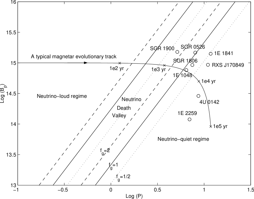
Figure 1.— $P-B_{p}$ diagram of the known magnetars with $P$ and $\dot{P}$ data available (data taken from http://www.atnf.csiro.au/people/pulsar/catalogue, maintained by R. N. Manchester; and Kulkarni et al. 2003 for SGR 0526-66) showing also the neutrino death valley between the two diagonal lines (solid lines for $f_{g}=1$; dotted lines for $f_{g}=1/2$; and dashed lines for $f_{g}=2$, where $f_{g}$ is the angular correction factor for the threshold condition), and a typical magnetar evolutionary track with $\tau_{mag}\sim 10^{4}$ yr (with typical ages marked along the track with crosses).

References

- (1)
- (2) Allen, C. W., 1973, Astrophysical Quantities, The Athlone Press, London & Atlantic Highlands
- (3)
- (4) Arons, J. 2003, ApJ, in press (astro-ph/0208444)
- (5)
- (6) Arons, J. & Scharlemann, E. T. 1979, ApJ, 231, 854
- (7)
- (8) Atoyan, A., & Dermer, C. D. 2001, Phys. Rev. Lett., 87, 221102
- (9)
- (10) Baring, M. G. & Harding, A. K. 2001, ApJ, 547, 929
- (11)
- (12) Beall, J. H., & Bednarek, W. 2002, ApJ, 569, 343
- (13)
- (14) Bednarek, W. 2001, A&A, 378, L49
- (15)
- (16) Blasi, P., Epstein, R. I., & Olinto, A. V. 2000, ApJ, 533, L123
- (17)
- (18) Cheng, A. F. & Ruderman, M. A. 1977, ApJ, 214, 598
- (19)
- (20) Colpi, M., Geppert, U. & Page, D. 2000, ApJ, 529, L29
- (21)
- (22) Dai, Z. G. & Lu, T. 2001, ApJ, 551, 249
- (23)
- (24) Duncan, R. C. & Thompson, C. 1992, ApJ, 392, L9
- (25)
- (26) Eichler, D. 1978, Nature, 275, 725
- (27)
- (28) Goldreich, P. & Julian, W. H. 1969, ApJ, 157, 869
- (29)
- (30) Goldreich, P. & Reisenegger, A. 1992, ApJ, 395, 250
- (31)
- (32) Guetta, D., Spada, M., & Waxman, E. 2001, ApJ, 559, 101
- (33)
- (34) Halzen, F. & Hooper, D. 2002, Rep. Prog. Phys., 65, 1025
- (35)
- (36) Harding, A. K., Baring, M. G. & Gonthier, P. L. 1997, ApJ, 476, 246
- (37)
- (38) Harding, A. K. & Muslimov, A. G. 1998, ApJ, 508, 328
- (39)
- (40) —–. 2001, 556, 987
- (41)
- (42) —–. 2002, 568, 862
- (43)
- (44) Heitler, W. 1954, Quantum Theory of Radiation, (Oxford: Oxford University Press, 1954)
- (45)
- (46) Helfand, D. J. 1979, Nature, 278, 720
- (47)
- (48) Heyl, J. S. & Kulkarni, S. R. 1998, ApJ, 506, 61
- (49)
- (50) Hurley, K. 2000, in Proc. Fifth Compton Symp., Portsmouth, NH, USA, Sep. 1999, AIP Conf. Proc. 510 (eds. M. L. McConnel & J. M. Ryan), 515
- (51)
- (52) Ibrahim, A. I., Safi-Harb, S., Swank, J. H., Parke, W. et al. 2002, ApJ, 574, L51
- (53)
- (54) Ibrahim, A. I., Swank, J. H., & Parke, W. 2003, ApJ, 584, L17
- (55)
- (56) Kaplan, D. L. et al. 2001, ApJ, 556, 399
- (57)
- (58) Kulkarni, S. R. et al. 2003, ApJ, 585, 948
- (59)
- (60) Levinson, A. & Waxman, E. 2001, Phys. Rev. Lett., 87, 171101
- (61)
- (62) Lilly, S. J. et al. 1996, ApJ, 460, L1
- (63)
- (64) Marsden, D., Lingenfelter, R. R., Rothschild, R. E. & Higdon, J. C. 2001, ApJ, 550, 397
- (65)
- (66) Mereghetti, S. 2001, in The neutron star - black hole connection, Proc. of the NATO Advanced Study Institute, Elounda, Crete, Greece, 7-18 June 1999 (eds. C. Kouveliotou, J. Ventura, & E. Van den Heuvel), 351
- (67)
- (68) Mészáros, P., & Waxman, E. 2001, Phys. Rev. Lett., 87, 171102
- (69)
- (70) Paczýnski, B. 1992, AcA, 42, 145
- (71)
- (72) Protheroe, R. J. 1999, Nucl. Phys. B Proc. Supp., 77, 465
- (73)
- (74) Ruderman, M. A. & Sutherland, P. G. 1975, ApJ, 196, 51
- (75)
- (76) Sanwal, D., Pavlov, G. G., Zavlin, V. E. & Teter, M. A. 2002, ApJ, 574, L61
- (77)
- (78) Stecker, F. W., Done, C., Salamon, M. H. & Sommers, P., 1991, Phys. Rev. Lett., 66, 2697
- (79)
- (80) Thompson, C. 2001, in The neutron star - black hole connection, Proc. of the NATO Advanced Study Institute, Elounda, Crete, Greece, 7-18 June 1999 (eds. C. Kouveliotou, J. Ventura, & E. Van den Heuvel), 369
- (81)
- (82) Thompson, C. & Duncan, R. C. 1995, MNRAS, 275, 255
- (83)
- (84) —–. 1996, ApJ, 473, 322
- (85)
- (86) Thompson, C., Lyutikov, M., & Kulkarni, S. R. 2002, ApJ, 574, 332
- (87)
- (88) Usov, V. V. 1992, Nature, 357, 472
- (89)
- (90) Wang, F. Y.-H., Ruderman, M., Halpern, J. P. & Zhu, T. 1998, ApJ, 498, 373
- (91)
- (92) Waxman, E. & Bahcall, J. N. 1997, Phys. Rev. Lett., 78, 2292
- (93)
- (94) —–. 2000, ApJ, 541, 707
- (95)
- (96) Woods, P. M. 2003, to appear in ”High Energy Studies of Supernova Remnants and Neutron Stars” (COSPAR 2002), (astro-ph/0304372)
- (97)
- (98) Zavlin, V. E., Pavlov, G. G. & Trúmper, J. 1998, A&A, 331, 821
- (99)
- (100) Zhang, B., & Harding, A. K. 2000, ApJ, 532, 1150
- (101)
- (102) Zhang, B., Harding, A. K. & Muslimov, A. G. 2000, ApJ, 531, L135
- (103)