Difficulties with Recovering The Masses of Supermassive Black Holes from Stellar Kinematical Data

Abstract

We investigate the ability of three-integral, axisymmetric, orbit-based modeling algorithms to recover the parameters defining the gravitational potential (mass-to-light ratio $\Upsilon$ and black hole mass $M_{\bullet}$) in spheroidal stellar systems using stellar kinematical data. We show that the potential estimation problem is generically under-determined when applied to long-slit kinematical data of the kind used for most black hole mass determinations to date. A range of parameters ($\Upsilon,M_{\bullet}$) can provide equally good fits to the data, making it impossible to assign best-fit values. The indeterminacy arises from the large variety of orbital solutions that are consistent with a given mass model. We demonstrate the indeterminacy using a variety of data sets derived from realistic models as well as published observations of the galaxy M32. The indeterminacy becomes apparent only when a sufficiently large number of distinct orbits are supplied to the modeling algorithm; if too few orbits are used, spurious minima appear in the $\chi^{2}(\Upsilon,M_{\bullet})$ contours, and these minima do not necessarily coincide with the parameters defining the gravitational potential.

We show that the range of degeneracy in $M_{\bullet}$ depends on the degree to which the data resolve the radius of influence $r_{h}$ of the black hole. For ${\rm FWHM}/2r_{h}\gtrsim 0.5$, where FWHM refers to the instrumental resolution, we find that only very weak constraints can be placed on $M_{\bullet}$. In the case of M32, our reanalysis demonstrates that when a large orbit library is used, data published prior to 2000 (${\rm FWHM}/2r_{h}\approx 0.25$) are equally consistent with black hole masses in the range $1.5\times 10^{6}{{\cal M}_{\odot}}<M_{\bullet}<5\times 10^{6}{{\cal M}_{\odot}}$, with no preferred value in that range. Exactly the same data can reproduce previous published results with smaller orbit libraries. While the HST/STIS data for this galaxy (${\rm FWHM}/2r_{h}\approx 0.06$) may overcome the degeneracy in $M_{\bullet}$, HST data for most galaxies do not resolve the black hole’s sphere of influence and in these galaxies the degree of degeneracy allowed by the data may be greater than previously believed.

We investigate the effect of regularization, or smoothness constraints, on the degree of degeneracy of the solutions. Enforcing smoothness reduces the range of acceptable models, but we find no indication that the true potential can be recovered simply by enforcing smoothing. For a given smoothing level, all solutions in the minimum-$\chi^{2}$ valley exhibit similar levels of noise; as the smoothing is increased, there is a systematic shift in the midpoint of the $\chi^{2}$ valley, until at a high level of smoothing the solution is biased with respect to the true solution. These experiments suggest both that the indeterminacy is real – i.e., that it is not an artifact associated with non-smooth solutions – and that there is no obvious way to choose the smoothing parameter to ensure that the correct solution is selected.

1. Introduction

Supermassive black holes (SBHs) are believed to be the central engines of active galactic nuclei and quasars Lynden-Bell (1969). A substantial fraction of the mass involved in the energy production is expected to collapse onto the central black hole. There is now irrefutable dynamical evidence for a SBH at the center of our Galaxy Genzel et al. (1997); Ghez et al. (1998) and in NGC 4258 Miyoshi et al. (1995). In addition there is compelling evidence that compact mass concentrations – probably SBHs – exist in the nuclei of a handful of other galaxies. The STIS GTO program (Joseph et al. (2001); Bower et al. (2001); Merritt et al. 2001), and several HST GO projects Sarzi et al. (2001); Barth et al. (2001); Hughes et al. (2001); Gebhardt et al. (2003) have begun to extend the search for SBHs to a sample of roughly a hundred galaxies.

Before this search was fully underway, a tight empirical correlation was discovered between the masses of SBHs and the velocities of stars in their host bulges. The $M_{\bullet}-\sigma$ relation:

$$M_{\bullet}=(1.48\pm 0.24)\times 10^{8}{{\cal M}_{\odot}}\left({\sigma\over 200{\rm km\ s}^{-1}}\right)^{\alpha},$$ (1)

$$\alpha=4.65\pm 0.48$$

Ferrarese and Merritt (2000); Gebhardt et al. 2000b , relates $M_{\bullet}$ to a measure of the stellar velocity dispersion in a region larger than the region directly influenced by the SBH, $r_{h}\equiv GM_{\bullet}/\sigma^{2}$ (slope and normalization taken from Merritt & Ferrarese 2001b ). The tightness of the relation depends crucially on the sample used to define it: SBHs whose masses were derived from data that resolve $r_{h}$ define a relation with negligible scatter, $\tilde{\chi}^{2}\lesssim 1$, while including all published detections regardless of their quality yields a weaker relation and a different slope Ferrarese and Merritt (2000); Merritt & Ferrarese 2001a ; Merritt & Ferrarese 2001b . Almost all SBH masses derived from ground-based, stellar-kinematical data Magorrian et al. (1998) scatter above the $M_{\bullet}-\sigma$ relation defined by the more secure masses.

If the current normalization of the $M_{\bullet}-\sigma$ relation, equation (1), is correct, SBHs in the more distant of the Magorrian et al. (1998) galaxies are too small for their radii of influence to have been resolved by existing telescopes. Modeling of such data is prone to systematic errors, the sign and magnitude of which depend on the form of the dynamical model fit to the stellar motions and the degree of under-resolution. van der Marel (1999) argued that the two-integral (2I) axisymmetric models used by Magorrian et al. (1998) were likely to give spuriously large values of $M_{\bullet}$.

The discovery that the ground-based mass estimates were systematically high resolved the discrepancies between the mean SBH mass inferred from quasar statistics and reverberation mapping of (mostly) distant galaxies, on the one hand, and from the kinematics of nearby galaxies on the other Richstone et al. (1998). All techniques now yield a mean ratio of SBH mass to bulge mass of $\sim 10^{-3}$ and a mean SBH mass density of $\sim 3\times 10^{5}{{\cal M}_{\odot}}{\rm pc}^{-3}$ Ferrarese (2002); Tremaine et al. (2002).

The biases associated with 2I modeling can in principle be removed if the data are compared with fully general, “three integral” (3I) axisymmetric models, in which any distribution of orbits is allowed . Such models have been used to estimate $M_{\bullet}$ in a number of galaxies (van der Marel et al. (1998); Cretton & van den Bosch (1999); (Emsellem et al. 1999); Gebhardt et al. 2000a ; Gebhardt et al. (2003); Cappellari et al. 2003a ;
Verolme et al. (2002)) . In contrast to 2I models, 3I models can precisely reproduce a given mass distribution with many different orbital populations. This extra freedom is so great that one does not necessarily expect to find a unique potential that yields a best fit to the data; indeed there may exist many choices for the parameters ($\Upsilon,M_{\bullet}$) that reproduce the data equally well. This indeterminacy of potential estimation is well documented Merritt 1993a ; Gerhard et al. (1998).

In this paper, we discuss the importance of the degeneracy in the context of stellar-dynamical estimates of $M_{\bullet}$ in galactic nuclei. We apply a state-of-the-art 3I modeling algorithm to various data sets, including previously-analyzed data from M32, as well as simulated data generated from an axisymmetric model of M32. We investigate how accurately a 3I modeling algorithm can recover the true values of $M_{\bullet}$ and $\Upsilon$, and how sensitively the estimates of those quantities, and their errors, depend on the quality of the data, the character of the data, and the number of orbits included in the model, and the degree of smoothing applied.

Our conclusion is that the indeterminacy problem is often severe. Even when modeling “good” data, the range of values of $M_{\bullet}$ that can reproduce the data equally well is typically very large. (We define “good” data as data that resolve the SBH’s sphere of influence; extend far enough in radius to constrain the global mass-to-light ratio; include high-order moments of the line-of-sight velocity distributions; and have small errors.) This degeneracy can formally be reduced by placing restrictions on the allowed functional form of the stellar distribution function; indeed it was in just this way that Magorrian et al. (1998) achieved their fits, by restricting $f$ to a two-integral form. Another such restriction, common in the more recent studies, is to force the 3I $f$ to be smooth Cretton et al. (1999); Gebhardt et al. (2003); Cappellari et al. 2003a ; Verolme et al. (2002). Smoothness constraints might reasonably be expected to guide the optimization routine away from solutions that vary strongly between the data points, achieving good fits only by virtue of the discrete character of the data Merritt & Fridman (1996); Jalali & de Zeeuw (2002). However we find no indication that smoothness on its own can overcome the inherent degeneracy in the potential estimation problem. Furthermore, if used carelessly, smoothness constraints can bias the solution, yielding an apparent best-fit value for $M_{\bullet}$ which lies far from the true value.

In § 2 we give a detailed description of our 3I modeling algorithm. § 3 reviews the reasons why the potential estimation problem is expected to be under-determined in the axisymmetric geometry. § 4 presents a 2I model of M32 that we use as a test case for our algorithm. § 5 and § 6 present detailed results of fits of simulated data sets derived from the M32 model, and § 7 describes the results of a re-analysis of published data for this galaxy. § 8 describes how the introduction of additional regularization or smoothness constraints affects the results when applied to the simulated M32 data. § 9 is a discussion of the implications of our results for the recovery of $M_{\bullet}$ in nearby galaxies, and § 10 sums up.

2. Modeling Algorithm

2.1. Density and Potential

We construct dynamical models of axisymmetric stellar systems with mass density $\rho(\varpi,z)$ and potential $\Phi(\varpi,z)$; $z=0$ defines the equatorial plane. The mass density may contain contributions from stars, $\rho_{*}$, as well as other components such as dark matter or a central black hole. The contribution to the mass density from the stars is derived from the luminosity density $j_{*}(\varpi,z)$ via the mass-to-light ratio $\Upsilon$, $\rho_{*}(\varpi,z)=\Upsilon j_{*}(\varpi,z)$. In this paper (as in most previous studies), $\Upsilon$ will be considered a constant, although in general, a spatially-dependent $\Upsilon$ could be used to represent the contribution of a dark halo or a radially-varying stellar mass-to-light ratio.

Obtaining $j_{*}$ from the observed surface brightness profile is an under-determined problem for axisymmetric galaxies except when the symmetry axis lies in the plane of the sky Gerhard & Binney (1996); Rybicki (1987); Romanowsky & Kochanek (1997). But galaxies in which the mass is stratified on similar concentric ellipsoids do have unique deprojections provided the inclination angle $i$ is known. In general we would obtain $\rho(\varpi,z)$ via a non-parametric deprojection of the observed surface brightness profile (Merritt & Tremblay 1994, Merritt et al. 1997). In what follows, the focus is on the indeterminacy resulting from incomplete kinematical information and we will assume the freedom to specify a unique functional form for $\rho_{*}(\varpi,z)$.

The gravitational potential is assumed to be of the form

$$\Phi(\varpi,z)=\Phi_{*}(\varpi,z)-GM_{\bullet}/(\sqrt{\varpi^{2}+z^{2}}),$$ (2)

where $\Phi_{*}(\varpi,z)$ is the potential derived from the stellar luminosity profile and the second term is the contribution from a central black hole. An efficient way to evaluate $\Phi_{*}(\varpi,z)$ is via a truncated multipole expansion van Albada & van Gorkom (1977):

$$\Phi_{*}(r,\theta) = -2\pi G\sum_{l=0}^{l_{\rm max}}{P_{l}(\cos\theta)}\times$$

$$\left[{\frac{1}{r^{l+1}}}\int_{0}^{r}{\rho_{l}(a)a^{l+2}{\rm d}a}+r^{l}\int_{r}^{\infty}{\rho_{l}(a){\frac{{\rm d}a}{a^{l-1}}}}\right],$$

Expressions for the forces in cylindrical coordinates are easily derived from equation (2.1). The density distribution is required on a grid in $(r,\theta)$. Since all real elliptical galaxies have moderate to steep central density cusps, the radial grid is chosen to be logarithmically spaced. The potential between grid points is evaluated by bicubic spline interpolation.

It proved convenient to choose an analytic form for the luminosity density. Since the simulated data described below were generated from a 2I model of M32 (see § 3), we adopted the parametrized form of the luminosity density used by van der Marel et al. (1998) (hereafter vdM98) in the construction of this model:

$$j_{*}(\varpi,z)=j_{*}(m)=j_{0}(m/b)^{\alpha}[1+(m/b)^{2}]^{\beta}[1+(m/c)^{2}]^{\gamma},$$ (4)

where $m^{2}=\varpi^{2}+(z/q)^{2}$, and $\alpha=-1.435$, $\beta=-0.423$, $\gamma=-1.298$, $b=0.55$″, $c=102.0$″, $q=0.73(i=90^{\circ})$.

The potential due to the density distribution (4) can be derived directly via Poisson’s equation and the forces via numerical quadrature. We tested the accuracy of the multipole expansion scheme by comparing the force evaluations with those obtained via quadrature. We took $l_{\rm max}=6$ and set the inner radius of the grid at $6\times 10^{-4}$″. 80 radial grid points and 8 polar grid points were selected for the multipole expansion. These tests showed that the multipole expansion gives forces that have fractional errors of $\sim 10^{-3}$ at the innermost radius, dropping rapidly with increasing radius. The use of the multipole expansion scheme results in an approximately eightfold reduction in orbit integration times compared with force evaluation via quadrature.

2.2. The Orbit Library

All orbits in a steady-state axisymmetric Hamiltonian respect at least two isolating integrals of the motion: the orbital energy $E$ and the angular momentum $L_{z}$ about the symmetry axis. A non-resonant orbit with only these two integrals would completely fill the region of the meridional plane enclosed by the zero-velocity curve (ZVC). However numerical studies e.g. Contopoulos (1960); Ollongren (1962); Richstone (1982) show that most orbits also conserve a third integral, $I_{3}$, which confines the orbit to a subset of the allowed meridional-plane region. When the third integral is present, the orbit touches the ZVC at a finite number of points. Launching orbits from uniformly-spaced points on the ZVC ensures a reasonable sampling of the third dimension of phase space accessible to regular orbits.

Each orbit is integrated for a fixed number of periods and its properties stored. The number and nature of stored properties is determined by the available data. Since the purpose of generating the orbit library is to determine the linear combination of orbits that best reproduces the data, we need to “observe” each orbit under conditions as close as possible to the conditions under which the data were taken. This involves convolving the intrinsic orbital properties with the seeing function, as well as averaging over the observed slit width and aperture size. The result is a set of quantities associated with the orbits that can be linearly co-added and compared with the data, without any need for interpolation. In the remainder of this section we describe the various steps in the generation of the orbit library.

2.2.1 Orbital Initial Conditions

Our choice of orbital initial conditions is similar to that of vdM98 and Cretton et al. (1999). We first select a radial grid of $N_{E}$ points logarithmically spaced from $\varpi_{\rm min}$ to $\varpi_{\rm max}$; for the mass model of equation (4), we took $\varpi_{\rm min}=5\times 10^{-4}$ ″and $\varpi_{\rm max}=7.5\times 10^{3}$ ″. At each radial grid point $\varpi_{i}$, the energy of the circular orbit of radius $\varpi_{i}$ is $E_{i}=(1/2\varpi_{i})\partial\Phi/\partial\varpi_{i}+\Phi(\varpi_{i},0)$, thus defining the energy grid. The maximum allowed angular momentum at energy $E_{i}$, $L^{i}_{\rm max}$, is determined by the angular momentum of a circular orbit. At each energy we choose $N_{J}$ regularly-spaced values in $L_{z}$ on the open interval (0, $L^{i}_{\rm max}$) (i.e. excluding $L^{i}_{j}=0$ and $L^{i}_{j}=L^{i}_{\rm max}$, which correspond to radial and circular orbits respectively). This grid only selects orbits with one sense of rotation about the symmetry axis, but orbits with the opposite sense of rotation are trivially obtained by flipping the sign of the velocity. For each pair $(E_{i},L^{i}_{j})$ we then compute the ZVC, the curve on the meridional plane where the effective potential is zero:

$$\Phi_{\rm eff}=\Phi(\varpi,z)+{\frac{1}{2}}{\frac{L_{z}^{2}}{\varpi^{2}}}=0.$$

The third quantity chosen to define an orbit is the angle $\beta$ between the major axis ($x$) and the line joining the origin and a point on the ZVC. We select $N_{\beta}$ equally-spaced angles $\beta$ in the open interval $(0,\pi)$. In the tests described below, we computed for each mass model a library with $(N_{E},N_{L},N_{\beta})=(62,9,8)$ for a total of $\sim 4464$ orbits having one sign of rotation, or $8928$ orbits overall.

Orbits were integrated in the meridional plane using an explicit Runge-Kutta integrator of order 8(5,3) due to (Hairer & Wanner 1993) with adaptive step size control but which give dense output at equally space time intervals. The integration interval ($N_{\rm period}$) was taken to be 200 periods of the circular orbit at each energy and orbits were sampled at $N_{\rm step}=100$ equally-spaced time steps during each orbital period. Orbits were launched from the ZVC with initial velocities $v_{\varpi}=v_{z}=0$. At the end of the integration the energy of the orbit was always conserved to a (relative accuracy) of better than $1\times 10^{-5}$. While integrations were carried out in the meridional plane, we require the orbit in Cartesian coordinates in order to compare with the observed data. Cartesian coordinates $(x,y,z,v_{x},v_{y},v_{z})$ were computed by assuming a random azimuthal angle $0\leq\phi\leq 2\pi$ at each time step and $v_{\phi}(t)=L^{i}_{j}/\varpi(t)$. Unlike other authors e.g. Cretton et al. (1999); Verolme et al. (2002) we do not see the need to “dither” the orbits to create packets of orbits. Also, unlike these authors we compute the forces precisely (from the multipole expansion routine) at each point in the orbit rather than interpolating from forces stored on a grid in $(\varpi,z)$. Once the orbit is integrated in the potential the observed properties of the orbit need to be transformed to the correct viewing angle based on the assumed inclination $i$ of the model; this gives an additional set of coordinates $(x^{\prime},y^{\prime},z^{\prime},v^{\prime}_{x},v^{\prime}_{y},v^{\prime}_{z})$, with $x^{\prime}$ and $z^{\prime}$ coinciding with the projected major and minor axes respectively and $v^{\prime}_{y}$, the observed line-of-sight velocity.

2.2.2 The Storage Grids

The orbital properties are stored on three kinds of grid, depending on the type of observational constraint. These storage grids are similar to those used by other authors Rix et al. (1997); van der Marel et al. (1998); Cretton et al. (1999); Verolme et al. (2002).

To reproduce the known mass distribution of the model (self-consistency constraints), we store the orbital contribution to the mass of each cell on a grid in the $(r,\theta)$-plane. We use 20 logarithmically-spaced radial bins and 16 equally-spaced bins in $\theta$ ($0\leq\theta\leq\pi/2$). For the M32 mass model described above, the lower and upper radial grid points were at $\sim 5\times 10^{-4}$″and 102″. At each time step the orbital position ($\varpi$, $|z|$) determines the cell to which a fractional weight $\delta$ is added. The total mass contributed by the $\alpha$th orbit to the grid cell centered on $(r,\theta)$ is a sum of all the fractional weights and is represented by $m^{\alpha}_{r\theta}$.

The orbital kinematics are stored on 3-D grids in the projected coordinates $(x^{\prime},z^{\prime},v^{\prime}_{y})$. Each set of observations (defined by different seeing, aperture locations etc.) requires a separate grid. The grids themselves are square in the $x^{\prime}-z^{\prime}$-plane with outer boundaries set by the outermost observed aperture. For the models in this paper the typical grid consisted of $267\times 267$ pixels with the bin width equal to $\sim 1/8$ the FWHM of the PSF (or seeing in the case of ground based data). So for instance for all data from the HST (FOS and STIS) the orbit libraries were stored on grids with pixel width 0.0125″ whereas for ground based CFHT data (e.g. Bender et al. 1996) the pixel width was 0.038″. The grid in the velocity dimension has 107 points in the range [-800km s^-1 , 800km s^-1  ] or a velocity sampling of 15.1km s^-1 . This is smaller than the velocity scale of the STIS spectrograph ($\sim$ 19km s^-1   per pixel at $\sim 8500$ Å  or a wavelength scale of 0.56 Å  per pixel). In general it was found necessary to use a velocity range which is at least $\pm 4-6\times\sigma_{\rm max}$, where $\sigma_{\rm max}$ is the largest observed velocity dispersion.

It is standard practice to generate orbit libraries for a single value of the mass-to-light ratio $\Upsilon_{0}$ and to generate libraries for all other $\Upsilon$ values by scaling the velocities by a factor $\sqrt{\Upsilon/\Upsilon_{0}}$ (e.g. vdM98; Cretton et al. 1999). We will refer to the library generated using $M/L=\Upsilon_{0}$ as the “primary library” for each value of $M_{\bullet}$. It is important that the choice of $\Upsilon_{0}$ be determined by a prior estimate of the best-fit value of $M/L$ (based on e.g. 2I or spherical models). If the velocities in the primary library are stored on a grid with range $[-v_{0},v_{0}]$ and grid spacing $\delta v_{0}$, the scaled velocities for any other $\Upsilon$ will have a range $[-\sqrt{\Upsilon/\Upsilon_{0}}v_{0},\sqrt{\Upsilon/\Upsilon_{0}}v_{0}]$ and velocity spacing of $\sqrt{\Upsilon/\Upsilon_{0}}\delta v_{0}$. The value of $v_{0}$ must be set by the smallest $\Upsilon_{\rm min}$ for which the model will subsequently be scaled: $\sqrt{\Upsilon_{\rm min}/\Upsilon_{0}}v_{0}\simeq 4\sigma_{\rm max}$, and the value of $\delta v_{0}$ should be set by the largest $\Upsilon_{\rm max}$ to which the model will be scaled: $\sqrt{\Upsilon_{\rm max}/\Upsilon_{0}}\delta v_{0}\simeq\Delta v_{\rm obs}$ where $\Delta v_{\rm obs}$ is the velocity sampling of the highest-resolution spectrographic data set. Carelessness in this regard can lead to spuriously poor fits to data at low and/or high values of $\Upsilon$.

Since we store the orbit at equal time intervals, each time the $\alpha$th orbit passes through a cell centered on ($x^{\prime},z^{\prime},v_{y}^{\prime}$) it adds a constant fractional weight $\delta=1/(N_{\rm period}\times N_{\rm step})$ in that cell. At the end of the integration we store the total weight $\omega^{\alpha}_{x^{\prime}z^{\prime}v_{y}^{\prime}}$ contributed by this orbit to each cell. In practice it was found to be better to construct the orbital LOSVDs using a kernel density estimator (with a kernel width of 2.5$\times\delta v_{0}\sim 38$km s^-1  ) rather than by simple binning in $v_{y}^{\prime}$ since this results in smoother LOSVDs without compromising velocity resolution of the orbital LOSVDs. This practice significantly improves the accuracy and speed of fitting the observed LOSVDs.

A final grid in the $(r,\theta)$- plane is used to store 3-D kinematical properties of the orbits. We store the density weighted (un-centered) first and second moments of the LOSVDs in spherical polar coordinates: $\overline{\rho v_{r}}$, $\overline{\rho v_{\phi}}$, $\overline{\rho v_{\theta}}$ and $\overline{\rho v_{r}^{2}}$, $\overline{\rho v_{\phi}^{2}}$, $\overline{\rho v_{\theta}^{2}}$. These 6 quantities as well as $\rho$ the average density (in the cell) are computed and stored in each of the 20 radial and 16 polar cells described above. These quantities are not used in fitting the data but are useful for analyzing the properties of the resulting models.

2.2.3 PSF-Convolution

Convolution with the point spread function (PSF) is essential when comparing the orbit libraries with the observations. The choice of Cartesian grids in $(x^{\prime},z^{\prime},v^{\prime}_{y})$ for storing the kinematical data is driven by the fact that PSF convolution is most easily carried out in Fourier space via standard Fast Fourier transforms (FFTs).

For this paper we assume that all PSFs are circularly symmetric Gaussian (or multiple Gaussian) with FWHM given by the observed seeing. Bower et al. (2001) have shown that the STIS/CCD PSF at $\sim 8500$ Å has a FWHM = 0.079″ with a broad asymmetric wing on one side. This ring represents the first Airy ring in the PSF and probably arises from misaligned optical elements. Bower et al. also carried out tests with synthetic spectra to show that a symmetric model PSF obtained by folding and averaging the true PSF about the center reproduces the observed data to within the errors. They found that even when noise was not added to the spectrum, the kinematic measurements from the model PSF and the observed PSF were not statistically different. We therefore use a PSF which is a circular Gaussian with FWHM of 0.1″ for both the PSF convolution with the orbit library, as well as for generation of the simulated-data.

PSF convolution with a seeing function correlates the data in the two spatial directions but does not affect data in the velocity direction. Therefore PSF convolution is carried out separately for each 2-D velocity slice of each of the ($x^{\prime},z^{\prime},v_{y}^{\prime}$) grids. PSF convolution redistributes the orbital weights and we now represent the weight due to the $\alpha$th orbit in the bin centered on ($x^{\prime},z^{\prime},v_{y}^{\prime}$) by $\tilde{\omega}^{\alpha}_{x^{\prime}z^{\prime}v_{y}^{\prime}}$.

In order to properly scale the orbital LOSVDs observed though different apertures, it is essential to know the total flux observed through each aperture. In general this information is not available from the kinematical data. We therefore compute this from the model density distribution on a Cartesian grid with the same spatial resolution as each of the kinematic storage grids. These projected mass grids are also convolved with the appropriate PSFs. The resultant projected mass in each grid cell is represented by $\tilde{s}^{\rm obs}_{x^{\prime}z^{\prime}}$.

(PSF convolution was carried out using a FFT routine originally written by Norman and Brenner of MIT Lincoln Labs in 1968 and modified for the current problem and kindly made available by R. van der Marel.)

2.2.4 “Observing” the Orbit Library

After each velocity slice of the Cartesian storage grid and the Cartesian projected mass grid is convolved with the PSF, the kinematic properties of each orbit (and its projected mass) are “observed” through the same set of apertures as the data. Following Rix et al. (1997) and Cretton et al. (1999) we use a simple scheme to compute the contribution of each pixel of a storage bin to each aperture. Each pixel contributes a fraction $\tau_{x^{\prime}z^{\prime}l}$ to the $l$th aperture, where $0\leq\tau_{x^{\prime}z^{\prime}l}\leq 1$ depending on whether the pixel centered on $(x^{\prime},z^{\prime})$ lies entirely outside the aperture, on the edge of the aperture, or entirely inside the aperture. Since the positions and orientations of the apertures relative to the Cartesian grids is fixed for all the individual orbits these $\tau_{x^{\prime}z^{\prime}l}$ are computed at the start of the orbit library program and stored. The un-normalized LOSVD of the $\alpha$th orbit as seen through the $l$th aperture is then obtained simply by

$$N^{\alpha}_{l}(v_{y}^{\prime})=\sum_{x^{\prime},z^{\prime}}{\tilde{\omega}^{\alpha}_{x^{\prime}z^{\prime}v_{y}^{\prime}}\cdot\tau_{x^{\prime}z^{\prime}l}}.$$ (5)

The total orbital mass contribution to the $l$th aperture is

$$m^{\alpha}_{l}=\sum_{x^{\prime},z^{\prime},v_{y}^{\prime}}{\tilde{\omega}^{\alpha}_{x^{\prime}z^{\prime}v_{y}^{\prime}}\cdot\tau_{x^{\prime}z^{\prime}l}}.$$ (6)

Finally, as noted earlier, the observed flux through each aperture is information that is not generally available from the data but is required for proper scaling of the LOSVDs. We therefore compute the “observed” mass in each aperture $M^{\rm obs}_{l}$ from the theoretical surface density profile of the model via

$$M^{\rm obs}_{l}=\sum_{x^{\prime},z^{\prime}}{\tilde{s}^{\rm obs}_{x^{\prime}z^{\prime}}\cdot\tau_{x^{\prime}z^{\prime}l}}.$$ (7)

2.3. Constructing the Model

The construction of a 3I model to fit the constraints now consists of finding a weighted superposition of the orbits that best reproduces both the assumed model stellar density distribution $\rho(\varpi,z)$ and the observed LOSVDs, or some representation of the LOSVD. If there are $N_{c}$ is total number of observational constraints (mass and velocity), and $N_{o}$ is the number of orbits, we minimize the mean square deviation in the quantity $\chi^{2}$, where

$$\chi^{2}={\frac{1}{N_{\rm c}}}\sum_{m=1}^{m=N_{\rm c}}\left(D_{m}-\sum_{\alpha=1}^{\alpha=N_{\rm o}}\gamma^{\alpha}B^{\alpha}_{m}\right)^{2},$$ (8)

subject to a basic set of non-negativity constraints:

$$\gamma^{\alpha}>0.$$ (9)

In the set of equations above $\gamma^{\alpha}$ is the weight assigned to the $\alpha$th orbit, $D_{m}$ are the $N_{c}$ observational constraints and $B^{\alpha}_{m}$ is the contribution of the $\alpha$th orbit to the $m$th constraint. The matrix elements $D_{m}$ and $B^{\alpha}_{m}$ are replaced by the various observable quantities described in § 2.2.4 as well as other quantities that are required to construct the self-consistent model, such as the mass $M^{\rm obs}_{r\theta}$ in each cell. This is not an observed quantity but is derived from $\rho(\varpi,z)$. The corresponding orbital masses $m^{\alpha}_{r\theta}$ that are superposed are weighted by $\gamma^{\alpha}$ such that,

$$M^{\rm obs}_{r\theta}=\sum_{\alpha}\gamma^{\alpha}m^{\alpha}_{r\theta},$$ (10)

In principle one can attempt to fit all the observed data as well as the mass (self-consistency) constraints to within numerical precision. In practice, the observed LOSVDs (and quantities derived thereof) have finite errors and there is nothing to be gained by attempting such precision in the model fits. Following standard procedure, we account for the errors in different quantities by dividing both the observed data and the corresponding quantity in the orbit library by the error on the observed data.

Since the self-consistency (mass constraints) in eq.(10) are derived and not observed quantities, there are no “observed errors” on them. It is therefore possible to arbitrarily set the relative weighting of the kinematic constraints and mass constraints (which have essentially infinite accuracy). Instead of an error we use a constant scaling factor ($1/\delta M$) which sets the weight of the mass constraints relative to the kinematical constraints. For each data set one needs to experiment to determine the scaling factor that gives a consistently good fit to the mass constraints for all input parameters while satisfying the kinematic constraints. (Note that unlike Rix et al. (1997) we do not explicitly include aperture mass constraints in the objective function because here too the errors in the aperture masses are unknown. If we were to include them, this would introduce yet another free scaling factor. Also, unlike Rix et al. we do not separately fit the surface density distribution, since this is automatically guaranteed by an accurate fit to the mass distribution. We have found that it is generally possible to fit the meridional plane masses to a fractional accuracy of $\sim 10^{-2}-10^{-5}$ over the entire $M_{\bullet}-\Upsilon$ plane and this always guarantees a fit to the projected mass (or equivalently surface brightness distribution) with error of less than 1%.)

The second set of constraints to be fitted are the kinematic constraints, consisting of the LOSVDs observed through each aperture. The un-normalized orbital LOSVDs given in equation (5) can be linearly superposed to obtain a fit to the observed LOSVDs:

$$N^{\rm obs}_{l}(v_{y}^{\prime})=\sum_{\alpha}\gamma^{\alpha}N^{\alpha}_{l}(v_{y}^{\prime})$$ (11)

Since LOSVDs are often approximately Gaussian in shape, it is common practice to represent the observed LOSVDs through a truncated Gauss-Hermite series. The highest quality spectra can yield useful Gauss-Hermite moments up to order 6; fitting of moments up to order 4 is now standard. We follow the method suggested by Rix et al. (1997) to linearly superpose mass-weighted orbital GH moments that are linear in the orbital LOSVDs and refer the reader to this source for details. The observed kinematic data do not include information on the lowest order moment of the LOSVDs ($h_{0}$ or $\gamma_{0}$), or the total flux through each aperture ($M^{\rm obs}_{l}$)

Previous authors have fitted either the GH moments (e.g. Rix et al. (1997); vdM98; Cretton et al. (1999); Cretton & van den Bosch (1999); Cappellari et al. 2003a ;
Verolme et al. (2002)) or the entire LOSVD Gebhardt et al. 2000a ; Bower et al. (2001). In principle it is possible to fit a combination of both kinds of constraint. It is generally observed that LOSVDs are likely to deviate strongly from a Gaussian (due to high-velocity wings) only in a few apertures close to the center. For these apertures it may be important to fit the full LOSVD. If the LOSVDs are explicitly fitted in the central apertures labeled by $l$, $1\leq l\leq l_{1}$, and the lowest few GH moments are fitted elsewhere, $l_{1}+1\leq l\leq l_{\rm max}$, then the problem of fitting the data via a linear superposition of the orbits can be viewed as a problem of minimizing an objective function of the form

$$\chi^{2}N_{c} = {\sum_{r\theta}{\left[{{M^{\rm obs}_{r\theta}-\sum_{\alpha}{\gamma^{\alpha}m^{\alpha}_{r\theta}}}}\over{\delta M}\right]^{2}}}$$ (12)

$$+\sum_{l=1}^{l_{1}}{\left[{{N^{\rm obs}_{l}(v_{y}^{\prime})-\sum_{\alpha}{\gamma^{\alpha}N^{\alpha}_{l}(v_{y}^{\prime})}}\over{\Delta(N^{\rm obs}_{l}(v_{y}^{\prime}))}}\right]^{2}}$$

$$+\sum_{l=l_{1}+1}^{l_{\rm max}}\sum_{i=1}^{h_{\rm max}}{\left[{{M^{\rm obs}_{l}h^{\rm obs}_{li}-\sum_{\alpha}{\gamma^{\alpha}{\cal H}^{\alpha}_{li}}}\over{\Delta(M^{\rm obs}_{l}h^{\rm obs}_{li})}}\right]^{2}}.$$

The mass-weighted Gauss Hermite moments ${\cal H}$ are given by

$${\cal H}_{li}^{\alpha} = 2\sqrt{\pi}\int_{-\infty}^{\infty}N_{l}^{\alpha}(v_{y}^{\prime})g(w)H_{i}(w)dv,$$ (13)

$$i = 1,h_{\rm max},$$

$$g(y) = (2\pi)^{-1/2}e^{-y^{2}/2},$$

$$w = (v-V_{l})/\sigma_{l}.$$

Typical values of $h_{\rm max}$ are 4 or 6. We are free to multiply each pair of terms inside the same square brackets in the objective function by a constant factor, e.g. a scaling factor or an inverse error. In equation 12 we have multiplied each term by an inverse error for illustration. This gives equal weight to each of the different terms in equation 12.

Minimization of the objective function was carried out using two different software packages: the quadratic programming algorithm E04NCF of the NAG libraries, and a non-negative least squares (NNLS) routine Lawson & Hanson (1995). The two algorithms gave similar results; for all models described below we present the fits obtained using the NAG routine.

Unless otherwise noted, we use the symbol $\chi^{2}$ to represent the objective function including all quantities included in the fit and not just e.g. the kinematical constraints. Since the objective function includes errors in the measured quantities, $\chi^{2}$ as we define it should be loosely interpreted as a reduced $\chi^{2}$, although as we discuss below, that interpretation is problematic.

2.4. Regularization

One disadvantage of an orbit-based approach to model building is that the solutions are extremely unsmooth. One source of this lack of smoothness is the discrete way in which phase space is sampled. But even more important is the inherent ill-conditioning of the self-consistency problem Merritt 1993b . A single orbit, which represents a delta-function in integral space, covers a finite region in configuration space. Deriving the integral-space density from the configuration space density is therefore a deconvolution problem, and deconvolution has the property of amplifying errors or incompleteness in the data. Even a highly noisy set of orbital weights can generate a smooth configuration-space density, and there are many more noisy solutions than smooth ones. This effect actually becomes worse as the number of orbits is increased since a fine grid is better able than a coarse grid to represent high-frequency fluctuations Phillips (1962).

Lack of smoothness is an inconvenience when plotting deprojected quantities, and for this reason it has become standard practice to couple Schwarzschild’s technique with some sort of “regularization” scheme to enforce smoothness (e.g. Richstone & Tremaine 1988; Cretton et al. 1999; Gebhardt et al. 2003). But a deeper worry is that the ill-conditioning might lead the optimization algorithm toward a non-smooth solution that has no smooth counterpart. If imposing smoothness on a numerical solution causes it to depart strongly from self-consistency, one would conclude that no solution continuous in the phase-space variables exists, and that the apparent self-consistency is a numerical artifact associated with the discretization. Merritt & Fridman (1996) first investigated this question in the context of Schwarzschild modeling of triaxial galaxies; they found that their nonsmooth solutions had the same, average properties as solutions for which smoothness was imposed. On the other hand, Jalali & de Zeeuw (2002) found in modeling scale-free disks that spurious solutions could be generated by using a number of orbits that was large compared to the number of mass constraints.

In the context of potential estimation, we need to check that the indeterminacy in quantities like $M_{\bullet}$ is not an artifact of noise in the solutions. For instance, it is possible that solutions with the “wrong” $M_{\bullet}$ are much noisier than solutions with the “true” $M_{\bullet}$, or that the range of indeterminacy is strongly dependent on the level of smoothing.

A standard way to regularize is by adding a penalty term to the objective function (8):

$$\chi^{\prime\,2}={\frac{1}{N_{\rm c}}}\sum_{m=1}^{m=N_{\rm c}}\left(D_{m}-\sum_{\alpha=1}^{\alpha=N_{\rm o}}{\gamma^{\alpha}B^{\alpha}_{m}}\right)^{2}+\lambda\sum_{\alpha=1}^{\alpha=N_{\rm o}}{P(\gamma^{\alpha})}$$ (14)

where $P(\gamma^{\alpha})$ is defined to be large and positive when the solution is unsmooth Phillips (1962); Tikhonov (1963). A number of choices are possible for $P(\gamma^{\alpha})$, depending on the definition of “smoothness.” Here we follow Merritt & Fridman (1996) by adopting “zeroth-order” regularization:

$$P(\gamma^{\alpha})=(\gamma^{\alpha})^{2}$$ (15)

(e.g. Miller 1974) which has the effect of filtering fluctuations on scales shorter than some maximum value determined by the smoothing parameter $\lambda$. Models with $\lambda=0$ have no regularization and models with $\lambda\rightarrow\infty$ are characterized by uniform orbital weights.

Having obtained a solution by minimization of equation (14), one would like to measure the degree of smoothness. The simplest way would be via $P(\gamma^{\alpha})$, with $\gamma^{\alpha}$ the orbital weights corresponding to the smoothed solution.

Alternatively one can attempt to measure the degree of smoothness in phase space of the function $\gamma(E,L_{z},\beta)$ the orbital weights on the grid of orbital initial conditions described in § 2.2.1. Following Cretton et al. (1999) we compute the second-divided difference (in place of second derivative) of the dimensionless function $\gamma(E,L_{z},\beta)/\gamma_{0}(E)$. $\gamma_{0}(E)$ the “reference weights” and are a rough approximation to the energy dependence of the model. Following Rix et al. (1997) we employ the simplest possible regularization by setting all the $\gamma_{0}(E)=1$ and characterize the smoothness via the noise parameter:

$$\Pi = {\frac{1}{N_{R}}}\sum_{i=1}^{N_{R}}$$

$${\left({\frac{\partial^{2}\gamma(E,L_{z},\beta)}{\partial E^{2}}}+{\frac{\partial^{2}\gamma(E,L_{z},\beta)}{\partial L_{z}^{2}}}+{\frac{\partial^{2}\gamma(E,L_{z},\beta)}{\partial\beta^{2}}}\right)_{i}}$$

where $\partial^{2}\gamma(E,L_{z},\beta)/\partial E^{2}$ etc. represent the second divided differences of the weights of adjacent orbits in the space $(E,L_{z},\beta)$, and $N_{R}$ is the number of interior grid points for which a second divided difference can be computed (e.g. Cretton et al. 1999 ).

We have used both the quantities $P(\gamma^{\alpha})$ and $\Pi$ to quantify the degree of noise and find little difference in the results. Since the quantity $\Pi$ has been used in other studies and is more physically meaningful we use it to represent the degree of smoothness of our models in the discussion in § 7.

It is interesting to note that for any smoothed model the contributions from different parts of phase space to the total noise ($\Pi$ in eq. 2.4) depend primarily on energy $E$ remaining roughly constant at all values of $(L_{z},\beta)$ at a given energy. The noise in phase space is smallest at small energies and increases slowly with radius (energy) reaching a maximum at $\sim$ the 35th energy level dropping slowly thereafter.

3. Indeterminacy of the Three-Integral Problem

Before discussing the results obtained by applying our 3I modeling algorithm to simulated data, we review the reasons why we expect the potential estimation problem to be under-determined in the axisymmetric geometry, given the sorts of data (kinematical quantities measured along multiple long slits) that we are dealing with here.

Consider first the spherically symmetric case. Deprojection of $\Sigma(R)$ yields $j(r)$, the luminosity density, uniquely; given values for ($\Upsilon$, $M_{\bullet}$), the mass density $\rho(r)$ and potential $\Phi(r)$ are also known. Suppose that the stellar distribution function $f$ is isotropic, $f=f(E)$. Then Eddington’s formula gives the unique $f$ that reproduces $j(r)$ in this $\Phi(r)$, and corresponding to this unique $f$ is a particular RMS velocity profile $\sigma^{2}(r)=\int f(E)v^{2}d{\bf v}$. Changing $\Phi$ will change both $f$ and $\sigma$ in well-defined ways, so that the goodness-of-fit of $\sigma(r)$ to the observed RMS velocities will vary continuously with the parameters $(\Upsilon,M_{\bullet})$ that define the potential. Therefore, there will generally exist a best-fit (minimum $\chi^{2}$) set of parameters for any kinematical data set. This has been illustrated in numerous studies The & White (1986); Little & Tremaine (1987); Kulessa & Lynden-Bell (1992); Merritt & Tremblay (1993).

Suppose next that the stellar distribution function has the more general form $f=f(E,L^{2})$ with ${\bf L}$ the angular momentum per unit mass. There are now many functions $f(E,L^{2})$ that can reproduce a given $j(r)$ in a specified $\Phi(r)$, since $j(r)$ is a projection over velocities of $f(E,L^{2})$ and different 2D $f$’s can have exactly the same 1D projection. The same is true if additional moments of the distribution function (e.g. $\sigma(r)$) are added as constraints: many 2D functions $f$ are still able to reproduce a finite set of such 1D constraint functions. This means that one has the freedom to vary $f$ along with $\Phi$ in order to maintain the goodness-of-fit to the data, subject only to the constraint that $f$ be non-negative. The result is an indeterminacy in the parameters that define the potential: in general, there will be a range of potentials for which $f$ can be adjusted such that the fit to the data is equally good, and no “best-fit” potential can be found. The indeterminacy of potential estimation in the spherical geometry has been extensively demonstrated (e.g. Dejonghe & Merritt (1992); Merritt 1993a ,b; Merritt & Saha (1993)). These studies document that the range of allowed potentials – i.e. potentials consistent with a non-negative $f(E,L^{2})$ given a finite set of data constraints like $\Sigma(R)$ and $\sigma^{obs}(R)$ – can be extremely wide.

Consider next the axisymmetric case. Inversion of $\Sigma(X,Y)$ can give $j(r,\theta)$ uniquely if the galaxy is known to be edge-on; otherwise there is an indeterminacy in $j$ Rybicki (1987); Gerhard & Binney (1996). We ignore that indeterminacy here and assume that $j(r,\theta)$ is precisely known. Suppose first that $f$ is restricted to its simplest possible form consistent with axisymmetry, $f=f(E,L_{z})$. Just as in the spherical isotropic case, there is a unique, 2I $f$ that reproduces a given $j(r,\theta)$ in a specified $\Phi(r,\theta)$ Lynden-Bell (1962); Hunter (1975); Dejonghe (1986). Furthermore this unique $f$ is associated with unique values for the mean square velocity at every point in the projected image. Varying $\Phi$ will force both $f$ and its associated velocity field to vary, hence once expects to find a single set of values ($\Upsilon,M_{\bullet})$ that provide the best fit to the measured velocities. This has been verified in a number of 2I modeling studies (e.g. Binney et al. 1990; Dehnen (1995); Qian et al. (1995); Magorrian et al. (1998)).

In the general axisymmetric case, $f$ is a function of three variables, $f=f(E,L_{z},I_{3})$ (assuming as above that all orbits are characterized by three isolating integrals). Just as in the anisotropic spherical case, there are now many functions $f(E,L_{z},I_{3})$ that can reproduce a known $j(r,\theta)$ in a specified $\Phi(r,\theta)$, since many 3D functions $f$ project to the same 2D function $j$. The same will be true if to $j$ are added a finite set of 2D data constraints, such as the mean square velocity measured over the image of the galaxy. The argument that was made above in the anisotropic spherical case then applies to the 3I axisymmetric case: changes in the assumed form of $\Phi(r,\theta)$ can generally be compensated for by changes in $f$ so as to leave the fit to any finite set of 2D data constraints precisely unchanged, and one expects to find a range of potentials over which the goodness-of-fit to the data is constant. The extent of this constant-$\chi^{2}$ region is determined by the requirement that $f\geq 0$; if the potential is made sufficiently extreme, the only $f$’s that can reproduce the data will be negative somewhere in phase space, and the fits of non-negative $f$’s to the data will begin to suffer.

In the anisotropic spherical case, it is generally believed that measuring the LOSVDs at a large enough set of radial positions can uniquely constrain the potential. Numerical experiments seem to bear this out Merritt 1993a ; Gerhard (1993) although only a small set of cases have been tested and no general theorems have been proved. Similarly in the 3I axisymmetric case, it is hoped (e.g. Cappellari et al. 2003b ) that sufficiently good, 2D data will uniquely constrain both $\Phi(r,\theta)$ and $f(E,L_{z},I_{3})$. This is at the present time only a hypothesis, and given the non-linear relation between the data and the potential, we expect that a given data set will either under-, or over-constrain the potential; a precise match between the information content of the data and potential seems difficult to achieve.

We stress that the indeterminacy discussed here is mathematical, not statistical, in nature, and is not due simply to the fact that operations like deprojection are ill-defined when data are noisy or incomplete (although those factors may contribute to the indeterminacy e.g. Cretton & Emsellem (2003)). This means that any statistic like $\chi^{2}$ that measures the mean deviation between the data and the model will generally be precisely constant over finite regions of parameter space – regions in which the data functions predicted by the model are unchanged as the model parameters are varied. We suggest that a sensitive test of the quality of a 3I modeling algorithm is its ability to reproduce such perfectly-flat $\chi^{2}$ plateaus, since any limitations in the flexibility of the algorithm will keep it from reproducing some $f$’s as well as others, resulting in spurious minima in $\chi^{2}$. For instance, if a 3I algorithm were written in such a way that it could only reproduce the subset of $f$’s satisfying $f=f(E,L_{z})$, one would always find a unique minimum in $\chi^{2}(\Upsilon,M_{\bullet})$.

4. A Test Case: A 2I Model of M32

We would like to test our algorithm against a reasonably realistic, axisymmetric galaxy model whose properties are precisely known. For this purpose we constructed an axisymmetric two-integral (2I) model, $f=f(E,L_{z})$, with properties very similar to those of models that have been fitted in the past to data from M32. In this section we describe the construction of that model and the way in which we generated simulated “data sets” from it.

We constructed 2I models using the Hunter & Qian (1993) (HQ) prescription to derive the even part of the distribution function from a given mass model. The mass model was represented by a sum of 3D Gaussian functions using the Multi Gaussian Expansion (MGE) method (Monnet et al. 1992; Emsellem et al. 1994). This method allows one to obtain a simple analytic form for the potential; the HQ derivation is also simplified due to the fact that the exponential form (Gaussians) separates well in the complex plane. Thus an analytical continuation of the potential known only on the real axis is straightforward. (It is important to note that while the MGE method described below is used to generate the density profile for the pseudo-data and the orbit library is constructed using the analytic density profile in eq. 4, both density profiles agree extremely well with each other.)

The 2I models were designed to give a good fit to all space-based and ground-based observations of M32 available up to the year 2001. These data include long slit spectra along four position angles, and one slit offset from the major axis, obtained with the WHT van der Marel et al. 1994a ; CFHT spectra (Bender et al. 1996); HST/FOS spectra at eight apertures close to the major axis (van der Marel et al. 1997); and the HST/STIS spectra of Joseph et al. (2001).

A fit to the surface brightness distribution was obtained by applying the MGE method to both a wide field and a high resolution I-band image. The wide field image, kindly provided by R. Michard and taken at INT/PFCU, contained $382\times 575$ pixels (0.549 ″/pixel); the resolution was modest, $\gtrsim 2$ ″FWHM. The MGE fit was first done directly on the wide field image to constrain the large scale luminosity distribution, after masking any point sources (e.g. stars). The fit was found to be good down to 19.5 mag arcsec^-2 with the sky becoming a problem at fainter levels. The broadest Gaussian had a $\sigma$ of about 45″: this means that at a radius of 100″, the luminosity of the model drops very rapidly (exponentially). Previous tests have shown that this should not influence the central kinematics (Emsellem et al. 1999). The low-frequency components (Gaussians with $\sigma$s larger than 8″) of the original fit were then removed from the high resolution image (in the case of M32 the WFPC2/F814W image was used after proper normalization). A fit was then performed against the residuals using a 4-Gaussian approximation for the WFPC2 PSF in the F814W filter. The resultant fit provides the deconvolved model for the surface brightness at the very center (for more details see Emsellem et al. 1999). The final model for M32 consisted of 11, 2D Gaussian components. Since even the HST WFPC observations have a finite spatial resolution which causes a spurious turnover in the central density, the central luminosity profile was replaced by a power-law component, or cusp. This cusp was prescribed as in Emsellem et al. (1999), with a power law slope of 1.5 ($j_{*}(r)\propto r^{-1.5}$) and a Gaussian width of $0.05$″.

The total energy of the model was kept constant when the cusp was added and this additional component did not change the fit of the surface brightness distribution in the central parts. The even part of $f$, $f_{+}\equiv{1\over 2}[f(E,L_{z})+f(E,-L_{z})]$, was then derived for an assumed angle of inclination $i$, mass-to-light ratio $\Upsilon$ and black hole mass $M_{\bullet}$. The simulated data sets described below were derived from a model with $i=90^{\circ}$ (edge-on), $\Upsilon_{V}=2$ and $M_{\bullet}=2.625\times 10^{6}{{\cal M}_{\odot}}$. The odd part of $f$ was chosen following the prescription of Emsellem et al. (1999), by flipping the direction of orbits with respect to the symmetry axis until the best fit was obtained to the observed kinematics. The projected LOSVDs were then computed on a very fine grid (1600 logarithmically spaced points within the one quadrant of the central 15″). Finally, the LOSVDs were convolved to take into account the seeing and the instrumental PSFs and averaged over the apertures (pixel sizes) appropriate to each set of simulated observations. We assume a distance to M32 of $0.7$ Mpc, as in earlier studies (e.g. vdM98).

Two simulated data sets were constructed from this 2I model:
Data set A was designed to simulate kinematical data obtained by STIS on HST. The 2I model was “observed” at STIS resolution (0.1″) in 0.05″$\times$0.1″ apertures from -1.5″ to 1.5″ along the major axis and the HST PSF was applied. The LOSVDs were extracted in each aperture and sampled at 5 km s^-1  intervals. These LOSVDs were then used to compute the projected velocity $V$ and velocity dispersion $\sigma$ as well as the first six GH moments at each aperture position. In addition, the LOSVDs were resampled at two other velocity spacings: 40km s^-1 (comparable to that velocity resolution of the STIS spectrograph $\sim~{}38$ km s^-1  ) and at 100 km s^-1 , corresponding approximately to the velocity resolution of the FOS spectrograph (used to observe M32 by van der Marel et al. [1997] and to observe NGC 3379 by Gebhardt et al. 2000a).
Data set B was obtained by “observing” the 2I model with the same set of apertures and PSFs as in the data compiled by vdM98 and used by those authors in the construction of 3I models for M32. These data, consisting of combined data sets from the WHT, CFHT and FOS, are the same data used in constructing our 2I model.

Figure 1.— All mass and kinematical constraints for simulated data set A. (a) The model density in a total of 266 cells at 16 radial intervals and 14 polar angles ($\theta$ in degrees). The density is plotted in arbitrary units (density profile for each polar angle is offset from the previous angle by 1 unit). Error bars used in the actual fits are plotted for $\theta=14$ but are multiplied by a factor of 10 for visibility. (b) The projected (theoretical) mass in apertures which is used to scale the GH moments; (c)-(f) $v_{l},\sigma_{l},h_{3},h_{4}$ with error bars used in the model fits.

Since these are simulated data, there are no errors and no scatter in the data points. There are two ways in which “pseudo-errors” may be assigned to data points. First all velocities and velocity dispersions, and GH moments can be assumed to have a fixed error (e.g. we choose an error of $10$ km s^-1  in $V$ and $\sigma$, and $h_{3}$ and $h_{4}$ were assumed to have errors of 0.1). Such error values are fairly typical of those associated with real HST/STIS data and CFHT data but somewhat larger than the errors associated with the WHT data. Alternatively the pseudo-data can be assumed to have the same errors at each point as the real data.

In addition to error, real data have scatter. In the interest of keeping the number of free parameters to a minimum the pseudo data sets A and B do not have any scatter. This could affect the solution space by allowing models that are systematically different but not too far off to give equally good fits to the data, where one might have been harder to fit had there been appreciable scatter.

In order to introduce scatter into the pseudo data in a meaningful way we would need to run models for a variety of different levels of scatter to determine how scatter affects the results. Such a study is beyond the scope of this paper. However in order to ensure that the results are not purely an artifact of the “pseudo” nature of the data, in addition to these simulated data sets, we also applied our modeling algorithm to the actual kinematical data in vdM98. We refer to these data as data set C. Of course, data set C can not serve as a test of our algorithm since we do not know the true “model parameters” of M32! However these data do allow us to compare our results with those of vdM98, and to test the sensitivity of the derived parameters for M32 on the number of orbits in the library, etc.

In what follows, unless stated otherwise, black hole masses are expressed in units of $10^{6}{{\cal M}_{\odot}}$ and mass-to-light ratios in solar units in the $V$-band.

5. Fits to Data Set A – Constraining $M_{\bullet}$ From Nuclear Data

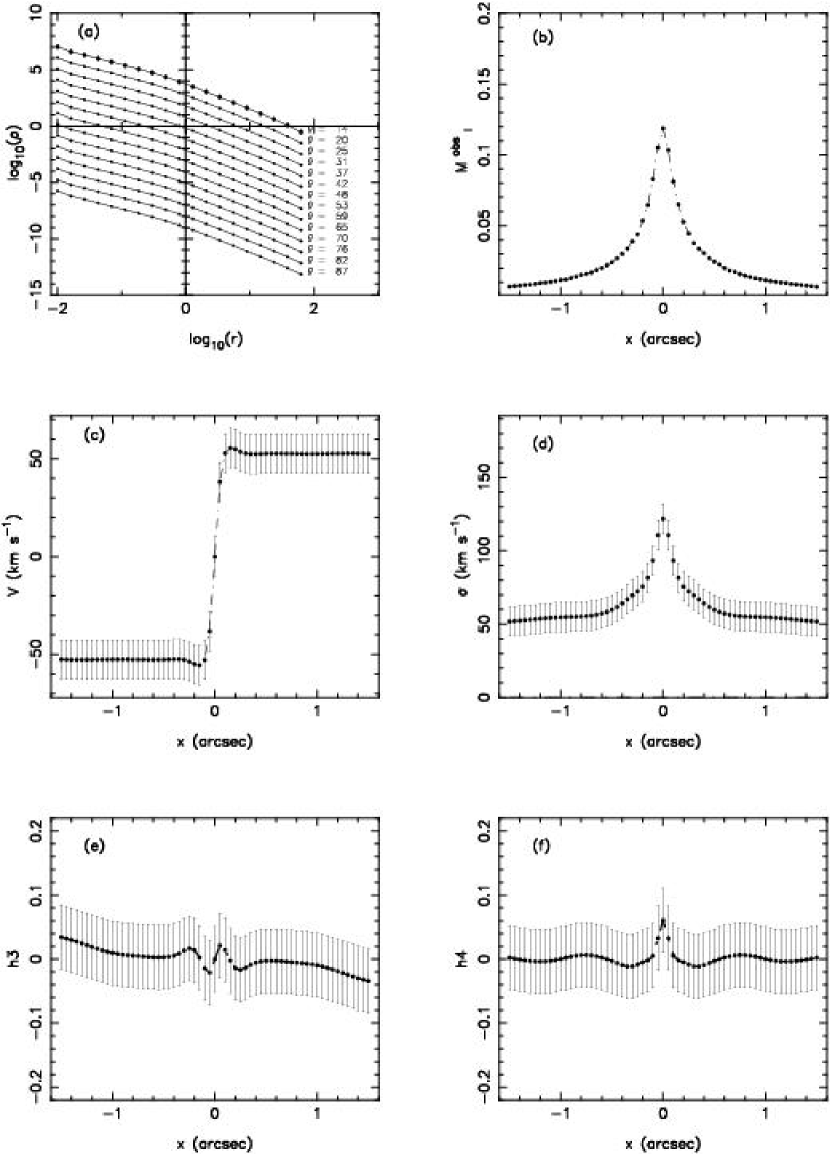
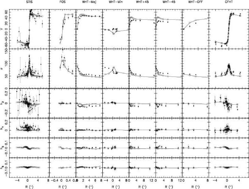
We first apply our modeling algorithm to various subsets of data set A. Data set A consists of kinematics within 1.5″, “observed” in such a way as to mimic observations of galactic nuclei with HST/STIS. In addition we include mass constraints out to 100″. Figure 1 shows the entire data set; the total number of constraints is 571. No regularization (smoothing) constraints were imposed in any of the models in this section.

In order to test the dependence of the modeling results on the number and type of data points supplied to it, we defined restricted data sets as follows:

a) A total of 98 constraints, consisting of the masses in 56 cells (every third radial cell and every third polar angle), and $v_{l}$ and $\sigma_{l}$ as measured in every third aperture.

b) A total of 164 constraints, consisting of the masses in 102 cells (every other radial cell and every other polar angle), and $v_{l}$ and $\sigma_{l}$ in 31 apertures.

c) A total of 226 constraints, consisting of the same mass constraints as in (b), as well as $v_{l}$, $\sigma_{l}$, and the GH moments $h_{3}-h_{4}$ measured at the same positions as in (b).

d) All 571 constraints, consisting of $19\times 14$ cell masses, and $v_{l}$, $\sigma_{l}$ and $h_{3}-h_{4}$ in all 61 apertures.

We did not explicitly include the aperture masses shown in Figure 1b ($M^{\rm obs}_{l}$) in the fits (although they are implicitly included as described in § 2.3.) However we verified that the aperture masses were always fitted to better than 0.1% for this data set.

Figure 2.— Contour plots of $\chi^{2}(M_{\bullet},\Upsilon)$ for models constructed to fit various subsets of data set A. The star indicates the true model parameters. Left column: The number of orbits used in the solutions was fixed at $N_{o}=1430$. (a) Fits to $v_{l}$ and $\sigma_{l}$ only, coarsely sampled; $N_{c}=98$. (b) $v_{l}$ and $\sigma_{l}$ only, finely sampled; $N_{c}=163$. (c) All four GH moments, finely sampled; $N_{c}=225$. (d) All four GH moments, very finely sampled; $N_{c}=571$. ($N_{c}$ includes mass constraints.) Right column: Fits were carried out using the same data as in the left column, but now the number of orbits has been varied in order to keep $N_{o}/N_{c}$ constant at 15.6. (e) $N_{o}=2451$ (f) $N_{o}=3412$ (g) $N_{o}=8928$. When the ratio of orbits to constraints is kept constant, increasing the number of data points has little effect on the tightness of the $\chi^{2}$ contours.

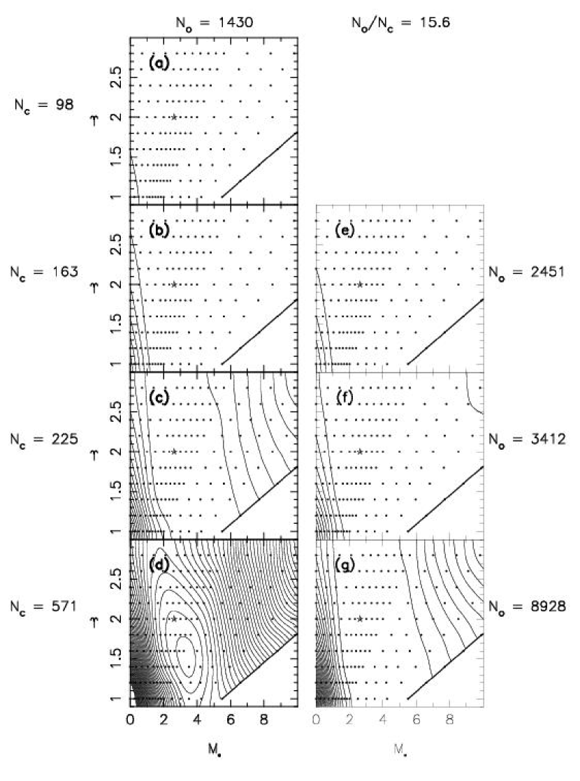
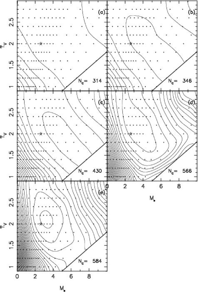
The left column of Figure 2 shows how the $\chi^{2}$ contours change as the number of constraints is increased, given a fixed number of orbits, $N_{o}=1430$. It is clear that the lowest velocity moments $v_{l}$ and $\sigma_{l}$ contain almost no information about $M_{\bullet}$ or $\Upsilon_{V}$: only when the higher GH moments are added do the $\chi^{2}$ contours begin to exhibit a definite minimum. However the best-fit parameters in Figure 2d are substantially displaced from their true values and plots of the predicted kinematics confirm that the fit to the data is poor.

Figure 3.— Contour plots for a fixed set of observational constraints (same as in Figure 2d, $N_{c}=571$) but different numbers of orbits, as indicated. The conclusions drawn from this data set about the best-fit model parameters $M_{\bullet}$ and $\Upsilon_{V}$ and their uncertainties would depend very strongly on the number of orbits used in the modeling. The properties of the models labelled $A$- $D$ are illustrated in Figure 6.

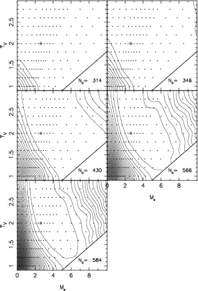
A possible explanation for the offset and for the poor fit when the number of data constraints is large, is the small ratio of orbits to constraints in Figure 2d, $N_{o}/N_{c}=2.5$. This modest ratio – while typical of the published modeling studies (e.g. vdM98) – suggests that our algorithm did not have much freedom to explore different orbital solutions. To test this idea, we repeated the experiments but this time increased the number of orbits in step with the number of constraints so as to keep the ratio $N_{o}/N_{c}$ fixed. The results are shown in the right panel of Figure 2. The differences are striking: we now see that the topology of the first set of contours was an artifact of the small number of orbits used. When the number of orbits is increased from 1430 to 8928 – i.e. when the ratio of orbits to constraints is increased from 2.5 to  15 – the minimum in $\chi^{2}$ disappears, leaving only a broad $\chi^{2}$ plateau. The true set of model parameters lies within this plateau although there is no sense in which this model can be said to be “preferred.” Evidently, even the full set of GH moments can only weakly constrain the potential when the modeling algorithm has the freedom to construct a wide variety of orbital populations. It must be emphasized that in the absence of smoothing constraints the actual number of orbits actually used by the optimization routine is roughly equal to the total number of constraints, irrespective of the size of the orbit library. Increasing the size of the orbit library basically increases the availability of orbits with the right kind of properties in the right part of phase space.

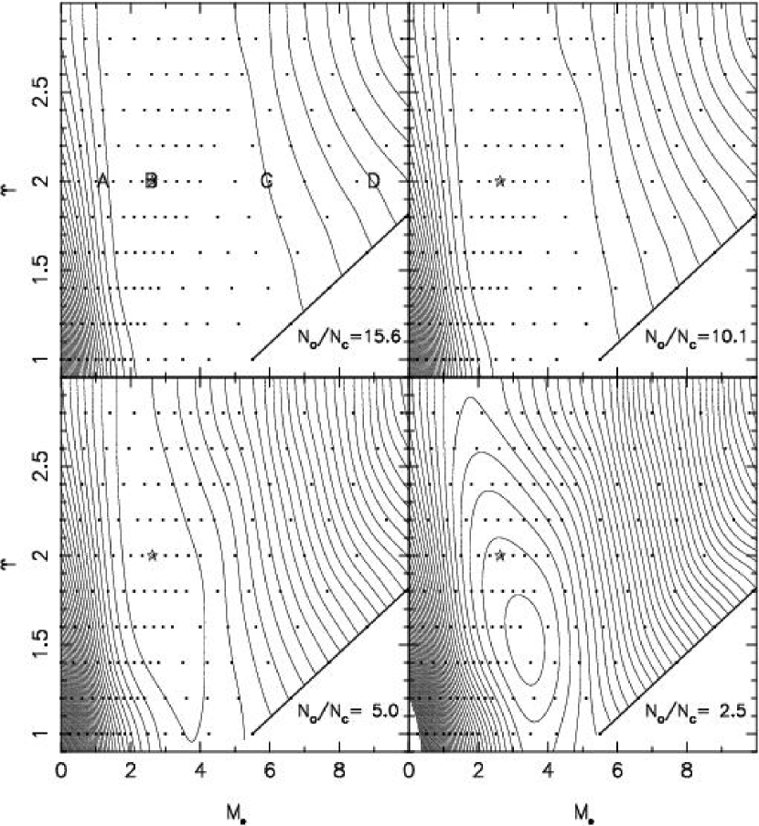
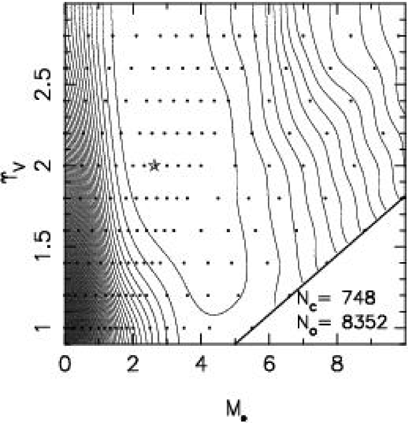
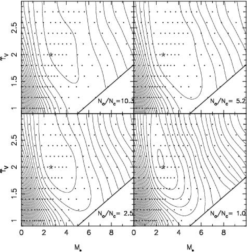
In these experiments, the number of observational constraints was varied. More typically one is faced with a fixed number of measurements. Figure 3 shows what happens when $N_{c}$ is fixed – we used the full data set A, with $N_{c}=571$ – but the number of orbits is varied. Again we see that the topology of the $\chi^{2}$ plot depends strongly on the ratio of orbits to constraints. As $N_{o}/N_{c}$ increases from 2.5 to 5.0, the $\chi^{2}$ contours shift so that their apparent center is close to the true model parameters, but as $N_{o}/N_{c}$ is increased still more, all semblance of a unique $\chi^{2}$ minimum vanishes and the potential parameters become essentially unconstrained. Indeed it is not clear from these plots whether we have reached a limit; the $\chi^{2}$ valley may become even broader as $N_{o}/N_{c}$ is increased above 15.6. In the plots with the two largest values of $N_{o}/N_{c}$, models lying within the $\chi^{2}$ plateau provide essentially perfect fits to the kinematical data and each of the mass constraints is fit to better than one part in $10^{6}$. Figure 4 shows the quality of the fit to the data in the cases $N_{o}/N_{c}=5.0$ and $2.5$; the most significant deviations are in $h_{4}$.

Figure 4.— Fits to the kinematical data (Fig. 1) for two orbital solutions that lie within the $\chi^{2}$ valleys of Fig. 3, close to the true model ($\star$). Solid line: $N_{o}/N_{c}=5$; dashed line: $N_{o}/N_{c}=2.5$. Models constructed using the two larger values of $N_{o}/N_{c}$ shown in Fig. 3 provide almost perfect fits to these data; those fits are not shown here.

Figure 5.— 1-D cuts through the $\chi^{2}$ plots of Fig. 3, all taken at $\Upsilon_{V}=2.$ The vertical arrow indicates the location of the true model parameter, $M_{\bullet}=2.625\times 10^{6}{{\cal M}_{\odot}}$. When the number of orbits used is small, there is a definite, but spurious, $\chi^{2}$ minimum. As $N_{o}$ is increased, this minimum broadens into the perfectly flat plateau characteristic of under-determined problems. The true model parameters lie on that plateau but can not be unambiguously recovered.

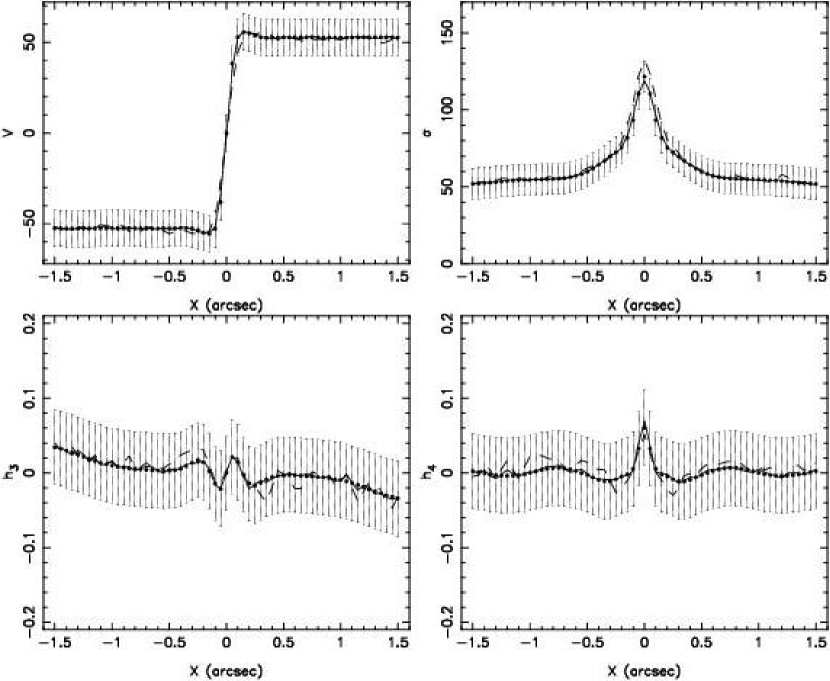
Figure 5 shows 1D cuts through the $\chi^{2}$ plots of Figure 3, all taken at $\Upsilon_{V}=2.$ As the ratio $N_{o}/N_{c}$ increases, two things happen: the absolute value of $\chi^{2}$ drops, reflecting the better quality of the fit as the number of orbits is increased; and the $\chi^{2}$-valley becomes broader. The plateau of precisely-constant $\chi^{2}$ predicted in §3 is very clear for $N_{o}/N_{c}\gtrsim 5$. The true value of $M_{\bullet}$ lies within this plateau but there is no sense in which it is preferred. This behavior of the $\chi^{2}$ plots as $N_{o}$ is varied was first predicted by Merritt & Ferrarese (2001) (their Fig. 7).

Figure 6.— The intrinsic velocity dispersions $\sigma_{r},\sigma_{\phi},\sigma_{\theta}$ as functions of radius for models A-D in Fig. 3. All models have comparable $\chi^{2}$ values and $\Upsilon_{V}=2$. Black hole masses are: A, $1\times 10^{6}{{\cal M}_{\odot}}$; B, $2.66\times 10^{6}{{\cal M}_{\odot}}$; C, $6.\times 10^{6}{{\cal M}_{\odot}}$; D, $8.5\times 10^{6}{{\cal M}_{\odot}}$. The values of $\Upsilon$ and $M_{\bullet}$ used in constructing Model B are closest to the true values. This model is approximately isotropic ($\sigma_{r}\approx\sigma_{\theta}$), as was the 2I model from which the data were generated.

The internal velocity dispersions in four models (labeled A-D in Figure 3a) are shown in Figure 6. The models all have $\chi^{2}$ values comparable to the model with the true potential parameters. Close to the center, the model with lowest $M_{\bullet}$ (A) has a significantly larger number of stars on radial orbits than the models with large $M_{\bullet}$ (C-D); the increase in $\sigma_{r}$ is needed to keep the central velocities high in spite of a too-small black hole. Nevertheless, so great is the freedom to choose different orbital populations that even knowledge of the projected GH moments can not rule out these extreme models.

Figure 7.— $\chi^{2}$ contours for fits to the data from data set A, to which has been added the simulated data from the “WHT” ground-based apertures.

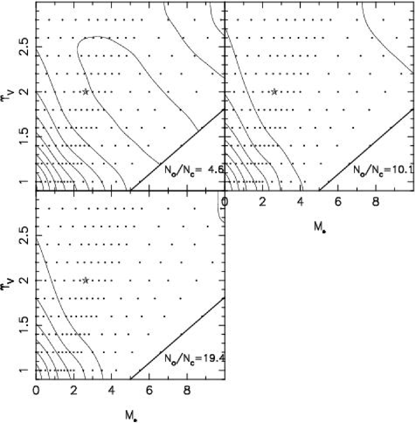
It is essential to point out that part of the indeterminacy illustrated in Figure 3 might be due to the fact that the data of data set A are restricted to the region near the black hole; hence the model kinematics are not at all constrained at large radii. This means that the modeling algorithm has unlimited freedom to vary the properties of the model at large radii while fitting the small radius data. In order to test if this is the sole cause of the indeterminacy we show in Figure 7 how the $\chi^{2}$ contours are modified if, in addition to data set A (kinematical data extending to 1.5″), the modeling algorithm is given the additional $44$ data points (including the first 4 moments of the LOSVD at each point) from data set B that correspond to the ground-based WHT observations along all position angles (kinematical data extending out to 8″). We see once again that when the full orbit library of $\sim 9000$ orbits is used a long flat $\chi^{2}$ valley which is somewhat more restricted in $M_{\bullet}$ results.

As an alternative to fitting GH moments, one can fit directly to the LOSVDs from which the GH moments were derived (e.g. Merritt (1997)). This procedure is expected to be inefficient if the LOSVDs are nearly Gaussian since measurements at many distinct velocities are required to reproduce accurate estimates of just the lowest-order GH moments. But direct use of the LOSVDs may be advisable near the centers of galaxies where observations can reveal extended wings due to high-velocity motion around the black hole (e.g. Joseph et al. (2001)), wings that are poorly represented by the lowest terms in a GH expansion.

Figure 8.— $\chi^{2}$ contours for fits to the full LOSVDs in all 61 apertures of data set A; $N_{c}=1198$. $N_{o}=8928,5775,2863,1430$ in a-d respectively.

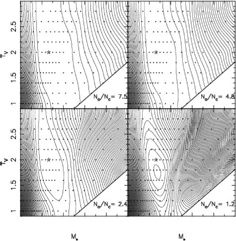
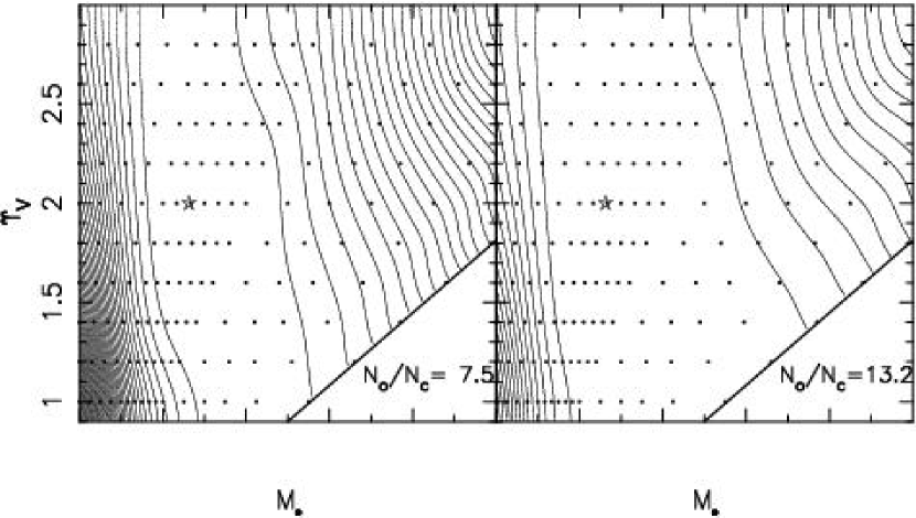
Figure 8 shows $\chi^{2}$ contours for fits to the full LOSVDs, sampled at $\Delta v\sim 40$km s^-1 . This velocity sampling is approximately equal to the velocity resolution of the STIS spectrograph at 8500Å. (The velocity scale of the the STIS spectrograph at $\sim 8500$Å  is $\sim 19$km s^-1 per pixel. Thus two pixels in the spectral direction (Nyquist sampling) imply a velocity resolution of $\sim 38$km s^-1  ). A more pragmatic justification is that sampling at $\Delta v\sim 40$km s^-1  already implies 1198 constraints and halving the velocity spacing would increase the number of constraints to over 1800, requiring a prohibitively large number of orbits for the modeling. We carried out optimizations for the same four sets of orbits ($N_{o}=8928,5775,2863,1430$) used to fit the GH moments in Figure 3. The total number of data constraints was 1198: the same set of 266 mass constraints as in Figure 3, and the LOSVDs measured at all 61 apertures along the major axis. The ratio $N_{o}/N_{c}$ is smaller than in the plots of Figure 3 because of the roughly three times larger number of constraints required to represent the LOSVDs.

Figure 9.— 1-D cuts through Figure 8 for $\Upsilon_{V}=2$. The unique minimum in $\chi^{2}$ that appears when the number of orbits is small, becomes a perfectly flat plateau when $N_{o}$ is large, indicating that the estimation of $M_{\bullet}$ from these data is under-determined.

In all four panels of Figure 8, the decrease in $N_{o}/N_{c}$ relative to Figure 3 results in a slightly smaller allowed range of models. But once again, for a large enough orbit library, there is an extended region within which $\chi^{2}$ is precisely constant. For the smallest orbit library ($N_{c}=1430$) the true solution lies outside the minimum contour and the “best fit” solution is obtained for a larger $M_{\bullet}$ and smaller $\Upsilon$ than those corresponding to the true solution. Figure 9 shows 1D cuts through Figure 8 for $\Upsilon_{V}=2$. The constant-$\chi^{2}$ plateau appears for $N_{o}/N_{c}\gtrsim 5$.

In order to make a more reasonable comparison between the quality of the fits to the LOSVDs and to the GH moments, we defined a new statistic $\chi^{2}_{\rm kin}$, which measures only the goodness of fit to the kinematical data in each aperture i.e. $V$, $\sigma$, $h_{3}$ and $h_{4}$, rather than the value of the objective function (which in this case includes the LOSVDs). (The $\chi^{2}$ of the fit to the mass constraints is also excluded from $\chi^{2}_{\rm kin}$ but is $<10^{-3}$ everywhere). When 8928 orbits were used, fitting to the LOSVDs gave a minimum $\chi^{2}_{\rm kin}=0.416$, while fitting to the GH moments gave $\chi^{2}_{\rm kin}=0.0442$. (Although there is nearly an order of magnitude difference in the two numbers, the two fits are indistinguishable to the eye and both are virtually perfect.) Thus we conclude that fitting to the GH moments may be adequate even when the LOSVDs have large wings, as in the case of our central aperture.

Prior to the installation of STIS aboard HST, the faint object spectrograph (FOS) was used to observe the nuclei of galaxies with high spatial resolution, although its velocity resolution was only $\sim 100$km s^-1 . Due to the difficulties associated with reducing the FOS data, only a few of the galaxies observed with the FOS have been modeled. These include M32 (vdM98) and NGC 3379 Gebhardt et al. 2000a . vdM98 used $V_{l}$ and $\sigma_{l}$ as derived from the FOS observations in their modeling of M32, while Gebhardt et al. (2000a) attempted to extract the central few LOSVDs in NGC 3379, sampled at 100 km s^-1  spacing. In their most recent paper Gebhardt et al. (2003) modeled the kinematics of 12 galaxies with nuclear data from STIS. In all cases they sample the LOSVDS with only 13 points with typical velocity spacing of $\sim 100$km s^-1 . In Figure 10 we compare the fits to LOSVDs sampled at 40 km s^-1  and 100 km s^-1  at all 61 apertures using the full orbit library of 8928 orbits. This plot shows that when LOSVDs are coarsely sampled with $\Delta v=100$km s^-1 , a much larger region of parameter space can fit the data equally well and the model parameters are not well constrained. Figure 11 shows 1D cuts through Figure 10 at $\Upsilon_{V}=2$. For the model closest to the “true” model ($M_{\bullet}=2.66$, $\Upsilon_{V}=2$), $\chi^{2}=0.416$ and $\chi^{2}=0.084$ for $\Delta v=40$km s^-1  and $\Delta v=100$km s^-1  respectively.

Figure 10.— Fits to the LOSVDs sampled with $\Delta v=40$ km s^-1  (left panel) and $\Delta v=100$ km s^-1 (right panel) at all 61 apertures using the full library of 8928 orbits.

Figure 11.— 1-D cuts through Figure 10 at $\Upsilon_{V}=2$. The solid line is for $\Delta v=40$ km s^-1  and the dashed line is for $\Delta v=100$ km s^-1 . Arrow marks true value of $M_{\bullet}$.

From these $\chi^{2}$ values, one might conclude that all models close to the bottom of the $\chi^{2}$ valley would give equally good fits. However, it is once again essential to compare how the kinematics would be fitted if all the information in the best sampled LOSVDs were used. To do this we use the orbital weights provided by the fits to the LOSVDs sampled at 40 km s^-1  and 100 km s^-1  but co-add the appropriately weighted GH moments computed from the orbital LOSVDs sampled at 5 km s^-1 . Figure 12 shows the fits the GH moments for models lying on the plateau of the $\chi^{2}$ valley with each of the two velocity spacings. It is clear that fitting coarsely-sampled LOSVDs gives a much poorer fit to the kinematical data, especially for the higher-order GH moments, e.g. $h_{4}$. This is despite the fact that they are an almost perfect fit to the coarsely sampled LOSVDs! This quality of the fit worsens even more at points further away from the true model as shown by the steeply rising and highly variable $\chi^{2}_{\rm kin}$ values plotted in Figure 13. This is understandable since both $V$ and $\sigma$ at large radii are $\sim 50$km s^-1 roughly half the spacing between points in the LOSVD!

Figure 12.— Fits to the kinematical data ($V_{l},\sigma,h_{3},h_{4}$)) for models from Fig. 10 with $M_{\bullet}=2.66$, $\Upsilon_{V}=2$. The solid line is the fit obtained with $\Delta v=40$km s^-1 ($\chi^{2}_{\rm kin}=4.16\times 10^{-1}$) and the dashed line is the fit obtained with $\Delta v=100$km s^-1 ($\chi^{2}_{\rm kin}=32.5$).

Figure 13.— 1-D plot of $\chi^{2}_{\rm kin}$ for $\Upsilon_{V}=2$ for fits with the two different velocity spacings ($\Delta v=40$km s^-1 and $\Delta v=100$km s^-1 ).

The suitability of LOSVDs sampled at $\sim 100$km s^-1 is likely to be particularly bad in compact low luminosity ellipticals like M32 where the central velocity dispersion is $\leq 150$ km s^-1 but may be less problematic in large giant ellipticals where the central velocity dispersion is $\sim 250-300$ km s^-1 . It is clear however that using a fixed number of grid points per LOSVD for all galaxies could produce non-uniform results. This implies that it is essential to tailor the modeling parameters to each galaxy.

6. Fits to Data Set B – A 2I Model of M32

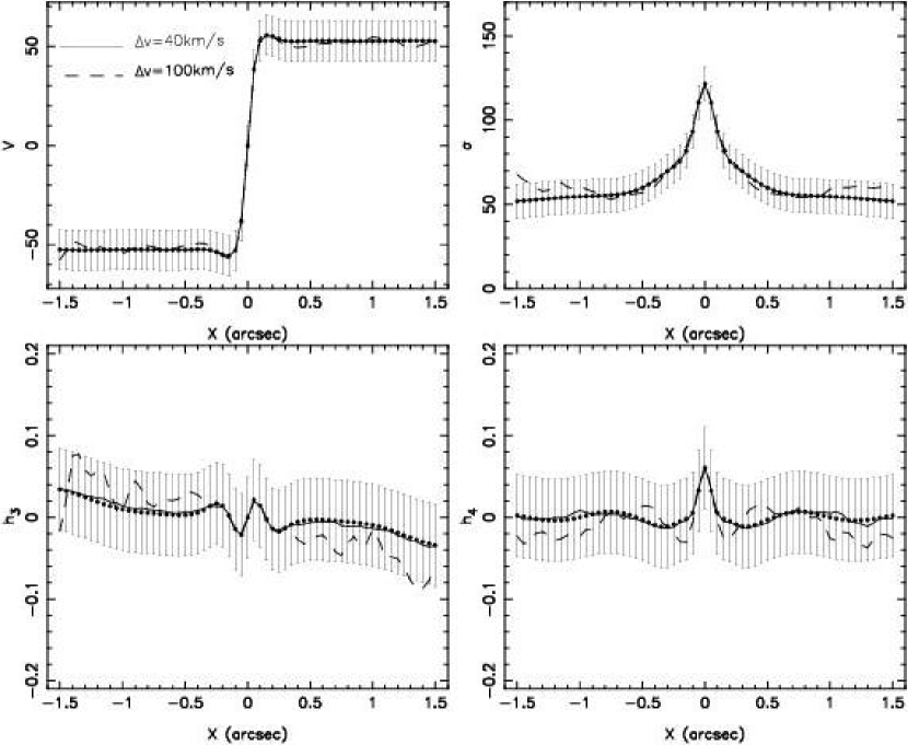
Data set B was obtained by “observing” the 2I model through exactly the same set of apertures, and with the same PSFs, as in the observations of M32 (van der Marel et al. 1994a; Bender et al. 1996; vdM98; Joseph et al. 2001) that were used to construct the 2I model described in section § 3. vdM98 used this same set of observations in building their 3I models of M32 and estimating the black hole mass. Figure 14 shows that data set B is not a perfect match to the actual M32 data although it reproduces the kinematics near the central black hole very well. Error bars on the pseudo dataset were defined as described in § 4.

Figure 14.— Data set B. Solid dots represent the real data to which the 2I model was fitted; solid lines represent the 2I fit; open squares represent the points on the fit which were selected as data set B.

In Figure 15, we repeat an experiment first carried out by vdM98 in their analysis of the actual M32 data (see their Appendix A). We fixed the number of orbits in our 3I modeling algorithm at $N_{o}=1982$ – similar to the number (1960) used by those authors – and explored how the $\chi^{2}$ contours change as we apply progressively larger numbers of observational constraints, as follows (all from data set B): (a) major axis $V$ and $\sigma$ in the WHT and CFHT apertures; (b) major axis $V$, $\sigma$, $h_{3}$, $h_{4}$ (WHT, CFHT); (c) major and minor axis $V$, $\sigma$, $h_{3}$, $h_{4}$ (WHT, CFHT); (d) $V$, $\sigma$, $h_{3}$ and $h_{4}$ along all position angles (WHT, CFHT); (e) all constraints in (d) plus $V$ and $\sigma$ from the HST/FOS apertures. Each of these fits included 266 meridional-plane mass constraints within 100″.

Figure 15.— Contour plots of the $\chi^{2}$ that measures the quality of the fit to various subsets of data set B (the simulated M32 data) using 1982 orbits. (a) Major axis $V$ and $\sigma$ (WHT, CFHT apertures); (b) major axis $V$, $\sigma$, $h_{3}$, $h_{4}$ (WHT, CFHT apertures); (c) major and minor axis $V$, $\sigma$, $h_{3}$, $h_{4}$ (WHT, CFHT apertures); (d) $V$, $\sigma$, $h_{3}$, $h_{4}$ along all PAs (WHT, CFHT apertures); (e) all of the constraints in (d) plus $V$ and $\sigma$ from the FOS apertures. The $\star$ labels the true model parameters. $N_{c}$ is the total number of constraints including mass constraints. This plot seems to suggest that the constraints on $M_{\bullet}$ and $\Upsilon$ become rapidly tighter as the number of data points increases.

As in the previous section none of the models discussed in this section were constructed with regularization constraints imposed.

Figures 15 and 16 show how the constraints on $M_{\bullet}$ and $\Upsilon$ appear to tighten as the number of data points provided to the modeling algorithm are increased. When only the major-axis “WHT” measurements of $V$ and $\sigma$ are used, the potential parameters are almost unconstrained, but when the entire data set is given to the modeling algorithm, a well-defined minimum appears in $\chi^{2}(M_{\bullet},\Upsilon)$ that is reasonably close to the true model parameters. vdM98 found a similar dependence of the $\chi^{2}$ contours on number of data points when modeling the true M32 data.

Figure 16.— 1-D cuts through Figure 15 at $\Upsilon_{V}=2$. Arrow indicates true value of $M_{\bullet}$.

But Figures 17 and 18 tell a very different story. Now the fits have been carried out using a fixed ratio of orbits to data constraints, $N_{o}/N_{c}\approx 10$. The rapid shrinking of the $\chi^{2}$ contours with increasing $N_{c}$ in Figure 15 and 16 is now gone: even using the full set of data gives a $\chi^{2}(M_{\bullet})$ plot with an extended flat plateau, stretching from $M_{\bullet}\approx 2\times 10^{6}{{\cal M}_{\odot}}$ to $M_{\bullet}\approx 6\times 10^{6}{{\cal M}_{\odot}}$. The true value, $M_{\bullet}=2.625\times 10^{6}{{\cal M}_{\odot}}$, lies on the edge of this plateau suggesting that even the large number of orbits we used (5856) is barely sufficient to reproduce the true $\chi^{2}$ contours.

Figure 17.— Same as Figure 15, except that the size of the orbit library in each panel has been adjusted such that $N_{o}/N_{c}$ is constant at $\sim 10$. The $\chi^{2}$ contours now change much more slowly as the number of data points is increased, and even for the full data set, the constraints on $M_{\bullet}$ and $\Upsilon$ are weak.

Figure 18.— 1-D cuts through Figure 17 at $\Upsilon_{V}=2$. Even using the full data set ($N_{c}=584$), there is a plateau of constant $\chi^{2}$ indicating that these simulated data do not uniquely constrain $M_{\bullet}$.

The most important conclusion we draw from a comparison of Figures 15 and 17 is that the appearance of the $\chi^{2}$ contours depends strongly on the flexibility of the modeling algorithm. The quality of the fit to the data depends at least as strongly on the size of the orbit library as on the size of the data set. Comparisons between fits made with different sets of data are problematic unless care is taken to demonstrate that the ratio $N_{o}/N_{c}$ is sufficiently large for each fit. And for a given data set, statements about the best-fit model parameters and their confidence intervals can be very strongly influenced by the number of orbits used.

We note that including the “HST/FOS” measurements from data set B has almost no influence on the range of indeterminacy in $M_{\bullet}$; the width of the constant-$\chi^{2}$ plateau is virtually unchanged (Figure 18). This suggests that the FOS data for M32 did not significantly tighten the constraints on the mass of the black hole in this galaxy compared with the constraints set by the ground-based data. vdM98 reached a different conclusion; comparison of Figures 15 and 17 suggests that they may have been misled by the relatively small number of orbits in their modeling algorithm.

Figure 19.— Fits to the subset of data set B corresponding to the ground-based, WHT apertures only, for various numbers of orbits; $N_{c}=430$.

Figure 20.— 1-D cuts through Figure 19 at $\Upsilon_{V}=2$. These data, which are superior in quality to most STIS/HST nuclear data, place only very weak constraints on $M_{\bullet}$.

It is interesting to compare these results with those obtained using only the subset of data set B corresponding to the ground-based, WHT data; these (simulated) data have an effective resolution ${\rm FWHM}/2r_{h}\approx 0.5$, better than that of most galaxies observed with HST/STIS (Merritt & Ferrarese 2001b ; Gebhardt et al. (2003)) and their spatial coverage and S/N are much greater than those of most STIS nucleus data. Thus we extracted from data set B measurements at all the WHT apertures of $V$, $\sigma$, $h_{3}$ and $h_{4}$, including all position angles (430 constraints). Figures 19 and 20 show the results, for three different numbers of orbits, $N_{o}=(1982,5674,8352)$. When the ratio of orbits to constraints is largest ($N_{o}/N_{c}=19.4$ for $N_{o}=8352$), excellent fits are obtained for any black hole mass in the range $1\times 10^{6}{{\cal M}_{\odot}}\lesssim M_{\bullet}\lesssim 10\times 10^{6}{{\cal M}_{\odot}}$! While there is a hint of a minimum at $M_{\bullet}\approx 4.5\times 10^{6}{{\cal M}_{\odot}}$, it is well removed from the true value of $M_{\bullet}$ and furthermore its location is very sensitive to $N_{o}$. We conclude that these data are almost useless for constraining the black hole mass. We would expect a similar or greater degree of indeterminacy in values of $M_{\bullet}$ derived from many of the galactic nuclei observed with HST/STIS. We return to this point in § 8.

Figure 21.— Contour plots of $\chi^{2}$ for models constructed to fit data set B including HST/STIS apertures as well. The same number of constraints (810) are fitted in each panel but the number of orbits in the library is varied as indicated on the plots.

Finally we ask if the constraints on $M_{\bullet}$ using this data set can be narrowed by adding the simulated HST/STIS data. Figure 21 shows $\chi^{2}$ contours for 3I model fits to data set B including all the STIS apertures as well as the ground based and FOS apertures. The data were fitted at 140 apertures in total (the four outermost STIS data points on one side of the galaxy were the only apertures in the Joseph et al. (2001) data set that were not fitted). Figure 22 shows 1-D cuts through the $\chi^{2}$-contour plot at $\Upsilon=2$. This figure suggests that the addition of the STIS data to the existing data for M32 may yield a tight constraint on $M_{\bullet}$: even for the largest orbit library, the allowed range of solutions is quite small. We note also that the true solution lies close to the center of the minimum in the $\chi^{2}$ valley.

Figure 22.— 1-D cuts through Fig. 21. This figure shows that for the largest orbit library, the minimum in the $\chi^{2}$ valley is still reasonably narrow, suggesting that the HST/STIS data for M32 may yield tight constraints on $M_{\bullet}$ in this galaxy.

Figure 21(a) should be considered provisional since the ratio of orbits to constraints is $\sim 10$ and likely to be marginally adequate. We will return to this point in a later paper when we analyze the observed STIS data for M32.

7. Data Set C: M32 Re-Examined

In § 5 and 6 we presented $\chi^{2}$-plots of fits to two simulated data sets derived from a model that was based on data from M32. Here we show the results of fits to the actual data used in the construction of that model, our data set C. These are the same data used by vdM98 in their 3I study of M32. The constraints in our data set C include meridional plane masses in 266 cells. In the modeling results presented below, mass constraints were fit to an accuracy of better than 3% everywhere and to better than 0.1% at all points within the minimum $\chi^{2}$-valley.

The models discussed in this section were constructed without regularization constraints. The same is true of the vdM98 modeling of M32 with which we make comparisons. Our conclusions about the robustness of those authors’ results with regard to size of orbit library are therefore unaffected by questions of regularization.

Figure 23.— Contour plots of the $\chi^{2}$ that measures the quality of the fit to the combined FOS, CFHT and WHT data sets for M32. These are the same data fitted by van der Marel (1998) in their 3I modeling study. M32 is assumed to be edge-on. The four panels show the results using four different sizes of orbit library. Model parameters are the black hole mass $M_{\bullet}$ in $10^{6}{{\cal M}_{\odot}}$ and the $V$-band mass-to-light ratio $\Upsilon$ in solar units. Dots indicate models that were calculated. Labelled positions are models whose fit to the data is illustrated in detail in Figure 25. The upper right panel is based on the same number of orbits as in van der Marel et al. (1998) and shows two distinct $\chi^{2}$ minima, as in their paper. As the number of orbits is increased, these two minima merge and broaden into a plateau of constant $\chi^{2}$.

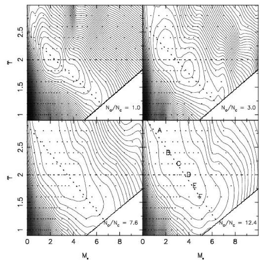
Figure 23 shows the results of fitting the full data set using four different orbit numbers, $N_{o}=(665,1999,5127,8352)$, or $N_{o}/N_{c}=(1.0,3.0,7.6,12.4)$. The top-right-hand panel of Figure 23 was made using almost exactly the same number of orbits as in vdM98. This plot exhibits two minima in $\chi^{2}(\Upsilon,M_{\bullet})$; the corresponding plot in vdM98 (their Fig. 6) also shows two minima, although displaced slightly from the two in our Figure 23b. However as $N_{o}$ is increased, we find that the two minima merge into a single, broad plateau.

In their edge-on modeling of M32 from these data, vdM98 selected a model with $M_{\bullet}=3.4\times 10^{6}{{\cal M}_{\odot}}$ and $\Upsilon\approx 2$ as their best fit. That model lies between the two minima seen in the upper-right panel of Figure 23 and somewhere near the center of the constant-$\chi^{2}$ plateau in the lower panels. It is important to note that the approximate agreement with the results of vdM98 is a valuable test of our code. The fact that the contours of vdM98 are not reproduced exactly are a result of discretization and differences in the details of the modeling which tend to be more obvious since the solutions depend on the small numbers of orbits used ($\sim 2000$).

Figure 24.— 1-D $\chi^{2}$ plots along the dotted lines in Figure 23. (a) Horizontal cut; (b) slanted cut. The four lines in each plot correspond to the four different numbers of orbits used in the modeling, increasing downward (cf. Figure 23). These plots show that the local minima appearing for small $N_{o}$ disappear as $N_{o}$ is increased, yielding a region of nearly constant $\chi^{2}$ stretching at least from $\sim 1\times 10^{6}{{\cal M}_{\odot}}$ to $\sim 6\times 10^{6}{{\cal M}_{\odot}}$.

In Figure 24 we present cuts along two axes in the $\chi^{2}(\Upsilon,M_{\bullet})$ plots (indicated by the dotted lines in Figure 23). One cut is at $\Upsilon=2$ and the other cut lies roughly along the minimum of the $\chi^{2}$-valley. These figures demonstrate that for the largest values of $N_{o}/N_{c}$ no preferred value for $M_{\bullet}$ in M32 can be found over a range in values that extends at least from $\sim 1.5\times 10^{6}{{\cal M}_{\odot}}$ to $\sim 5\times 10^{6}{{\cal M}_{\odot}}$.

Figure 25.— Predictions of selected models from Figure 23 compared with a subset of the M32 data. Models A-F have black hole masses ranging from $1.4\times 10^{6}{{\cal M}_{\odot}}$ (Model A) to $4.8\times 10^{6}{{\cal M}_{\odot}}$ (Model F). All plots show fits to major-axis data; however note that data along other position angles were also used in constructing the models and the $\chi^{2}$ values plotted in Figure 23 include the full data. There is very little difference in the quality of fit of these models to the CFHT and WHT data. The only visual difference is between the fits to the FOS data. The wildly varying velocity dispersions for the FOS data make this harder to fit. These plots along with Table 1, show that black holes with masses in the range $1.4\times 10^{6}{{\cal M}_{\odot}}<M_{\bullet}<4.8\times 10^{6}{{\cal M}_{\odot}}$ are equally consistent with the data.

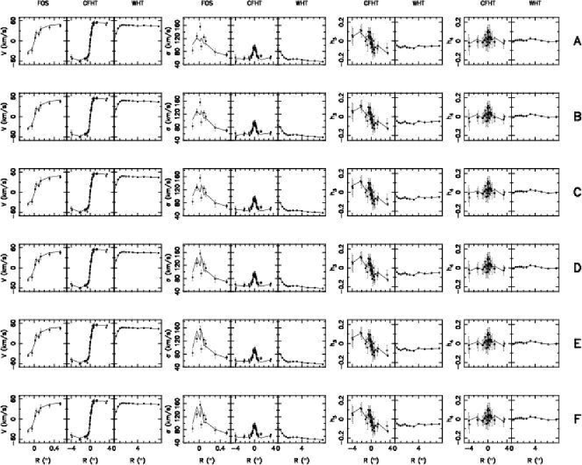
We demonstrate the indeterminacy even more clearly in Figure 25, which shows detailed fits to the kinematics for a set of models lying along the $\chi^{2}$ plateau in Figure 23. The differences between the various models – which span a range of almost a factor of four in $M_{\bullet}$ – are almost invisible, with the exception of the predicted values of $\sigma$ in the FOS apertures. This could be interpreted to mean that the FOS data contain useful information about $M_{\bullet}$, but we consider this unlikely, since none of the models fits the FOS data well, due to the large point-to-point fluctuations in the FOS velocity dispersions. It is entirely possible that smoother data, with the same spatial resolution as the FOS data, could have been fit well by all the models in this set.

Table 1$\chi^{2}$ of fit to individual datasets.

Model	$M_{\bullet}$	$\Upsilon_{V}$	$\chi^{2}_{\rm FOS}$	$\chi^{2}_{\rm CFHT}$	$\chi^{2}_{\rm WHT}$	$\chi^{2}$
A	1.4	2.8	22.45	49.24	39.55	111.19
B	2.4	2.4	22.88	49.32	28.36	100.56
C	3.3	2.2	25.17	51.33	26.51	103.01
D	4.0	2.0	30.96	46.97	28.11	106.04
E	4.5	1.8	32.88	49.38	27.30	109.56
F	4.8	1.6	33.90	50.20	25.88	109.98

In order to make the case for indeterminacy in $M_{\bullet}$ even more airtight, we present in Table 1 the contribution to $\chi^{2}$ from each of the three partial datasets (FOS, CFHT, WHT) that make up our data set C. The values of $\chi^{2}_{\rm CFHT}$ appear to fluctuate randomly from model A through F with no systematic behavior. By contrast, $\chi^{2}_{\rm FOS}$ is smallest for Models B and A and increases steadily toward larger $M_{\bullet}$. The opposite trend is observed for the fit to the WHT data; as a result, the total $\chi^{2}$ remains almost precisely constant. (Mass constraints contribute almost nothing to the total $\chi^{2}$ since they are fitted to better than 0.1% accuracy at all points within the minimum $\chi^{2}$-valley.) Although the lower values of $M_{\bullet}$ provide the lowest $\chi^{2}_{\rm FOS}$ they require too large a value of $\Upsilon$ to fit the large radius data. However the relative difference between models A and B or F and B is statistically insignificant.

Figure 26.— Intrinsic 3-D kinematics along the major axis for each of the models A-F. Black hole masses ranging from $1.4\times 10^{6}{{\cal M}_{\odot}}$ (Model A) to $4.8\times 10^{6}{{\cal M}_{\odot}}$ (Model F).

The internal kinematics of our models must vary with $M_{\bullet}$ and $\Upsilon$ in order to maintain fixed observables. Figure 26 shows plots of the major axis, internal velocity dispersion components for models A through F. The behavior is precisely as expected: near the center, models with lower $M_{\bullet}$ maintain a high central velocity dispersion by putting the largest fraction of stars on radial orbits; at high $M_{\bullet}$, the central line-of-sight dispersion is maintained by transferring more and more stars to nearly circular orbits around the black hole.

8. The Effect of Adding Regularization Constraints

In order to test the effect on the solutions of adding smoothness constraints, we ran a series of models to fit the full set of kinematical and mass constraints for pseudo data set B, with various values of the smoothing parameter $\lambda$ in equation (14). In this set of runs, the errors on the data were selected to be the same as those of the real data. Since regularization is computationally expensive, we ran this series of models with only 5000 orbits instead of the full orbit library.

Figure 27.— Plots of $\chi^{2}$ versus $M_{\bullet}$ and for $\Upsilon_{V}=2$ for a sequence of smoothing parameters ($\lambda$). The quantities $\Pi$ and $scale$ are defined in the text. In each plot the arrow marks the position of the “true value of $M_{\bullet}$”. At each data point the height of the bar is $\propto(\Pi-\Pi_{\rm min})/(\Pi_{\rm max}-\Pi_{\rm min})$ for the model.

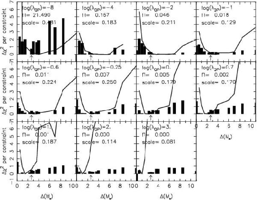
Each plot in Figure 27 shows $\chi^{2}$ per constraint versus $M_{\bullet}$ for $\Upsilon_{V}=2$. For each choice of ($M_{\bullet},\Upsilon_{V}=2$), the average level $\Pi$ of noise in the solution was computed via equation (2.4) in § 2.4 and the value of $\Pi$ is indicated by the height of the solid bar at each point. Since $\Pi$ varied by more than four orders of magnitude as $\lambda$ was varied, the height of the bar has been rescaled in each plot as $(\Pi_{i}-\Pi_{min})/\Pi_{min}$. In addition the plots give the quantities $scale=(\Pi_{max}-\Pi_{min})/\Pi_{min}$ and $\Pi$, the mean of all the noise values in a given plot. Arrows in each plot mark the position of the true value of $M_{\bullet}$.

The primary conclusion to be drawn from Figure 27 is that adding regularization constraints does not suddenly or dramatically reduce the degeneracy in $M_{\bullet}$. Although the mean level of noise ($\Pi$) drops by a factor of $\sim 500$ as $\lambda$ increases from $\lambda=10^{-8}-10^{-2}$, the flat $\chi^{2}$ plateau persists over this range with negligible decrease in the width of the plateau. There is no indication that the algorithm achieves good fits for incorrect values of $M_{\bullet}$ by selecting spuriously noisy solutions. Indeed, the noise level is roughly constant along the constant-$\chi^{2}$ plateaus, and rises sharply only outside; we provisionally interpret this to mean that all solutions along the plateau are “equally good” and that the algorithm does not need to construct highly artificial solutions in order to achieve its good fits. As $\lambda$ is increased beyond $\sim 1$, the extended plateau is replaced by a true minimum in $\chi^{2}$; this is a necessary consequence of the smoothness constraint, which begins to penalize solutions characterized by sharp phase-space gradients, even if they reproduce the data. However, the regularization does not seem to have any special ability to select out the correct $M_{\bullet}$: instead, as $\lambda$ is increased, the best-fit $M_{\bullet}$ systematically drops. This is also expected, since there is no reason for the true solution to also be the “most smooth” as defined by any particular choice of penalty function.

Figure 28.— Variation of the mid point of the $\chi^{2}$ valley as a function $\log(\lambda)$. Error bars indicate the range within which $\Delta\chi^{2}=0.5$. The broken line represents the “true” value of $M_{\bullet}$ for the pseudo data.

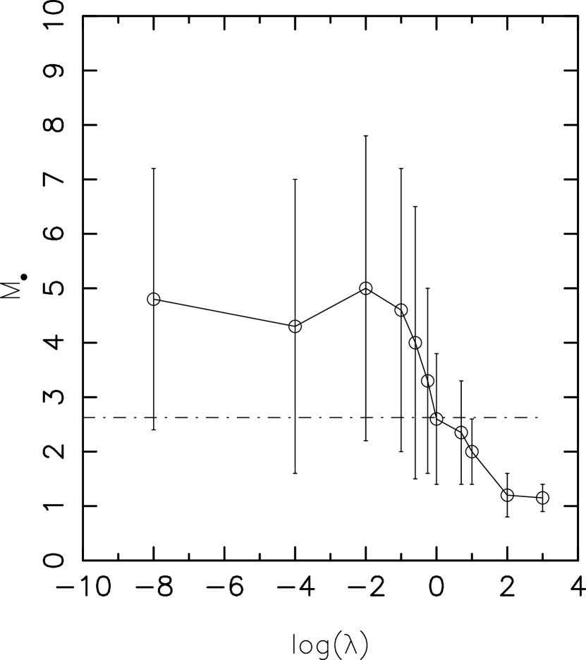
Figure 28 shows how the best-fit value of $M_{\bullet}$ and the range of acceptable $M_{\bullet}$ values varies with the level of imposed smoothing. We defined the range in $M_{\bullet}$ by $\Delta\chi^{2}=0.5$. For small values of $\lambda$, there is no well-defined minimum in $\chi^{2}$ and we defined the best-fit value as the value of $M_{\bullet}$ at the center of the $\Delta\chi^{2}=0.5$ region. While there does exist a particular value of $\lambda$ ($\lambda\approx 1$) for which the best-fit $M_{\bullet}$ is close to the input value, there would seem to be no way to guess this value based only on a plot like Figure 28. When $\log\lambda$ is increased just slightly above this value, the best-fit $M_{\bullet}$ drops below its true value as the smoothness constraint begins to bias the solution toward overly-smooth phase space distributions. In other words, the optimal value of $\lambda$ is only slightly smaller than the value at which the solutions begin to be seriously biased.

Several authors have based their choice of an optimal smoothing parameter on the ability of their algorithm to reproduce a specific 2I distribution function (e.g. Gerhardt et al. 1998, Cretton et al. 1999, Verolme & de Zeeuw 2002). There are two potential problems with this approach: first it has been shown that even for a known distribution function, the optimal value of $\lambda$ depends on the choice of data set (e.g. Cretton et al. 1999); second this choice of $\lambda$ is not guaranteed to give the underlying distribution function - but just one of the 3I distribution functions that is close to a 2I form. This is unlikely to be useful in the general case where the distribution function could deviate significantly from the 2I form. One might be particularly concerned about its applicability in modeling integral field data for galaxies with significant non-2I features: (counter rotating disks, cores etc). In such cases the use of a smoothing parameter optimized to recover a 2I distribution function could artificially restrict the models.

Figure 29.— 2-D $\chi^{2}$ contour plots for 3 different values of smoothing parameter $\log(\lambda)$ as indicated. The contours represent values of $\Delta\chi^{2}=\chi^{2}-\chi^{2}_{\rm min}$ with the minimum contour at $\Delta\chi^{2}=0.5$. Subsequent contours are at intervals of $\Delta\chi^{2}$ as indicated in the text. The grey scale represents the noise. In each plot white represents the least noisy model and black represents the most noisy model. As before the star indicates the position of the “true model”.

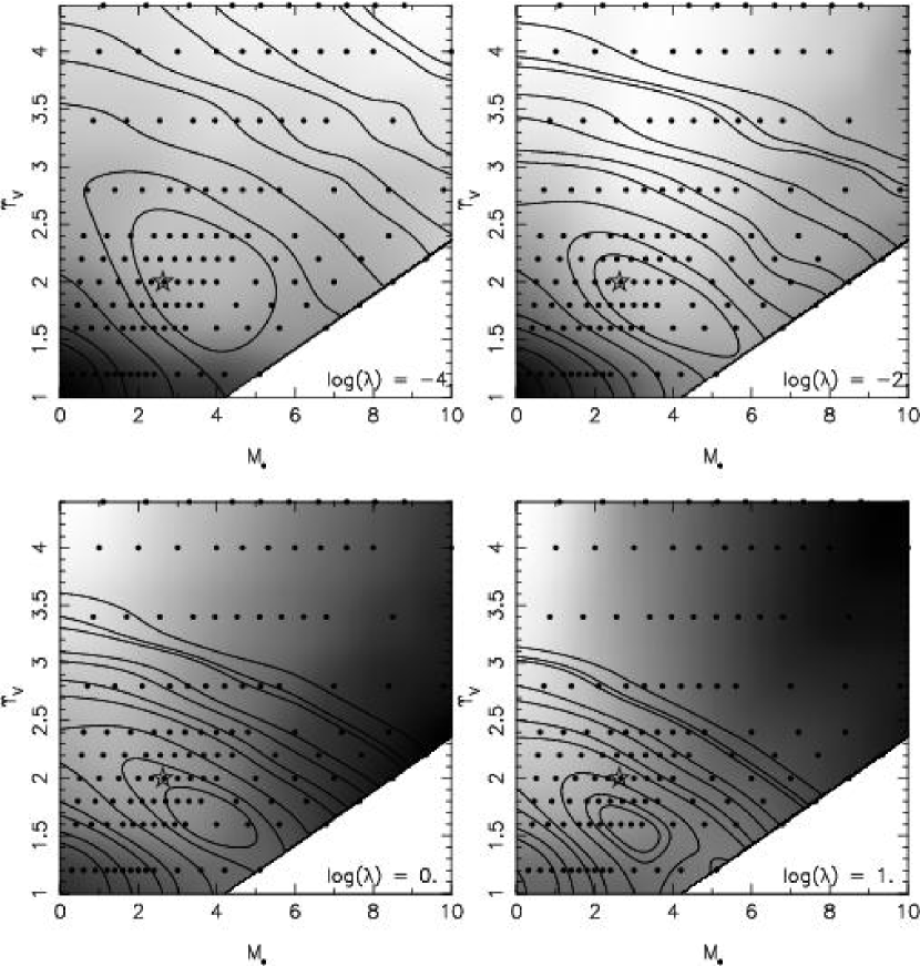
In Figure 29 we plot full $\chi^{2}$ plots for 4 values of $\log(\lambda)$. The contours trace the value of $\Delta\chi^{2}=(\chi^{2}-\chi^{2}_{\rm min})$. The first two contours are at $\Delta\chi^{2}=0.5,1.$ Subsequent contours are at spacings of $\Delta\chi^{2}=2.3,4.6,6.2,9.2,11.8,18.4$, which are the 68.3%, 90%, 95.4%, 99% 99.73% and 99.99% confidence regions on $M_{\bullet}$ and $\Upsilon_{V}$ jointly Press et al. (1992). The grey scale represents the noise. In each plot white represents the least noisy model and black represents the most noisy model. As in the case of the 1-D $\chi^{2}$ plots it is evident that an elongated $\chi^{2}$ minimum persists in both parameters even with moderate to high levels of smoothing. Once again, noise values do not appear to vary much within the minimum valley and are comparably low through the entire $\Delta\chi^{2}=0.5$ contour. There is also no indication that the models at the extremes of the contours are significantly more noisy than the models at the center. The regions with the largest amount of noise are also the regions where the $\chi^{2}$ values are very large. Interestingly for models at the top right of the plot, the $\chi^{2}$ values are large but the models have little noise. There appears to be little if any correlation between the noise levels and the distance from the $\chi^{2}$ valley.

These experiments are consistent with the view that the potential estimation problem is inherently ill-conditioned, and that regularization while it can artificially reduce the solution space can not overcome the degeneracy. We note a subtle but important distinction here between the role of smoothing in 2I and 3I modeling. In the 2I case, there does exist a unique (smooth) $f$ corresponding to any assumed potential, and the imposition of smoothing constraints might be expected to assist in the recovery of that unique $f$ (Merritt & Fridman (1996); Jalali & de Zeeuw (2002);Verolme & de Zeeuw (2002);
Cretton & Emsellem (2003)). Something similar must happen in the 3I case, but as our experiments show, the additional freedom associated with a 3I $f$ allows many potentials to be fit with orbital-space populations that are comparably smooth. This is just what one expects when solving an under-determined problem: smoothing alone can not overcome the degeneracy. Furthermore, as Figure 28 shows, there is a real danger associated with regularization: if the smoothing parameter is too large, the best-fit $M_{\bullet}$ is biased. Indeed this figure suggests that any $\lambda$ large enough to give a “best-fit” $M_{\bullet}$ – i.e. a unique minimum in $\chi^{2}$ – is also large enough to bias the location of that minimum. Hence the conservative approach to modeling would be to use little or no regularization, even if doing so means that no “best-fit” potential parameters will be found.

Finally, we note here a formal similarity between the various sorts of “constraint” that can be imposed on $f$. Forcing $f$ to depend only on $E$ and $L_{z}$; restricting the number of orbits from which a 3I $f$ is constructed; or forcing $f$ to be smooth, via some regularization scheme, all have the effect of artificially removing the degeneracy in the potential estimation problem, and converting flat $\chi^{2}$ contours into contours with a unique minimum. We consider each of these approaches to be dangerous. While any combination of $\Phi$ and $f$ that fits the data is acceptable, statements about the range of acceptable potentials depend critically on how flexible the modeling algorithm is at representing different forms of $f$. This consideration is particularly important when attempting to estimate the value of $M_{\bullet}$ in galactic nuclei, since artificially restricting $f$ may give the mistaken impression that a particular value of $M_{\bullet}$ is preferred, when in a fact a model with $M_{\bullet}=0$ can fit the data equally well.

9. Discussion

We have shown that the results obtained from stellar dynamical modeling of galaxy centers can depend as strongly on the flexibility of the modeling algorithm as on the number and nature of the observational constraints. Estimation of the parameters $M_{\bullet}$ (black hole mass) and $\Upsilon$ (stellar mass to light ratio) that define the gravitational potential is typically an under-determined (degenerate) problem, and 3I (three-integral) modeling can (and, we believe, often does) generate spurious, “best-fit” model parameters that bear no special relation to the true parameters. We demonstrated this in the case of previously-modeled data for M32: increasing the number of orbits by a factor of $\sim 4$ above what was used in the earlier studies led us to substantially different conclusions about the most likely value of the black hole mass and its uncertainty in this galaxy. Indeed, we found that no single value of $M_{\bullet}$ was preferred and that values for $M_{\bullet}$ in the range $1.5\times 10^{6}{{\cal M}_{\odot}}$ to $5\times 10^{6}{{\cal M}_{\odot}}$ could reproduce the data with no appreciable change in the goodness of fit (Figures 23-25). We argued that the degeneracy is not a numerical artifact, but derives instead from the great freedom available to fit a given, oblate-spheroidal mass distribution using a 3I distribution function.

Our work raises three questions about published and ongoing modeling studies of galactic nuclei.

1. Does a given data set contain enough information to distinguish a best-fit value of $M_{\bullet}$, or is $M_{\bullet}$ indeterminate, and if so, over what range of values?

2. How can one be certain that a given modeling algorithm accurately reproduces the true interval of $(M_{\bullet},\Upsilon)$ values allowed by the data?

3. What is the role of regularization (via maximum entropy or any other scheme) in reducing the solution space?

With regard to the first question, we showed that the degeneracy in $M_{\bullet}$ is substantial even for one of the best available data sets, the pre-STIS data for M32 (vdM98). These data resolve the sphere of influence of the black hole (${\rm FWHM}/2r_{h}\approx 0.25$ assuming $M_{\bullet}\approx 3\times 10^{6}{{\cal M}_{\odot}}$); include Gauss-Hermite moments up to $h_{6}$; extend outward to $\sim 10r_{h}$ along several position angles; and have a high signal to noise ratio. Furthermore, by virtue of its high rotation, M32 allows tighter constraints to be placed on the orbital distribution and on $M_{\bullet}$ than in “hotter” stellar systems. Nevertheless our constraints on $M_{\bullet}$ were weak, spanning a factor of $\sim 3.5$.

We expect the degree of degeneracy in quantities like $M_{\bullet}$ to depend on the quality of the data, in particular on the degree to which the black hole’s sphere of influence is resolved. We demonstrated this explicitly in §5-6 using our simulated and real data sets: placing useful constraints on $M_{\bullet}$ requires an effective resolution ${\rm FWHM}/2r_{h}$ that is substantially less than one. Another relevant factor is the radial extent of the data, which determines how well the mass to light ratio is constrained (cf. Figure 7).

With regard to the second question, we showed that $\chi^{2}$ contours for the simulated and true M32 data sets change significantly when the number of orbits used increased from twice to in excess of $10$ times the total number of data points (kinematical plus mass constraints). Fully general statements about the minimum number of orbits required to explore the full extent of the allowed solution space are impossible to make, since some data points are clearly more useful than others for constraining quantities like $M_{\bullet}$. For instance, we argued (§ 5) that direct fitting to LOSVDs is less efficient than fitting to Gauss-Hermite moments, in the sense that more orbits are required in the former case to achieve the same degree of modeling flexibility. In one data set treated above (the simulated WHT data, Figures 19 and 20), the shape of the $\chi^{2}$ contours continued to change as the ratio of orbits to constraints was increased from $\sim 10$ to $\sim 20$ and it is conceivable that even more orbits would be required to reproduce the true extent of the indeterminacy in $M_{\bullet}$. A number of different factors are likely to influence the minimum number of orbits required to constrain $M_{\bullet}$ and the distribution function of the surrounding spheroid: the type of galaxy, the quality, nature and dimensionality of the data (spatial and spectral resolution, single slit, multiple slits, 2D spatial coverage), the true internal kinematics of the galaxy, etc.

The importance of 2D coverage to constrain 3I distribution functions has been recently illustrated by modeling studies based on data from integral field spectrographs such as SAURON on the WHT. Verolme et al. (2002) presented 3I modeling of M32 based on data from the SAURON as well as HST/STIS data from Joseph et al. (2001). It is likely that 2D data such as those presented by Verolme et al. (2002) are able to greatly reduce the degeneracy which we demonstrated in single- or multiple slit data sets. They showed for instance that 2D data are significantly better at constraining the mass-to-light ratio $\Upsilon$, than are multiple long slits. However the number of data constraints modeled by them was $\sim 8000$ and the number of orbits used was only $1960$, giving $N_{o}/N_{c}\lesssim 0.25$. Mathematically a unique solution will always be found if $N_{o}<N_{c}$. The well-defined minima in their $\chi^{2}(\Upsilon,M_{\bullet})$ plots could be a consequence of the smaller ratio of orbits to constraints, or could mean that their data have overcome the degeneracy. Testing the latter hypothesis will be difficult however given the large number of orbits ($N_{o}\gtrsim 10^{5}$) that would be required.

As pointed out in § 3 it has not been demonstrated mathematically that it is possible to construct a unique 3I distribution function from projected kinematical, surface brightness data no matter how perfectly the LOSVDs are sampled. It is often stated (e.g. Cappellari et al. 2003b) that 2D kinematical coverage is essential to constrain the orbital structure in a galaxy from observables. Thus it would appear that limited data (e.g. slits along one or more axes) are guaranteed to be insufficient. Most published estimates of black hole masses are based on multiple slit data and are therefore likely to suffer from this indeterminacy.

If the potential estimation problem is generically under-determined, why has the degeneracy escaped general notice until now? In fact the degeneracy is apparent in a number of published modelling studies. Two examples are the Gebhardt et al. (2000a) study of NGC 3379 and the Cretton & van den Bosch (1999) study of NGC 4342. In the former study, the modeling used 6400 orbits compared with 702 kinematical constraints and 100 mass constraints, or $N_{o}/N_{c}=8.0$. Goodness-of-fit contours generated from 3I models show a plateau of nearly-constant $\chi^{2}$ extending from $\sim 10^{6}{{\cal M}_{\odot}}$ to at least $\sim 10^{8}{{\cal M}_{\odot}}\$ (their Fig. 7). In fact the authors state that “the difference between the no-black hole and black hole models is so subtle that one can barely discriminate those models” (cf. their Fig. 11). Gebhardt et al. nevertheless argue for an (inclination-dependent) best-fit value of $M_{\bullet}$ based on the (puzzlingly asymmetric) wings of the central LOSVD as derived from FOS data. In the Cretton & van den Bosch (1999) study of NGC 4342, the authors again found that a model with no black hole provides “fits to the actual data [that] look almost indistinguishable” from that of a model with $M_{\bullet}=3.6\times 10^{8}{{\cal M}_{\odot}}\$, the claimed best-fit value (cf. their Fig. 8). This study used 1400 orbits compared with $\sim 250$ constraints, or $N_{o}/N_{c}\approx 5.6$. We note that both of these data sets have ${\rm FWHM}/2r_{h}\approx 0.5$ (if $M_{\bullet}$ is computed from the $M_{\bullet}-\sigma$ relation), consistent, according to our analysis, with the fact that no best-fit value of $M_{\bullet}$ could be found.

Since about 1999, it has been common practice in 3I modeling to include smoothness constraints on the orbital weights, in the form of maximum entropy or some other regularization scheme (e.g. Cretton et al. 1999, Gebhardt et al. 2000a; Verolme et al. 2002). We showed above that imposing smoothness constraints has effects similar to those of other, ad hoc restrictions on the form of $f$: they reduce the flexibility of the modeling algorithm to adjust $f$ in response to changes in $\Phi$, and therefore tend to “select out” a particular $\Phi$ as preferred. When the smoothing is kept at a level too low to bias $f$, the $\chi^{2}$ contours on $M_{\bullet}$ show the correct, perfectly-flat form associated with ill-conditioned estimation problems. We believe that it would be appropriate to repeat a number of the published modeling studies, giving careful attention to the role of regularization on the range of allowed solutions.

Standard practices for estimating and describing confidence intervals will need to be changed when dealing with indeterminate problems like the estimation of $M_{\bullet}$ in galactic nuclei. Quoting a black hole mass as $5.0\pm 2\times 10^{8}{{\cal M}_{\odot}}$, for instance, is inappropriate if there is no best-fit value. Instead, a notation like $M_{\bullet}=(3-7)\times 10^{8}{{\cal M}_{\odot}}$ would more correctly convey the result that any value in the specified range is equally likely. In addition, when using estimated black hole masses as data points in other statistical studies, care will have to be taken to deal correctly with the degeneracy. For instance, standard least-squares fitting assumes that there exists a best estimate of the measured quantities and that the errors about that estimate are normally distributed. Both assumptions are incorrect when the measured quantity is indeterminate.

An important motivation for measuring black hole masses in galactic nuclei is to refine and extend the $M_{\bullet}-\sigma$ relation. Past discussions of the uncertainties in that relation have focused on statistical techniques Merritt & Ferrarese 2001a or on systematic differences in the definitions of $\sigma$ Tremaine et al. (2002). We suggest that the largest source of uncertainty in the $M_{\bullet}-\sigma$ relation is likely to be the degeneracy in SBH masses as determined from stellar kinematical data.

10. Conclusions

1. The axisymmetric potential estimation problem is generically under-determined: a range of values for quantities like $M_{\bullet}$, the black hole mass, and $\Upsilon$, the mass-to-light ratio of the stars, can generally be found that are equally consistent with the observed kinematics. The indeterminacy arises from the large number of distinct distribution functions $f$ that can reproduce a given mass model.

2. The indeterminacy becomes apparent only when the modeling algorithm is flexible enough to represent a wide range of stellar distribution functions. In practice, this means having a sufficient number of distinct orbits or phase-space cells. When the orbit library is too small, spurious minima appear in plots like $\chi^{2}(M_{\bullet})$ due to the algorithm’s inability to reproduce certain orbital populations as well as others.

3. When the LOSVDs are well sampled, there is no advantage to fitting the full LOSVD over fitting just the GH moments, even when they have large wings. The only exceptions are likely to be when LOSVDs are multimodal.

4. A re-analysis of data for M32 published prior to 2000 reveals that these data do not imply a preferred or best-fit value for the black hole mass, contrary to claims made in the literature. We show that a range of values, $1.5\times 10^{6}{{\cal M}_{\odot}}<M_{\bullet}<5\times 10^{6}{{\cal M}_{\odot}}$, are equally consistent with these data. We demonstrate that the best-fit values of $M_{\bullet}$ in M32 derived in earlier studies are likely to have been biased by the use of too few orbits to represent $f$.

5. Regularization reduces the range of acceptable models, but we find no indication that the true potential can be recovered simply by enforcing smoothness. For a given smoothing level, all solutions in the minimum-$\chi^{2}$ valley exhibit similar levels of noise; as the smoothing is increased, there is a systematic shift in the midpoint of the $\chi^{2}$ valley, until at a high level of smoothing the solution is biased with respect to the true solution.

References

- Barth et al. (2001) Barth, A. J. et al. 2001, ApJ, 555, 685
- Bender, Kormendy & Dehnen (1996) Bender, R., Kormendy, J.& Dehnen, W. 1996, ApJ, 464, L123
- Binney, Davies & Illingworth (1990) Binney, J. J., Davies, R. L. & Illingworth, G. D. 1990, ApJ, 361, 78
- Bower et al. (2001) Bower, G. A. et al. 2001, ApJ, 550, 75
- (5) Cappellari, M. et al. 2003, ApJ 578, 787
- (6) Cappellari, M. et al. 2003,in Carnegie Observatories Astrophysics Series, Vol. 1: Coevolution of Black Holes and Galaxies, ed. L. C. Ho (Pasadena: Carnegie Observatories)(astro-ph/0302274).
- Contopoulos (1960) Contopoulos, G. 1960, Zeitsch. Astrop., 49, 273
- Cretton & van den Bosch (1999) Cretton, N. & van den Bosch, F. C. 1999, ApJ, 514, 704
- Cretton et al. (1999) Cretton, N., de Zeeuw, P. T., van der Marel, R. P., & Rix, H.-W. 1999, ApJS, 124, 383
- Cretton & Emsellem (2003) Cretton, N. & Emsellem, E. 2003, MNRAS, Submitted.
- Dehnen (1995) Dehnen, W. 1995, MNRAS, 274, 919
- Dejonghe (1986) Dejonghe, H. 1986, Phys. Rep. 133, 218
- Dejonghe & Merritt (1992) Dejonghe, H. & Merritt, D. 1992, ApJ, 391, 531
- Emsellem, Monnet & Bacon (1994) Emsellem, E., Monnet, G., & Bacon, R. 1994, A& A, 285, 723
- Emsellem, Dejonghe & Bacon (1999) Emsellem, E., Dejonghe, H. & Bacon, R. 1999, MNRAS, 303, 495
- Ferrarese (2002) Ferrarese, L. 2002, in Current High-Energy Emission around Black Holes, proceedings of the 2nd KIAS Astrophysics Workshop, ed. C.-H. Lee. (Singapore: World Scientific), p3. (astro-ph/0203047)
- Ferrarese and Merritt (2000) Ferrarese, L. and Merritt, D. 2000, ApJ, 539, L9
- (18) Gebhardt, K. et al. 2000a, AJ, 119, 1157
- (19) Gebhardt, K. et al. 2000b, ApJ, 539, L13
- Gebhardt et al. (2003) Gebhardt, K. et al. 2003, ApJ 583, 92
- Genzel et al. (1997) Genzel, R., Eckart, A., Ott, T., and Eisenhauer, F. 1997, MNRAS, 291, 219
- Gerhard (1993) Gerhard, O. E. 1993, MNRAS, 265, 213
- Gerhard & Binney (1996) Gerhard, O. W. & Binney, J. J. 1996, MNRAS, 279, 993
- Gerhard et al. (1998) Gerhard, O, E., Jeske, G., Saglia, R.P. & Bender, R.118, MNRAS, 295, 197
- Ghez et al. (1998) Ghez, A. M., Klein, B. L., Morris, M., and Becklin, E. E. 1998, ApJ, 509, 678
- Hairer & Wanner (1993) Hairer, E. & Wanner, G. 1993, Solving Ordinary Differential Equations II. Stiff and Differential-Algebraic Problems, Springer Series in Comput. Mathematics, Vol. 14 (Springer-Verlag: Berlin)
- Hughes et al. (2001) Hughes, M., Axon, D. J., Alonso-Herrero, Almudena, and Atkinson, J. 2001, in The Central Kiloparsec of Starbursts and AGN: The La Palma Connection, Astron. Soc. Pac. Conf. Ser. Vol. 249, ed. J. H. Knapen, J. E. Beckman, I. Shlosman & T. J. Mahoney (ASP: Chelsea, Michigan), 363
- Hunter (1975) Hunter, C. 1975, AJ, 80, 783
- Hunter & Qian (1993) Hunter, C. & Qian, E. E. 1993, MNRAS, 262, 401
- Jalali & de Zeeuw (2002) Jalali, M. A. & de Zeeuw, P. T. 2002, MNRAS, 335, 928
- Joseph et al. (2001) Joseph, C. L. et al. 2001, ApJ, 550, 668
- Kulessa & Lynden-Bell (1992) Kulessa, A. S. & Lynden-Bell, D. 1992, MNRAS, 255, 105
- Lawson & Hanson (1995) Lawson, C. L. & Hanson, R. J. 1995, Solving Least Squares Problems, (SIAM: Philadelphia, PA), 269
- Little & Tremaine (1987) Little, B. & Tremaine, S. 1987, ApJ, 320, 493
- Lynden-Bell (1962) Lynden-Bell, D. 1962, MNRAS, 123, 447
- Lynden-Bell (1969) Lynden-Bell, D. 1969, Nature, 223, 690
- Magorrian et al. (1998) Magorrian, J. et al. 1998, AJ, 115, 2285
- (38) Merritt, D. 1993a, ApJ, 413, 79
- (39) Merritt, D. 1993b, in Structure, Dynamics and Chemical Evolution of Elliptical Galaxies, ed. I. J. Danziger, W. W. Zeilinger and K. Kjär ESO Conference and Workshop Proceedings No. 45 (Munich: ESO), p. 275
- Merritt (1997) Merritt, D. 1997, AJ, 114, 228
- (41) Merritt, D. & Ferrarese, L. 2001a, ApJ, 547, 140
- (42) Merritt, D. & Ferrarese, L. 2001b, in The Central Kiloparsec of Starbursts and AGN: The La Palma Connection, Astron. Soc. Pac. Conf. Ser. Vol. 249, ed. J. H. Knapen, J. E. Beckman, I. Shlosman & T. J. Mahoney (ASP: Chelsea, Michigan), 335
- Merritt, Ferrarese & Joseph (2001) Merritt, D., Ferrarese, L. & Joseph, C. L. 2001, Science, 293, 1116
- Merritt & Fridman (1996) Merritt, D. & Fridman, T. ApJ, 460, 136
- Merritt, Meylan & Mayor (1997) Merritt, D., Meylan, G. & Mayor, M. 1997, AJ, 114, 1074
- Merritt & Saha (1993) Merritt, D. & Saha, P. 1993, ApJ, 409, 75
- Merritt & Tremblay (1993) Merritt, D. & Tremblay, B. 1993, AJ, 106, 2229
- Merritt & Tremblay (1994) Merritt, D. & Tremblay, B. 1994, AJ, 108, 514
- Miller (1974) Miller, G.F. 1974 in Numerical Solutions of Integral Equations, ed. L.M. Delves & J. Walsh (Oxford: Claredon Press), 175
- Miyoshi et al. (1995) Miyoshi, M., Moran, J., Herrnstein, J., Greenhill, L., Nakai, N., Diamond, P., and Inoue, M. 1995, Nature, 373, 127
- Monnet, Bacon & Emsellem (1992) Monnet, G., Bacon, R., & Emsellem, E. 1992, A& A, 253, 366
- Ollongren (1962) Ollongren, A. 1962, Bulletin of the Astronomical Institute of the Netherlands, 16, 241
- Phillips (1962) Phillips, D. L. 1962, J. Ass. Comput. Mach. 9, 84
- Press et al. (1992) Press, W.H., Teukolsky, S.A., Vetterling, W.T. & Flannery, B.F. 1992, Numerical Recipes (Cambridge: Cambridge University Press)
- Qian et al. (1995) Qian, E. E., de Zeeuw, P. T., van der Marel, R. P. & Hunter, C. 1995, MNRAS, 274, 602
- Richstone (1982) Richstone, D. O. 1982, ApJ, 252, 496
- Richstone & Tremaine (1988) Richstone, D.O, & Tremaine, S. 1988, ApJ, 327, 82
- Richstone et al. (1998) Richstone, D. O. et al. 1998, Nature, 395, A14
- Rix et al. (1997) Rix, H. W., de Zeeuw, P. T., Cretton, N., van der Marel, R. P., & Carollo, C. M. 1997, ApJ, 488, 702
- Romanowsky & Kochanek (1997) Romanowsky, A. J. & Kochanek, C. S. 1997, MNRAS, 287, 35
- Rybicki (1987) Rybicki, G. B. 1987, in Structure and Dynamics of Elliptical Galaxies, IAU Symposium No. 127, ed. T. de Zeeuw (Dordrecht: Reidel), 397
- Sarzi et al. (2001) Sarzi, M. et al. 2001, ApJ, 550, 65
- The & White (1986) The, L. S. & White, S. D. M. 1986, ApJ, 92,1248
- Tikhonov (1963) Tikhonov, A. N. 1963, Soviet Math. 4, 1035
- Tremaine et al. (2002) Tremaine, S. et al. 2002, ApJ 574, 740
- van Albada & van Gorkom (1977) van Albada, T. S. & van Gorkom, J. H. 1977, A& A, 54, 121
- van der Marel (1999) van der Marel, R. P. 1999, in IAU Symp. 186, Galaxy Interactions at Low and High Redshift (Dordrecht: Kluwer), 333
- (68) van der Marel, R. P., Rix, H.-W., Carter, D., Franx, M., White, S. D. M. & de Zeeuw, T. 1994a, MNRAS, 268, 521
- (69) van der Marel, R. P., Wyn-Evans, N., Rix, H.-W., White, S. D. M. & de Zeeuw, T. 1994, MNRAS, 271, 99
- van der Marel, de Zeeuw & Rix (1997) van der Marel, R. P., de Zeeuw, P. T. & Rix, H. W. 1997, ApJ, 488, 119
- van der Marel et al. (1998) van der Marel, R. P., Cretton, N., de Zeeuw, P. T. & Rix, H. W. 1998, ApJ, 493, 613 (vdM98)
- Verolme & de Zeeuw (2002) Verolme & de Zeeuw 2002, MNRAS 331, 959
- Verolme et al. (2002) Verolme, E. K. et al. 2002, MNRAS, 335, 517