Nonthermal Emissions from Particles Accelerated by Turbulence in Clusters of Galaxies

Abstract

We consider nonthermal emission from clusters of galaxies produced by particle acceleration by resonant scattering of Alfvén waves driven by fluid turbulence through the Lighthill mechanism in the intracluster medium. We assume that the turbulence is driven by cluster mergers. We find that the resonant Alfvén waves can accelerate electrons up to $\gamma\sim 10^{5}$ through resonant scattering. We also find that the turbulent resonant acceleration can give enough energy to electrons to produce the observed diffuse radio relic emission from clusters if the clusters have a pool of electrons with $\gamma\sim 10^{3}$. This mechanism can also explain the observed hard X-ray emission from clusters if the magnetic field in a cluster is small enough ($\lesssim\mu G$) or the fluid turbulence spectrum is flatter than the Kolmogorov law. The fluid turbulence could be observed with Astro-E2 in the regions where diffuse radio emission is observed. Although non-gravitational heating before cluster formation (preheating) steepens a relation between radio luminosity and X-ray temperature, our predicted relation is still flatter than the observed one.

1 Introduction

The intracluster medium (ICM), the largest detected baryonic component of clusters of galaxies, contains thermal gas characterized by temperatures in the range of $\sim 2-10$ keV and by central densities of $\sim 10^{-3}\rm\;cm^{-3}$. In addition to the thermal plasma, observations have showed that the ICM contains nonthermal elements. Diffuse synchrotron emission from the ICM has been observed in many clusters (e.g., Kim et al., 1990; Giovannini et al., 1993; Giovannini & Feretti, 2000; Kempner & Sarazin, 2001). Diffuse radio sources in clusters are often classified either as peripheral cluster radio relic sources, or central cluster radio halo sources. These radio halo and relic sources are not associated directly with individual galaxies, but appear to be produced by relativistic electrons in the intracluster space. The typical energy of the electrons that produce the radio emission depends on the observed frequency and on the intracluster magnetic field, but it is estimated to be several GeV. Moreover, hard X-ray emission has been detected as a nonthermal tail at energies $\gtrsim$20 keV in at least two clusters. The Coma cluster was detected with both BeppoSAX (Fusco-Femiano et al., 1999) and the Rossi X-Ray Timing Explorer (RXTE ; Rephaeli, Gruber, & Blanco, 1999). Possible weaker excesses may have been seen in Abell 2199 (Kaastra et al., 1999), Abell 2319 (Gruber & Rephaeli, 2002), and Abell 3667 (Fusco-Femiano et al., 2001). This radiation is often believed to be inverse Compton emission, in this case produced by relativistic electrons with the energy of $\sim 5$ GeV and Lorentz factors $\gamma\sim 10^{4}$.

There are several possible origins for the relativistic electrons (Atoyan & Völk, 2000; Enßlin & Gopal-Krishna, 2001; Enßlin & Brüggen, 2002). Electron acceleration at shocks in the ICM has been the most popular idea (e.g., Colafrancesco & Blasi, 1998; Bykov et al., 2000; Totani & Kitayama, 2000; Waxman & Loeb, 2000; Ostrowski & Siemieniec-Oziȩbo, 2002). These shocks may be attributed to the interaction between jets originated from active galactic nuclei (AGNs) and ICM, to galactic winds, or to the accretion of intergalactic gas. Since most of the observed radio sources are very large and are often found in irregular clusters, they may be attributed to shocks formed by cluster mergers (Roettiger, Stone, & Burns, 1999; Blasi, 2001; Buote, 2001; Fujita & Sarazin, 2001). Takizawa & Naito (2000) calculated the nonthermal emission from relativistic electrons accelerated around the shocks produced during a merger of clusters with equal mass. They found that the hard X-ray and radio emission is luminous only while signatures of merging events are clearly seen in the ICM. For some clusters, observations suggest that electrons are actually accelerated by shocks. For example, Markevitch & Vikhlinin (2001) showed that a high-temperature shocked region is associated with diffuse radio emission in Abell 665 by analyzing data from the Chandra Observatory. Shock acceleration or re-acceleration seems one of the most promising candidates of the source of relativistic particles in the localized, peripheral radio relic sources.

On the other hand, some clusters have large diffuse radio emission that does not seem to be associated with shocks. Since the lifetimes of the particles which produce the radio emission in clusters are short, it is unlikely that radio emission will be found far from shocks if particles are only accelerated at shocks. Since the large radio sources are generally found in merging clusters, the simplest explanation would be an acceleration mechanism associated with mergers which is not directly related to shocks or which persists in the plasma for some period after the passage of a merger shock. For Abell 3667, a diffuse radio emission is detected in the northwest of the cluster center (Röttgering et al., 1997). Although this cluster has a rapidly moving substructure, the Mach number is estimated to be only $\sim 1$ (Vikhlinin, Markevitch, & Murray, 2001). Thus, even if there are shocks in the cluster, the efficiency of shock acceleration may be too small to produce the observed synchrotron spectrum within the standard theory of shock acceleration. Moreover, although Abell 2256, which is known as a merging cluster, also has a large diffuse radio emission (Röttgering et al., 1994), the X-ray temperature map does not show shock features (Sun et al., 2002). The viewing angle may prevent us from observing the shock. However, even if particles are accelerated at a bow shock, the size of the radio emission ($\sim$Mpc) seems to be too large for a cluster to cross within the lifetimes of the particles responsible for the emission. Recently, Gabici & Blasi (2002) investigated the effect of the low Mach numbers of merger-related shocks on particle acceleration at the shocks. They suggest that major mergers, which often invoked to be sites for the production of extended radio emissions, have shocks which are too weak to result in appreciable nonthermal activity.

Fluid turbulence in ICM is another possible origin of particle acceleration (Blasi, 2000; Brunetti et al., 2001a, b). Numerical simulations show that cluster mergers can generate strong turbulence in the ICM (Roettiger et al., 1999; Ricker & Sarazin, 2001). The fluid turbulence can induce MHD waves (Lighthill, 1952; Kulsrud, 1955; Kato, 1968; Eilek & Henriksen, 1984), which accelerate particles through wave-particle resonance (Jaffe, 1977; Roland, 1981; Schlickeiser, Sievers, & Thiemann, 1987). Contrary to shock acceleration, the turbulent resonant acceleration does not require strong shocks. Even if a subcluster is moving with a subsonic velocity in a host cluster, the induced turbulence may produce high energy particles and nonthermal emission. As the first step of this study, in this paper we consider particle acceleration by Alfvén waves, which are easily generated by fluid turbulence and do not damp easily. The effects of other MHD waves may also be important (Schlickeiser & Miller, 1998; Ragot & Schlickeiser, 1998). Recently, Ohno, Takizawa, & Shibata (2002) studied the resonant acceleration in the Coma cluster; we will study the turbulence and acceleration in clusters more generally. As will be shown in §3, turbulent resonant acceleration is not effective when two clusters collide with a large relative velocity because the lifetime of the induced fluid turbulence is shorter than the acceleration time of the particles. Thus, turbulent acceleration is most effective when two clusters approach from a relatively small initial separation because the relative velocity when they pass each other is then relatively small. Moreover, this mechanism is more likely to apply to peripheral relics rather than central halos because two clusters have the largest relative velocity at the point of closest approach of the cluster centers; this large velocity decreases the time-scale of the fluid turbulence and also makes ram-pressure stripping of the gas of the smaller cluster effective, which reduces the volume of the turbulent region. We will concentrate on models and parameters appropriate for the cases where this mechanism is likely to be most important.

This paper is organized as follows. In §2, we summarize our models. In §3 we give the results of our calculations and compare them with observations. Conclusions are given in §4.

2 Models

2.1 Fluid Turbulence, Lighthill Radiation, and Particle Acceleration

We use the turbulent resonant acceleration model studied by Eilek & Henriksen (1984); we summarize it in this subsection. We assume that fluid turbulence is induced by the motion of a smaller cluster in a larger cluster and its energy spectrum is described by a power law,

$$W_{f}(\kappa)=W_{f}^{0}\kappa^{-m}\>,$$ (1)

where $\kappa=2\pi/l$ is the wavenumber corresponding to the scale $l$, $W_{f}(\kappa)d\kappa$ is the energy per unit volume in turbulence with wavenumbers between $\kappa$ and $\kappa+d\kappa$, and $W_{f}^{0}$ and $m$ are the constants. If one expresses the turbulent spectrum in terms of eddy size, the spectrum is represented by $W_{f}(l)\propto l^{m-2}$. The cascade of the fluid turbulence extends from a largest eddy size $l_{0}=2\pi/\kappa_{0}$ down to a smallest scale determined by dissipation, $l_{D}\sim l_{0}(Re)^{-3/4}$, where $Re$ is the Reynolds number. Since most of the energy of fluid turbulence resides in the largest scale, the total energy density of fluid turbulence is given by $E_{t}\sim\rho v_{t}^{2}$, where $\rho$ is the fluid density and $v_{t}$ is the turbulent velocity of the largest scale $l_{0}$. The normalization $W_{f}^{0}$ can be derived from the relation $E_{t}=\int W_{f}(\kappa)d\kappa$ and is

$$W_{f}^{0}=E_{t}\kappa_{T}^{m-1}/R\>,$$ (2)

where

$$R=\frac{1}{m-1}\frac{\kappa_{0}W_{f}(\kappa_{0})}{\kappa_{T}W_{f}(\kappa_{T})}\;.$$ (3)

In the above equations, $\kappa_{T}=2\pi/l_{T}$ and $l_{T}$ is the wavelength below which Alfvén waves are driven.

Fluid turbulence will generate Alfvén waves via Lighthill radiation (Lighthill, 1952; Kulsrud, 1955; Kato, 1968). The maximum wavelength of Alfvén waves driven by the turbulence cannot be larger than $l_{0}$. Instead, Alfvén waves are expected to be driven at the wavelength at which there is a transition from large-scale ordered turbulence to small-scale disordered motions. Unfortunately, there is no absolute definition of this transition. Following Eilek & Henriksen (1984), we adopt the Taylor length as an estimate of the transition scale. The Taylor length is given by

$$l_{T}\equiv\left[\overline{v_{f,x}^{2}}/\overline{\left(\frac{\partial v_{f,x}}{\partial x}\right)^{2}}\,\right]^{1/2}=l_{0}(15/Re)^{1/2}\>,$$ (4)

where $\bf{v}_{f}$ is the turbulent velocity vector, $x$ is the space coordinate, and $v_{f,x}$ is the $x$-component of the vector $\bf{v}_{f}$ (Tennekes & Lumley, 1972; Eilek & Henriksen, 1984). The Taylor scale is determined by the ratio of the r.m.s. turbulent velocity ($[\overline{v_{f,x}^{2}}]^{1/2}$), which is determined by the large scale motions, to the r.m.s. velocity shear ($[\overline{\left(\partial v_{f,x}/\partial x\right)^{2}}]^{1/2}$), which is mainly due to small scale motions.

A fluid eddy of size $l$ has a velocity $v_{f}=|\bf{v}_{f}|$,

$$v_{f}(l)\approx\left[\frac{lW_{f}(l)}{\rho}\right]^{1/2}=\left[\frac{E_{t}}{\rho R}\left(\frac{\kappa}{\kappa_{T}}\right)^{1-m}\right]^{1/2}\>.$$ (5)

Turbulence on a scale $\kappa$ will radiate Alfvén waves at the wavenumber

$$k=[v_{f}(l)/v_{A}]\kappa\>,$$ (6)

where $v_{A}=B/\sqrt{4\pi\rho}$ is the Alfvén velocity in plasma with the magnetic field $B$ and the gas density $\rho$. Let $v_{f}[\kappa(k)]$ be the fluid velocity on the fluid scale $\kappa(k)$ which drives Alfvén waves of wavenumber $k$. From equations (5) and (6), we obtain

$$v_{f}[\kappa(k)]=v_{A}\left(\frac{E_{t}}{\rho v_{A}^{2}R}\right)^{1/(3-m)}\left(\frac{k}{\kappa_{T}}\right)^{(1-m)/(3-m)}\>.$$ (7)

We assume that the energy going into Alfvén waves at wavenumber $k$ is given by a power law

$$I_{A}(k)=I_{0}(k/\kappa_{T})^{-s_{t}}\>,$$ (8)

where $I_{A}(k)dk$ is the energy per unit volume per unit time going into Alfvén waves with wavenumbers in the range $k\rightarrow k+dk$, and $I_{0}$ and $s_{t}$ are the constants. In this case, the total power going into the Alfvén mode from fluid turbulence is

$$P_{A}=\int_{k_{T}}^{k_{\rm max}}I_{A}(k)dk\approx\frac{I_{0}k_{T}}{s_{t}-1}\left(\frac{k_{T}}{\kappa_{T}}\right)^{-s_{t}}\>,$$ (9)

where $k_{T}=[v_{f}(l_{T})/v_{A}]\kappa_{T}$. We have assumed that $k_{T}\ll k_{\rm max}$ and $s_{t}>1$. On the other hand, according to the Lighthill theory, $P_{A}$ is given by

$$P_{A}=\eta_{A}\frac{v_{f}(l_{T})}{v_{A}}\times\rho v_{f}(l_{T})^{3}\kappa_{T}\>,$$ (10)

where $\eta_{A}$ is an efficiency factor of order unity (Kato, 1968; Henriksen et al., 1982; Eilek & Henriksen, 1984). By comparing equations (9) and (10) and using equations (6) and (7), it can be shown that

$$s_{t}=\frac{3(m-1)}{3-m}\>,$$ (11)

$$I_{0}=\eta_{A}(s_{t}-1)\rho v_{A}^{3}\left(\frac{E_{t}}{\rho v_{A}^{2}R}\right)^{3/(3-m)}\>,$$ (12)

and

$$P_{A}=\eta_{A}\left(\frac{E_{t}}{\rho v_{A}^{2}R}\right)^{2}\rho v_{A}^{3}\kappa_{T}\>$$ (13)

(Eilek & Henriksen, 1984).

The Alfvén waves respond to this energy input according to

$$\frac{dW_{A}(k)}{dt}=I_{A}(k)-\gamma(k)W_{A}(k)\>,$$ (14)

where $W_{A}(k)dk$ is the energy per unit volume in Alfvén waves with wavenumbers in the range $k\rightarrow k+dk$, and $\gamma(k)$ is the damping rate (Eilek, 1979; Eilek & Henriksen, 1984). We consider damping by the acceleration of relativistic particles. For a particle with momentum $p$, the resonance condition is given by

$$k\approx\Omega m_{e}/[p(\mu-v_{A}/c)]\>,$$ (15)

where $\Omega=eB/m_{e}c$ is the nonrelativistic cyclotron frequency, and $\mu=v_{\parallel}/c$ is the projected particle velocity along the magnetic field normalized by the light velocity $c$ (Eilek, 1979). Then, the damping rate due to accelerating particles is

$$\gamma_{\rm acc}(k)=-\frac{4\pi^{3}e^{2}v_{A}^{2}}{c^{2}}\frac{1}{k}\int_{p_{\rm min}(k)}^{p_{\rm max}}p^{2}\left[1-\left(\frac{v_{A}}{c}+\frac{\Omega m_{e}}{pk}\right)^{2}\right]\frac{\partial f(p)}{\partial p}dp\>,$$ (16)

where $e$ and $m_{e}$ are the electron charge and mass, and $p_{\rm min}(k)=\Omega m_{e}/[k(1-v_{A}/c)]$ from the resonance condition (eq. [15]). The electron phase space distribution function is $f(p)$ (Eilek, 1979; Eilek & Henriksen, 1984). In general, $p_{\rm max}\gg p_{\rm min}$ (see equation [40] below) and the electron phase space distribution function declines rapidly at large $p$, so the upper limit does not contribute significantly to the integral in equation (16). In fact, although the integral converges whenever $f(p)$ is steeper than $p^{-3}$, we later consider only the case of $4\lesssim s\lesssim 5$, where $f(p)\propto p^{-s}$.

We consider the case where the wave and particle spectra are represented by power-law functions, namely,

$$W_{A}(k)=W_{A}^{0}k^{-\nu}\>,$$ (17)

$$f(p)=f_{0}p^{-s}\>,$$ (18)

where $W_{A}^{0}$ and $f_{0}$ are the constants. Since the characteristic wave response time is $\sim\gamma_{\rm acc}^{-1}$, which is short ($\sim 10^{4}$ yr) compared to other relevant time-scales in our model, we can assume that $dW_{A}/dt=0$. Thus, from equations (14) and (16), and assuming $v_{A}\ll c$, we obtain

$$W_{A}^{0}=\frac{I_{0}}{f_{0}}\kappa_{T}^{s_{t}}\frac{s-2}{8\pi^{3}}\frac{c^{2}}{e^{2}v_{A}^{2}}(\Omega m_{e})^{s-2}\>,$$ (19)

$$\nu=s+s_{t}-3\;.$$ (20)

On the other hand, the electron distribution evolves according to the equation,

$$\frac{\partial f}{\partial t}=\frac{1}{p^{2}}\frac{\partial}{\partial p}\left[p^{2}D(p)\frac{\partial f}{\partial p}+Sp^{4}f\right]\>.$$ (21)

Here, $S=4(B^{2}+B_{\rm CMB}^{2})e^{4}/(9m_{e}^{4}c^{6})$ is the inverse Compton and synchrotron loss coefficient, and $B_{\rm CMB}=3.25(1+z)^{2}\rm\;\mu G$. In this paper, we assume that the redshift of a model cluster is $z=0$. The diffusion coefficient owing to the resonant scattering off random Alfv́en waves is

$$D(p)=\frac{2\pi^{2}e^{2}v_{A}^{2}}{c^{3}}\int_{k_{\rm min}(p)}^{k_{\rm max}}W_{A}(k)\frac{1}{k}\left[1-\left(\frac{v_{A}}{c}+\frac{\Omega m_{e}}{pk}\right)^{2}\right]dk\>,$$ (22)

where $k_{\rm min}(p)=\Omega m_{e}/[p(1-v_{A}/c)]$. The value of the upper cutoff $k_{\rm max}$ is not important as long as $k_{\rm max}\gg k_{\rm min}$ and $\nu>0$. Using equations (17) and (18), equation (21) is rewritten as

$$\frac{\partial f}{\partial t}=\frac{1}{p^{2}}\frac{\partial}{\partial p}\left(Ap^{2+\nu}\frac{\partial f}{\partial p}+Sp^{4}f\right)$$ (23)

with

$$A=\frac{s-2}{2\pi\nu(\nu+2)}\frac{(\Omega m_{e})^{s-2-\nu}}{c}\frac{I_{0}}{f_{0}}\kappa_{T}^{s_{t}}\>.$$ (24)

Equation (23) can further be rewritten as

$$\frac{\partial f}{\partial t}=\frac{f(p)}{t_{a}(p)}-\frac{f(p)}{t_{e}(p)}$$ (25)

with

$$t_{a}(p)=[s(s-\nu-1)Ap^{\nu-2}]^{-1}\>,$$ (26)

$$t_{e}(p)=[(s-4)Sp]^{-1}\;.$$ (27)

If $\nu=3$, equations (26) and (27) show that the ratio

$$\frac{t_{a}(p)}{t_{e}(p)}=\frac{1}{s}\frac{S}{A}$$ (28)

is independent of $p$. In other words, if and only if $\nu=3$, the form of $f(p)$ does not evolve (Eilek & Henriksen, 1984). Moreover, Eilek & Henriksen (1984) showed that even if $\nu\neq 3$ initially, $W_{A}$ and $f$ evolve so that $\nu$ and $S/(sA)$ approach three and unity, respectively, on a timescale of approximately $t_{p}\equiv\min[t_{a},t_{e}]$. Note that Eilek & Henriksen (1984) showed that equation (23) has another time-independent solution with $f(p)\propto p^{-4}$, in addition to the time-independent solution with $f(p)\propto p^{-s}$ ($s=S/A$) which we adopt here. However, the former solution requires externally supplied fluxes of particles in contrast with the latter. Since we do not consider external sources of particles in this paper, we ignore this other solution.

From equations (6) and (7), we obtain

$$k_{T}=\left(\frac{E_{t}}{\rho v_{A}^{2}R}\right)^{1/2}\kappa_{T}$$ (29)

Since the sum of synchrotron and inverse Compton emission rate is given by

$$P_{\rm SI}=\int_{p_{1}}^{p_{\rm max}}4\pi Sp^{4}cf(p)dp\>,$$ (30)

it can be shown that

$$\frac{P_{\rm SI}}{P_{A}}=\frac{2s(s-2)}{15}\left(\frac{k_{T}p_{\rm max}}{\Omega m_{e}}\right)^{5-s}\frac{S}{sA}$$ (31)

from equations (13) and (29) when $\nu=3$ (Eilek & Henriksen, 1984). From the resonance condition (eq. [15]),

$$p_{\rm max}\sim\Omega m_{e}/k_{T}\;.$$ (32)

Moreover, as mentioned above, $S/(sA)\approx 1$ in a steady-state. Thus, in this case,

$$\frac{P_{\rm SI}}{P_{A}}=\frac{2s(s-2)}{15}$$ (33)

(Eilek & Henriksen, 1984). We note that equations (10) and (33) indicate that the emission power, $P_{\rm SI}$, mainly depends on the energy injection at the scale of $l_{T}$; it does not much depend on the particle spectral index $s$, which is expected to be of the order of 4. This means that even if the fluid spectrum index $m$ for $\kappa>\kappa_{T}$ is different from that for $\kappa<\kappa_{T}$ because of the back reaction of particle acceleration (Ohno et al., 2002), the luminosity of nonthermal emission does not change significantly, although the emission spectrum may be affected.

2.2 Viscosity of the ICM

In order to apply the turbulence acceleration model in §2.1, we need to find the Reynolds number of the ICM, $Re=l_{0}v_{t}/\nu_{K}$, where $\nu_{K}$ is the kinetic viscosity. The viscosity in turn is represented by $\nu_{K}=u_{p}\lambda_{\rm eff}/3$, where $u_{p}$ is the thermal velocity of protons and $\lambda_{\rm eff}$ is the effective mean free path of protons. For the transverse drift of protons in magnetic fields, the mean free path is given by $\lambda_{\rm eff}=\lambda_{g}^{2}/\lambda_{c}$ (Spitzer, 1962; Ruzmaikin, Sokolov, & Shukurov, 1989), where $\lambda_{g}$ is the proton gyroradius and $\lambda_{c}$ is the mean free path due to Coulomb collisions:

$$\lambda_{g}=\frac{m_{p}u_{p}c}{eB}\;,$$ (34)

$$\lambda_{c}=\frac{3^{3/2}(k_{B}T_{\rm gas})^{2}}{4\pi^{1/2}n_{p}e^{2}\ln\Lambda}\;$$ (35)

(Sarazin, 1986). In the above equations, $m_{p}$ is the proton mass, $k_{B}$ is the Boltzmann constant, $T_{\rm gas}$ is the gas temperature, $n_{p}$ is the proton density, and $\ln\Lambda$ is the Coulomb logarithm. Thus, we have

$$\nu_{K}=1.3\times 10^{5}{\rm\;cm^{2}\>s^{-1}}\>\left(\frac{n_{p}}{\rm 10^{-3}\;cm^{-3}}\right)\left(\frac{T_{\rm gas}}{\rm 10^{8}\;K}\right)^{-1/2}\left(\frac{\ln\Lambda}{40}\right)\left(\frac{B}{\rm 1\;\mu G}\right)^{-2}\>.$$ (36)

We use this viscosity in §3.

We would like to point out the relation between the viscosity and the electron maximum energy. As equation (32) shows, the maximum energy of accelerated electrons, $p_{\rm max}$, is related to $l_{T}$. Thus, $p_{\rm max}$ should constrained by the viscosity $\nu_{K}$ or the Reynolds number $Re$ (eq. [4]). From equations (5), (6), and (32), one can show that

$$l_{T}\approx\left[\frac{2\pi m_{e}c^{2}l_{0}^{-(m-1)/2}v_{t}\gamma_{\rm max}}{Bev_{A}}\right]^{2/(3-m)}\;,$$ (37)

where the maximum Lorentz factor is $\gamma_{\rm max}=p_{\rm max}/(m_{e}c)$ for $p_{\rm max}\gg m_{e}c$. Using equation (4) and $Re=v_{t}l_{0}/\nu_{K}$, we obtain

$$\gamma_{\rm max} = \frac{eB^{2}l_{0}}{4c^{2}m_{e}\pi^{3/2}v_{t}\rho^{1/2}}\left(\frac{15\nu_{K}}{l_{0}v_{t}}\right)^{(3-m)/4}$$ (40)

$$= 1.2\times 10^{5}\left(\frac{l_{0}}{300\rm\>kpc}\right)^{2/3}\left(\frac{v_{t}}{200\rm\>km\>s^{-1}}\right)^{-4/3}\left(\frac{B}{1\>\rm\mu G}\right)^{2}$$

$$\times\left(\frac{n_{p}}{10^{-3}\rm\>cm^{-3}}\right)^{-1/2}\left(\frac{\nu_{K}}{1.3\times 10^{5}}\right)^{1/3}$$

$$= 1.2\times 10^{5}\left(\frac{l_{0}}{300\rm\>kpc}\right)^{2/3}\left(\frac{v_{t}}{200\rm\>km\>s^{-1}}\right)^{-4/3}\left(\frac{B}{1\>\rm\mu G}\right)^{4/3}$$

$$\times\left(\frac{n_{p}}{10^{-3}\rm\>cm^{-3}}\right)^{-1/6}\left(\frac{T_{\rm gas}}{\rm 10^{8}\;K}\right)^{-1/6}\left(\frac{\ln\Lambda}{40}\right)^{1/3}\,,$$

where the last two equations assume Kolmogorov turbulence ($m=5/3$). If nonthermal radio and hard X-ray emission from clusters is due to turbulent acceleration, this upper-limit may explain the discrepancy between the cluster magnetic fields derived from Faraday rotation (e.g., Lawler & Dennison, 1982; Kim et al., 1990; Goldshmidt & Rephaeli, 1993; Clarke, Kronberg, & Böhringer, 2001) and those derived from hard X-ray emission assuming a power law particle spectrum without an upper limit (Fusco-Femiano et al., 1999, 2000). Previous work indicated that a high-energy cutoff ($\gamma_{\rm max}\sim 10^{4}$) in the electron energy distribution could resolve this discrepancy (Brunetti et al., 2001a; Petrosian, 2001; Fujita & Sarazin, 2001). Our model prediction (eq. [40]) for the cutoff is close to that required, although this is a very rough estimate.

2.3 Cluster Merger

We consider a merger in which a smaller cluster falls into a larger cluster. The merger model is based on the galaxy infall model in Fujita (2001).

2.3.1 Mass Profile of a Cluster

In this subsection, we do not discriminate between the smaller and larger clusters unless otherwise mentioned. The virial radius of a cluster with the virial mass $M_{\rm vir}$ and the formation redshift $z$ is defined as

$$r_{\rm vir}=\left[\frac{3\>M_{\rm vir}}{4\pi\Delta_{c}(z)\rho_{\rm crit}(z)}\right]^{1/3}\>,$$ (41)

where $\rho_{\rm crit}(z)$ is the critical density of the universe and $\Delta_{c}(z)$ is the ratio of the average density of the cluster to the critical density at redshift $z$. The former is given by

$$\rho_{\rm crit}(z)=\frac{\rho_{\rm crit,0}\Omega_{0}(1+z)^{3}}{\Omega(z)}\>,$$ (42)

where $\rho_{\rm crit,0}$ is the critical density at $z=0$, and $\Omega(z)$ is the cosmological density parameter. For the Einstein-de Sitter Universe, $\Delta_{c}(z)=18\>\pi^{2}$.

We assume that a cluster is spherically symmetric and ignore the gravity of ICM. The density distribution of dark matter is represented by a power-law,

$$\rho_{\rm m}(r)=\rho_{\rm mv}(r/r_{\rm vir})^{-\alpha}\>,$$ (43)

where $\rho_{\rm mv}$ and $\alpha$ are the constants, and $r$ is the distance from the cluster center. The normalization, $\rho_{\rm mv}$, is given by

$$\rho_{\rm mv}=\frac{3-\alpha}{3}\Delta_{c}\rho_{\rm crit}\>.$$ (44)

We choose $\alpha=2.4$, because the slope is consistent with observations (Horner, Mushotzky & Scharf, 1999). Moreover, the results of numerical simulations show that the mass distribution in the outer region of clusters is approximately given by equation (43) with $\alpha\sim 2.4$ (Navarro, Frenk, & White, 1996, 1997). We adopt a power-law rather than the full NFW profile to avoid specifying a particular value for the concentration parameter and its variation with cluster mass and formation redshift. At present, there is no complete and consistent understanding of the variation of the concentration parameter based on numerical simulations (Navarro et al., 1997; Bullock et al., 2001). Moreover, the central cusp that is a characteristic of the NFW profile does not have a significant impact on the motion of a radially infalling object in the cluster (Fig. 2 in Fujita, 1998). For example, if we assume that the cluster mass within 0.5 Mpc from the center is $2.5\times 10^{14}\>M_{\sun}$ and that a smaller cluster falls into the center from an initial radius of $r=2$ Mpc, the velocity difference at $r=0.1$ Mpc is less than 10% between an NFW profile with a scale radius of $0.9$ Mpc and our adopted profile with $\alpha=2.4$.

We consider two ICM mass distributions. One follows equation (43) except for the normalization and the core structure;

$$\rho_{\rm ICM}(r)=\rho_{\rm ICM,vir}\frac{[1+(r/r_{\rm c})^{2}]^{-\alpha/2}}{[1+(r_{\rm vir}/r_{\rm c})^{2}]^{-\alpha/2}}\>.$$ (45)

The ICM mass within the virial radius of a cluster is

$$M_{\rm ICM}=\int_{0}^{r_{\rm vir}}4\pi r^{2}\rho_{\rm ICM}(r)dr\>.$$ (46)

The normalization $\rho_{\rm ICM,vir}$ is determined by the relation $f_{b}=M_{\rm ICM}/M_{\rm vir}$, where $f_{b}$ is the gas or baryon fraction of the universe. This distribution corresponds to the case where the ICM is in pressure equilibrium with the gravity of the cluster and is not heated by anything other than the gravity. We call this distribution the ‘non-heated ICM distribution’. We introduce the core structure to avoid the divergence of gas density at $r=0$ and assume $r_{c}=0.1r_{\rm vir}$. For the larger cluster into which a smaller cluster falls, we will modify the core radius to take account of the finite size of the smaller cluster (see §2.3.2). We use $f_{b}=0.25(h/0.5)^{-3/2}$, where the present value of the Hubble constant is written as $H_{0}=100\>h\rm\>km\>s^{-1}\>Mpc^{-1}$. The value of $f_{b}$ is the observed ICM mass fraction of high-temperature clusters (Mohr, Mathiesen, & Evrard, 1999; Ettori & Fabian, 1999; Arnaud & Evrard, 1999), for which the effect of non-gravitational heating is expected to be small.

However, X-ray observations suggest that the ICM is also heated non-gravitationally at least for nearby clusters (e.g., David, Jones, & Forman, 1996; Ponman, Cannon, & Navarro, 1999; Lloyd-Davies, Ponman, & Cannon, 2000; Xue & Wu, 2000). Thus, we also model the distribution of the heated ICM using the observed parameters of nearby clusters as follows. In this paper, we assume that the ICM had been heated before being accreted by clusters. However, the distribution will qualitatively be the same even if the ICM is heated after accretion (see Loewenstein, 2000).

Following Balogh, Babul, & Patton (1999), we define the adiabat $K_{0}=P/\rho^{\gamma_{\rm ad}}$, where $P$ is the gas pressure, $\rho$ is its density, and $\gamma_{\rm ad}=5/3$ is the constant adiabatic index. If ICM had already been heated before accreted by a cluster, the entropy prevents the gas from collapsing into the cluster with dark matter. In this case, the ICM fraction of the cluster is given by

$$f_{\rm ICM}=\min\left[0.040\left(\frac{M_{\rm vir}}{10^{14}\>\rm M_{\sun}}\right)\left(\frac{K_{0}}{K_{34}}\right)^{-3/2}\left(\frac{t(z)}{10^{9}\rm\>yr}\right),\>f_{b}\right]\>,$$ (47)

where $K_{34}=10^{34}\rm\>erg\>g^{-5/3}\>cm^{2}$ (Balogh et al., 1999).

The virial temperature of a cluster is given by

$$\frac{k_{B}T_{\rm vir}}{\mu m_{p}}=\frac{1}{2}\frac{GM_{\rm vir}}{r_{\rm vir}}\>,$$ (48)

where $\mu=0.61$ is the mean molecular weight, and $G$ is the gravitational constant. When the virial temperature of a cluster is much larger than that of the gas accreted by the cluster, a shock forms near the virial radius of the cluster (Takizawa & Mineshige, 1998; Cavaliere, Menci, & Tozzi, 1998). The temperature of the postshock gas ($T_{2}$) is related to that of the preshock gas ($T_{1}$) and is approximately given by

$$T_{2}=T_{\rm vir}+\frac{3}{2}T_{1}$$ (49)

(Cavaliere et al., 1998). We assume that the gas temperature does not change very much for $r<r_{\rm vir}$ (see Takizawa & Mineshige, 1998). In this case, the ICM temperature of the cluster is given by $T_{\rm ICM}=T_{2}$. Since we assume that the density profile of gravitational matter is given by equation (43) with $\alpha=2.4$, the density profile of ICM is given by

$$\rho_{\rm ICM}(r)=\rho_{\rm ICM,vir}\frac{[1+(r/r_{\rm c})^{2}]^{-3\beta/2}}{[1+(r_{\rm vir}/r_{\rm c})^{2}]^{-3\beta/2}}\>,$$ (50)

where $\beta=(2.4/3)T_{\rm vir}/T_{\rm ICM}$ (see Bahcall & Lubin, 1994). Observations suggest that $T_{1}\sim 0.5-1$ keV although it depends on the distribution of the gravitational matter in a cluster (Cavaliere et al., 1998; Fujita & Takahara, 2000). We choose $3T_{1}/2=0.8$ keV hereafter. The normalization $\rho_{\rm ICM,vir}$ is determined by the relation $f_{\rm ICM}=M_{\rm ICM}/M_{\rm vir}$.

2.3.2 Ram-Pressure Stripping

We first consider a radially infalling smaller cluster accreted by a larger cluster. Since we study the first infall of a smaller cluster before relaxation, we will ignore the influence of the smaller cluster on the gravitational potential of the larger cluster. (Nonthermal emission from a relaxing cluster will be studied in §3.4.) That is, we assume that the structure of the larger cluster remains intact during the infall of the smaller cluster. The exception is the central region of the larger cluster. Since the smaller cluster has a finite size, the gravitational effect of the central density peak in the larger cluster will be smoothed out on the scale of the smaller cluster’s size or the tidal radius when the smaller cluster reaches the center of the larger cluster. The tidal radius of the smaller cluster, $\tilde{r}_{\rm ti}$, at the distance $r$ from the larger cluster center is obtained by solving the equation,

$$\frac{\tilde{r}_{\rm ti}}{r}=\left[\frac{M_{S}(\tilde{r}_{\rm ti})}{3M_{L}(r)}\right]^{1/3}\;,$$ (51)

where $M_{S}(r)$ and $M_{L}(r)$ are the mass profiles of the smaller and the larger cluster, respectively (Binney & Tremaine, 1987). The internal velocity of the smaller cluster is

$$\tilde{v_{\rm ti}}=\sqrt{\frac{GM_{S}(\tilde{r}_{\rm ti})}{\tilde{r}_{\rm ti}}}\>,$$ (52)

and the dynamical time scale is $\tilde{t}_{\rm dyn}=\tilde{r}_{\rm ti}/\tilde{v_{\rm ti}}$. As the smaller cluster approaches the larger cluster center, $\tilde{r}_{\rm ti}$ decreases and the infall velocity $V$ increases. However, when the infall time-scale $r/V$, is smaller than $\tilde{t}_{\rm dyn}$, the tidal disruption virtually stops. We define the minimum radius of the smaller cluster $\tilde{r}_{\rm min}$ as the tidal radius when $r/V=\tilde{t}_{\rm dyn}$ is satisfied first. We give the core radius of the larger cluster by $r_{L,c}=\max(0.1r_{\rm vir},\tilde{r}_{\rm min})$ in equations (45) and (50).

We investigate two cases for the initial position of the smaller cluster. One is that the smaller cluster starts to move at the turnaround radius of the larger cluster $r_{\rm ta}$. In this case, we give the initial velocity of the smaller cluster, $v_{i}$, at the virial radius of the larger cluster $r=r_{L,\rm vir}$, and it is

$$\frac{v_{i}^{2}}{2}=\frac{GM_{L,\rm vir}}{r_{L,\rm vir}}-\frac{GM_{L,\rm vir}}{r_{\rm ta}}\>,$$ (53)

where $M_{L,\rm vir}$ is the virial mass of the larger cluster. Assuming that $r_{\rm ta}=2r_{L,\rm vir}$ on the basis of the virial theorem, the initial velocity is

$$v_{i}=\sqrt{\frac{GM_{L,\rm vir}}{r_{L,\rm vir}}}\>.$$ (54)

The virial radius $r_{L,\rm vir}$ is given by equation (41).

For the second case, we assume that the smaller cluster was initially located near the center of the larger cluster, as expected for the merger of substructure within a large cluster (Fujita et al., 2002). The initial distance from the center of the larger cluster is given by $r_{i}=x_{i}r_{L,\rm vir}$, where $x_{i}$ is a parameter and $0<x_{i}<1$; the velocity at $r=r_{i}$ is zero. For both cases, the velocity of the smaller cluster is obtained by solving the equation of motion;

$$\frac{dv}{dt}=-\frac{GM_{L}(r)}{r^{2}}\>.$$ (55)

for $r>r_{L,c}$. We assume that $\rho_{m}(r)=\rho_{m}(r_{L,c})$ in equation (55) for $r<r_{L,c}$.

As the velocity of a smaller cluster increases, the ram-pressure from the ICM of the larger cluster affects the gas distribution of the smaller cluster. Sarazin (2002) indicated that the ram pressure affects the gas distribution at radii which satisfy

$$P_{\rm ram}\equiv\rho_{L,\rm ICM}(r)v^{2}\gtrsim P_{S}(\tilde{r})\>,$$ (56)

where $\rho_{L,\rm ICM}$ is the ICM density of the larger cluster, $P_{S}$ is the static pressure of the smaller cluster, and $\tilde{r}$ is the distance from the center of the smaller cluster. The static pressure is given by $\rho_{S,\rm ICM}(\tilde{r})k_{B}T_{S,\rm ICM}/(\mu m_{p})$, where the index $S$ indicates the smaller cluster. We assume that the ICM of the smaller cluster is stripped outside the radius, $\tilde{r}_{\rm st}$, satisfying $P_{\rm ram}=P_{S}(\tilde{r}_{\rm st})$. However, if $\tilde{r}_{\rm ti}$ is smaller than $\tilde{r}_{\rm st}$, we reset the ICM radius to $\tilde{r}_{\rm st}=\tilde{r}_{\rm ti}$.

2.3.3 Nonthermal Emission from Merging Clusters

The motion of the smaller cluster relative to the ICM of the larger cluster will induce turbulence behind the smaller cluster. The largest eddy size and velocity are respectively $\lesssim\tilde{r}_{\rm st}$ and $\lesssim v$, where $v$ is the relative velocity of the smaller cluster to the larger cluster. Thus, we define $l_{0}=f_{l}\>\tilde{r}_{\rm st}$ and $v_{t}=f_{v}v$, where $0<f_{l}<1$ and $0<f_{v}<1$. We expect that nonthermal emission comes from the turbulent region according to equation (33). The volume of the turbulent region is given approximately by

$$V_{\rm turb}=\pi\tilde{r}_{\rm st}^{2}vt_{\rm turb}\>,$$ (57)

where $t_{\rm turb}=l_{0}/v_{t}$ is the time-scale of the turbulence. Thus, the synchrotron luminosity and inverse Compton luminosity can be written as

$$L_{\rm syn}=\frac{B^{2}}{B^{2}+B_{\rm CMB}^{2}}P_{\rm SI}V_{\rm turb}$$ (58)

and

$$L_{\rm IC}=\frac{B_{\rm CMB}^{2}}{B^{2}+B_{\rm CMB}^{2}}P_{\rm SI}V_{\rm turb}\;,$$ (59)

respectively. We assume that large-scale magnetic fields are given by

$$\frac{B^{2}}{8\pi}=b\times\frac{1}{2}\rho_{\rm ICM}v_{t}^{2}\;,$$ (60)

where $b$ is a parameter.

In our model, since the lifetimes of accelerated high-energy particles are equal to or less than the time-scale of fluid turbulence (see §3.1), the high-energy particles and the nonthermal emission from them are mostly confined in the turbulent region with the volume of $V_{\rm turb}$ behind a smaller cluster. Note that the local energy density of the high energy particles is smaller than the thermal energy density of ICM in the calculations in §3.

3 Results and Discussion

3.1 General Features

We calculate the nonthermal emission from a merging cluster using the model presented in §2. In this subsection, we study the dependence of the nonthermal emission on the cluster masses. The model parameters are shown in Table 1. First, we study the case where a smaller cluster falls from $r_{i}=0.5r_{L,\rm vir}$, and we adapt the non-heated ICM distribution (eq. [45]) and the Kolmogorov law ($m=5/3$) for the fluid turbulence (Model A). From now on, we assume $\Omega_{0}=1$ and $h=0.5$ for the sake of simplicity. A larger cluster forms at $z=0$, and a smaller cluster forms at $z=0.5$. We also assume that $f_{l}=0.5$ and $b=1$. Kato (1968) showed that in the case of equipartition of energy and eddy size between the velocity and magnetic fields on small scales, $\eta_{A}=15.5/(2\pi)$. We adopt that value for $\eta_{A}$.

Figure 1 shows the synchrotron luminosity of merging clusters when the smaller cluster is at the distance $r$ from the center of the larger cluster. The outer bends in the curves (e.g. at $r=1.8$ Mpc for the model of $M_{L,\rm vir}=5\times 10^{15}M_{\sun}$ and $M_{S,\rm vir}=1.5\times 10^{15}M_{\sun}$) correspond to the radii at which the ICM radius of the smaller cluster equals to its tidal radius. When $M_{L,\rm vir}=5\times 10^{15}M_{\sun}$ and $M_{S,\rm vir}=1.5\times 10^{15}M_{\sun}$, the maximum synchrotron luminosity is $\sim 3\times 10^{40}\rm\;erg\;s^{-1}$. Since the masses of the clusters are close to the maximum observed so far, the synchrotron luminosity should be the maximum of any clusters for the parameters we have assumed. This maximum luminosity is close to that obtained from observations (e.g., Enßlin et al., 1998; Giovannini et al., 1999; Giovannini & Feretti, 2000; Kempner & Sarazin, 2001), which shows that particle acceleration originating from fluid turbulence is a promising candidate for the synchrotron radio emission from clusters.

The spectral index of the nonthermal emission is given by $\alpha=(s-3)/2$. Since $s=4.5$ for $m=5/3$, the spectral index for the model cluster is $\alpha=0.75$. This is somewhat smaller than the observed values. For instance, for 18 clusters investigated by Kempner & Sarazin (2001), the average spectral index is $\alpha=1.2$ at 327 MHz. One possibility is that the upper cutoff of the energy distribution of particles steepens the observed radio spectrum (eq. [40]). On the other hand, the observed steep spectrum may be affected by the emission from the region where fluid turbulence has almost disappeared and higher energy particles have lost their energy. Although it is halo emission, Giovannini et al. (1993) showed that the spectral index of the radio halo in the Coma cluster is flat at the halo center ($\alpha\sim 0.5$) compared with that in the peripheral region ($\alpha\sim 1.5$). In the future, more observations of the spectral index of halo and relic radio emission will be useful to study the turbulent acceleration there.

Figure 1 also shows the inverse Compton luminosities. Compared to the synchrotron luminosities, they achieve their maxima when the smaller cluster is in the outer region of the larger cluster. This is because the magnetic fields in the clusters increase with the kinetic energy of turbulence (eq. [60]), and the fraction of the inverse Compton luminosity decreases as the magnetic fields increase (eqs. [58] and [59]). We present the magnetic fields produced by a smaller cluster at the distance $r$ from the center of a larger cluster in Figure 2. The absolute inverse Compton luminosity ($\lesssim 3\times 10^{40}\rm erg\;s^{-1}$) we predict in Figure 1 is much smaller than the hard X-ray luminosities observed in several clusters. For the Coma cluster, which is known as a merging cluster, the BeppoSAX detected hard X-ray flux of $2.2\times 10^{-11}$ ergs cm^-2 s^-1 in the $20-80$ keV band. This corresponds to the luminosity of $\sim 10^{43}$ ergs s^-1 (Fusco-Femiano et al., 1999). For Abell 2256, which is also known as a merging cluster, the flux of hard X-ray emission is $1.2\times 10^{-11}$ ergs cm^-2 s^-1 in the $20-80$ keV band range (Fusco-Femiano et al., 2000) and the corresponding luminosity is $\sim 10^{44}$ ergs s^-1. This may suggest that the hard X-ray emission observed in clusters so far are not attributed to the particles accelerated by turbulence, although our turbulence model is favorable in the view of the maximum energy of electrons (§2.2). In the future, it will be useful to observe the spatial distributions of hard X-ray emission in a number of clusters with sensitive detectors. If hard X-ray emission is observed from the same region as synchrotron emission but there are no shock features such as temperature jumps in this region, it is likely that the emission is due to turbulent acceleration of electrons.

The fluid turbulence could be observed directly by detectors with high spectral resolution. Figure 3 shows the typical turbulent velocity of the turbulence, $v_{t}$, induced by a smaller cluster at the distance $r$ from the center of a larger cluster. The maximum velocity is $\sim 300\rm\;km\;s^{-1}$ and it could marginally be detected by observing broadened X-ray emission lines with Astro-E2; the turbulence is likely to be observed at the regions where synchrotron radio emission is observed. Since it may be difficult to measure the absolute line widths, it may be better to compare the line widths in radio-emitting regions which are expected to be turbulent with those in other regions of the cluster. Moreover, although the typical turbulent velocity is $\sim v_{t}$, there should be velocity components between $v_{t}$ and the velocity of the smaller cluster, $v$. These components would be observed as broad wings of the emission lines. The spatial scale of the turbulent nonthermal emission region ($vt_{\rm turb}$) when the smaller cluster is at a radius $r$ is shown in Figure 4.

One concern is whether our assumption of steady turbulence and particle acceleration can be justified or not. Figure 5 shows the life span of the turbulence, $t_{\rm turb}\equiv l_{0}/v_{t}$. As can be seen, $t_{\rm turb}\gtrsim 10^{9}$ yr for the outer regions of clusters. On the other hand, we expect that the energy distribution of accelerated electrons reaches the steady solution of $\nu=3$ in the time-scale of $\sim t_{p}=\min[t_{a},t_{e}]$ (§2.1). Since the emission cooling time-scale, $t_{e}$, does not depend on an electron energy spectrum, the relation $t_{e}<t_{\rm turb}$ is a sufficient condition for the assumption of steady-state. Figure 2 in Sarazin (1999) showed that the electrons with $\gamma\sim 300$ have the maximum lifetime of several of $10^{9}$ yr, and that electrons with $\gamma\equiv p/(m_{e}c)\gtrsim 10^{3}$ have the emission cooling times shorter than $10^{9}$ yr. Thus, we think that the assumption of steady-state is justified for electrons with $\gamma\gtrsim 10^{3}$ in the outer region of a cluster. Thus, if the radio and hard X-ray nonthermal emission from clusters is due to the electrons accelerated by turbulence up to $\gamma\sim 10^{4}-10^{5}$, there must be a pool of source electrons with $\gamma\sim 10^{3}$ to be accelerated by turbulence in clusters. These source electrons may be provided by the shock acceleration due to cluster mergers and/or gas accretion onto clusters that occurred $\lesssim 10^{9}$ yrs ago. In particular, the merger shock wave expected to form in front of the merging smaller cluster may provide those electrons. Alternatively, these electrons might come from AGNs in clusters, or might be secondary electrons produced by the interactions of cosmic-ray ions (Dolag & Enßlin, 2000; Blasi, 2001; Miniati et al., 2001).

As the smaller cluster reaches the center of the larger cluster, $t_{\rm turb}$ decreases rapidly. In this region, since the fluid turbulence has not developed fully to accelerate electrons with an energy of $\gamma\sim 10^{3}$, the actual nonthermal luminosities of clusters may be smaller than those in Figures 1 even if there is a pool of electrons with the energy of $\gamma\sim 10^{3}$. In other words, although electrons with higher energy (say $\sim 10^{4}$) can be accelerated by turbulence because of small $t_{e}$, the turbulent acceleration is not a main contributor to the observed nonthermal emission.

Note that all the gas contained in the smaller cluster was stripped before the smaller cluster reached the center of the larger cluster in our model. Thus, there is no nonthermal emission from the central region of the larger cluster (Figure 1). This and the small time-scale of the fluid turbulence in the central region suggest that our model favors peripheral radio relics rather than central radio halos. However, the ram-pressure stripping will depend on the central structure of the smaller cluster, although the detailed study is beyond the scope of this paper. If the smaller cluster has a distinct small scale potential at the center as suggested by the observation of Fornax cluster (Ikebe et al., 1996), the gas in it may not be removed easily. Also, if the stars of the central galaxy in the small cluster can supply enough gas, the gas may survive the ram pressure from the ICM of the larger cluster. Moreover, the radiative cooling of the gas in the central region of the smaller cluster may affects the ram-pressure stripping (Ritchie & Thomas, 2002). In fact, the cluster 1E 0657$-$56 has a rapidly moving small component that appears to have passed the cluster center without losing all of the gas (Markevitch et al., 2002).

3.2 Parameter Dependence

Since there are several uncertain parameters in our model, we investigate the dependence of the nonthermal emission from merging clusters on these uncertain parameters.

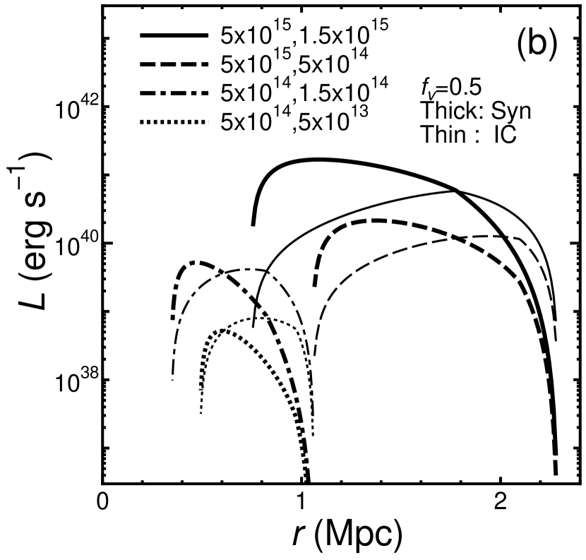
Figure 6: Same as Figure 1 but for (a) Model B1 (b) Model B2.

Figure 6 shows the nonthermal emission when $f_{v}=0.1$ and 0.5. The luminosities are small when $f_{v}$ is small. In particular, the synchrotron luminosity varies more than the inverse Compton luminosity. This is because the synchrotron luminosity is affected not only by the energy injection from fluid turbulence but also by magnetic fields. When $f_{v}$ or $v_{t}$ are small, the induced magnetic fields (eq. [60]) is also small. If $B<B_{\rm CMB}$, most of the nonthermal emission should be the inverse Compton emission rather than synchrotron emission (eqs. [58] and [59]). On the other hand, the results do not much depend on $f_{l}$.

The magnetic fields shown in Figure 2 are roughly consistent with the large values implied by Faraday rotation measurements (e.g., Lawler & Dennison, 1982; Kim et al., 1990; Goldshmidt & Rephaeli, 1993; Clarke, Kronberg, & Böhringer, 2001). However, the magnetic fields must be much smaller than the values implied by the Faraday rotation measurements if both nonthermal radio and hard X-ray emission are attributed to the same electron population with a power-law energy distribution without an upper cutoff (Fusco-Femiano et al., 1999, 2000). Thus, we also consider the case where the magnetic fields are small. Figure 7 shows the nonthermal emission when $b=0.001$. In this case, $B$ is about 30 times smaller than that in Figure 2. Although the synchrotron luminosity is not much different from that in Figure 1, the inverse Compton luminosity is much larger. This is because the total nonthermal luminosity becomes larger (eqs. [13] and [37]) and the fraction of Compton luminosity also becomes larger (eq. [59]). Since the maximum inverse Compton luminosity is relatively large ($\sim 10^{42-43}\rm\;erg\;s^{-1}$), the observations of both nonthermal radio and hard X-ray emission may be explained by this turbulence resonant acceleration model. If these small magnetic fields are correct, then the turbulent region must be different from the region where the Faraday rotation is measured.

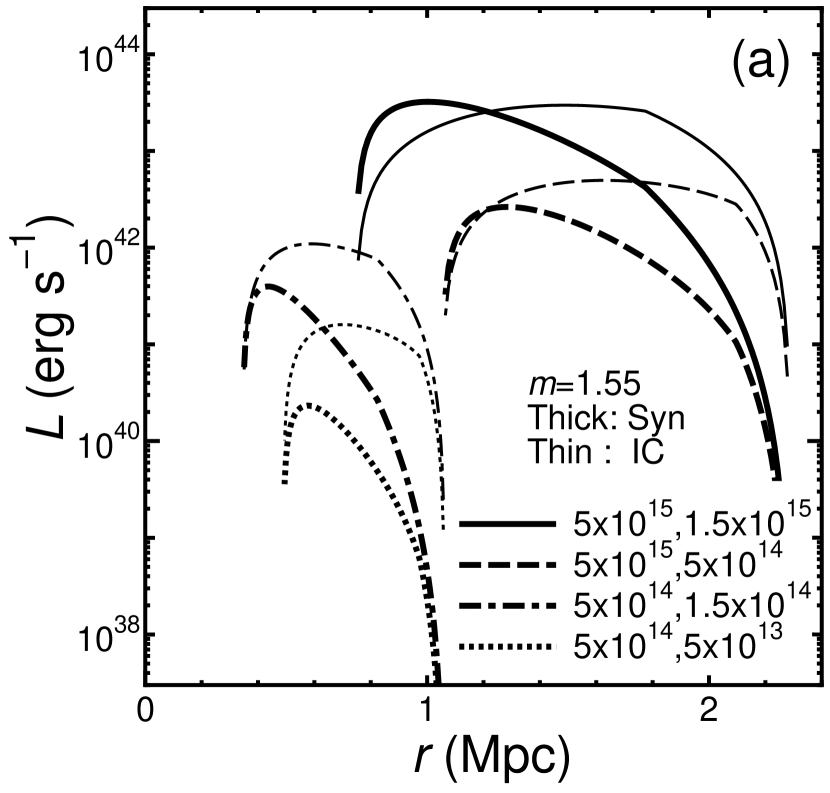
Figure 8: Same as Figure 1 but for (a) Model D1 (b) Model D2.

In §3.1, we assumed that the fluid turbulence follows the Kolmogorov law ($m=5/3$). However, for fully developed MHD turbulence, Iroshnikov (1963) and Kraichnan (1965) suggested that the spectral index should be $m=3/2$, although this is controversial (Goldreich & Sridhar, 1997). On the other hand, if turbulence has not had time to establish a Kolmogorov cascade, the index may be $m>5/3$. Thus, we discuss the $m$-dependence of the nonthermal emission. In Figure 8, we present the nonthermal emission when $m=1.55$ and 1.75. It shows that the emission is very sensitive to $m$. When $m=1.55$, the inverse Compton emission reaches $\sim 10^{43-44}\;\rm erg\;s^{-1}$, which is consistent with the observed hard X-ray luminosities (Fusco-Femiano et al., 1999, 2000) even though the magnetic field is strong ($b=1$). (Note that if we take $m=1.5$, the inverse Compton luminosity is much larger than the observed luminosities.) On the other hand, the synchrotron luminosity exceeds the observed values of $\lesssim 10^{41}\;\rm erg\;s^{-1}$. However, if the maximum energy of electrons is set by fluid viscosity at $\gamma\sim 10^{4}$ (eq. [40]), the observed synchrotron luminosity at $\sim 1$ GHz may be smaller than that shown in Figure 8 while the inverse Compton luminosity is almost the same (Brunetti et al., 2001a; Petrosian, 2001; Fujita & Sarazin, 2001). Thus, the model with $m<5/3$ can explain both the nonthermal radio and inverse Compton emission as a result of particle acceleration by turbulence.

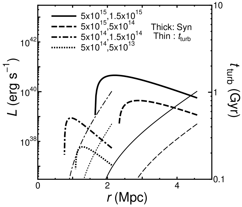
Figure 10: Same as Figure 5 but for Model E ($x_{i}=2$).

Although the possibility is small (Fujita et al., 2002), a smaller cluster may fall from the turnaround radius of a larger cluster ($x_{i}=2$). In this case, the smaller cluster has a large velocity near the center of the larger cluster compared to the case in §3.1. Figure 9 shows the nonthermal emission from the merging clusters. After the smaller cluster enters the virial radius of the larger cluster, it produces nonthermal emission. The maximum luminosities are not much different from those in Figure 1. Although the smaller cluster has a larger velocity, the radius is smaller owing to the larger ram-pressure. However, as shown in Figure 10, the time-scale of the fluid turbulence is small ($t_{\rm turb}\lesssim 10^{9}$ yr). This means that the turbulence cannot accelerate electrons at $\gamma\sim 10^{3}$ up to $\sim 10^{4}$, where the observed nonthermal emission is produced. Thus, the actual luminosities may even smaller than those shown in Figure 9. On the other hand, since the turbulent velocity is large ($\sim 10^{3}\rm\;km\;s^{-1}$; Figure 11), it would be easily observable by high spectral resolution X-ray detectors (e.g., Astro-E2).

3.3 Preheating

If the gas distribution of the small cluster has been flattened and the central gas density had been decreased by non-gravitational heating before cluster formation (preheating), the gas is more easily removed by the ram-pressure when the smaller cluster plunges into the larger cluster. Figure 9 shows how the nonthermal emission from merging clusters is affected by preheating. Compared with the case of no preheating (Figure 1), the maximum luminosities of the nonthermal emission is small especially when the mass of the smaller cluster is small. This is because preheating affects less massive clusters significantly and the gas is stripped earlier especially when the virial temperature of the smaller of the merging clusters approaches $T_{1}$ (eqs. [49] and [50]).

Radio observations have shown that the luminosity of diffuse radio emission from clusters is a steep function of cluster X-ray temperature or luminosity (Feretti, 2000; Liang et al., 2000). Since the sample of radio emission is small and less luminous radio clusters may not have been observed, this correlation may actually show that the maximum radio luminosity for a given X-ray temperature or luminosity is a steep function of cluster X-ray temperature or luminosity. This suggests that the steep correlation may apply only to clusters undergoing a major merger (small $M_{L,\rm vir}/M_{S,\rm vir}$).

Since the preheating reduces the nonthermal emission from less massive clusters, it may help to explain the observed steep correlation. We assume that $\min(M_{L,\rm vir}/M_{S,\rm vir})\sim 3$ and it does not depend on $M_{L,\rm vir}$. For the no preheating model (Figure 1), the synchrotron luminosity from merging clusters of $M_{L,\rm vir}=5\times 10^{14}M_{\sun}$ and $M_{S,\rm vir}=1.5\times 10^{14}M_{\sun}$ is about 50 times smaller than that from merging clusters of $M_{L,\rm vir}=5\times 10^{15}M_{\sun}$ and $M_{S,\rm vir}=1.5\times 10^{15}M_{\sun}$. If the temperature of the larger clusters are represented by $T_{\rm ICM}\propto M_{L,\rm vir}^{2/3}$ (e.g., Evrard, Metzler, & Navarro, 1996), the ratio of the temperature between the two cases is 4.6. Thus, the synchrotron luminosity from merging clusters roughly follows $L_{\rm syn}\propto T_{\rm ICM}^{2.6}$. Similarly, for the preheating model (Figure 9) we obtain $L_{\rm syn}\propto T_{\rm ICM}^{3.0}$. Since the virial temperature of the smaller cluster of $M_{S,\rm vir}=1.5\times 10^{14}M_{\sun}$ is $\sim T_{1}$, its merger with the larger cluster is significantly affected by the preheating. However, although preheating steepens the relation, the power-law index is still smaller than that observed ($\sim 6$; Feretti, 2000).

3.4 Turbulence Developed in the Whole Cluster

Numerical simulation done by Roettiger et al. (1999) showed that the fluid turbulence in ICM is also developed after a smaller cluster passes the center of a larger cluster. This turbulence is pumped by dark matter-driven oscillations in the gravitational potential; the merger-induced large scale bulk flows breakdown into turbulent gas motions. In this case, we expect the turbulence prevails on a cluster scale, and we can roughly estimate the nonthermal emission from the cluster. If we assume that $v_{t}=1000\rm\;km\>s^{-1}$, $l_{0}=1$ Mpc, $\rho_{\rm ICM}=7\times 10^{-28}\rm\>g\>cm^{-3}$, $T_{\rm ICM}=10^{8}$ K, $b=1$, and $m=5/3$, we obtain $L_{\rm syn}=8\times 10^{41}\rm\>erg\>s^{-1}$ and $L_{\rm IC}=1\times 10^{41}\rm\>erg\>s^{-1}$ using the model in §2. Thus, turbulence is strong enough to produce the observed synchrotron emission ($\sim 10^{41}\rm\>erg\>s^{-1}$), but cannot produce the observed hard X-ray emission ($\sim 10^{43-44}\rm\>erg\>s^{-1}$) as long as $m=5/3$ and the magnetic fields are strong ($b=1$). However, for the same parameters but with weak magnetic fields ($b=0.001$), we obtain $L_{\rm syn}=8\times 10^{41}\rm\>erg\>s^{-1}$ and $L_{\rm IC}=9\times 10^{43}\rm\>erg\>s^{-1}$. The luminosities are comparable to the observations. Observed central radio halos may be this kind of nonthermal emission from the whole cluster. The turbulent velocity, $v_{t}$, would be large enough to be detected by Astro-E2.

4 Conclusions

We have investigated nonthermal emission from electrons accelerated by resonant Alfvén waves in clusters of galaxies. We assume that the Alfvén waves are driven by fluid turbulence generated by cluster mergers. We find that the resonant Alfvén waves can accelerate electrons up to $\gamma\sim 10^{5}$; this value is limited by fluid viscosity. Our calculations show that the turbulent resonant acceleration can give enough energy to electrons to produce the observed diffuse radio emission from clusters if there is a pool of electrons of $\gamma\sim 10^{3}$ in clusters.. On the other hand, the observed hard X-ray emission from clusters is explained by the turbulent resonant acceleration only when magnetic fields are small ($\lesssim\mu G$) or the fluid turbulence spectrum is flatter than the Kolmogorov law. The fluid turbulence responsible for the particle acceleration would be observed by Astro-E2 in the regions where diffuse radio emission is observed. Although non-gravitational heating before cluster formation (preheating) makes the relation between radio luminosity and X-ray temperature steeper, our predicted relation is still flatter than the observed one.

Figure 1: Synchrotron (thick lines) and inverse Compton (thin lines) luminosities from merging clusters when the smaller cluster is at the distance $r$ from the center of the larger cluster. The solid, dashed, dot-dashed, and dotted lines correspond to $(M_{L,\rm vir},M_{S,\rm vir})=(5\times 10^{15},1.5\times 10^{15}),(5\times 10^{15},5\times 10^{14}),(5\times 10^{14},1.5\times 10^{14}),(5\times 10^{14},5\times 10^{13})\>M_{\sun}$, respectively.

Figure 2: Magnetic fields generated by fluid turbulence when the smaller cluster is at the distance $r$ from the center of the larger cluster with the mass of $M_{L,\rm vir}=5\times 10^{15}\>M_{\sun}$ (solid line) and $M_{L,\rm vir}=5\times 10^{14}\>M_{\sun}$ (dot-dashed line).

Figure 3: The velocity of fluid turbulence when the smaller cluster is at the distance $r$ from the center of the larger cluster with the mass of $M_{L,\rm vir}=5\times 10^{15}\>M_{\sun}$ (solid line) and $M_{L,\rm vir}=5\times 10^{14}\>M_{\sun}$ (dot-dashed line).

Figure 4: Spatial scale of nonthermal emission when the smaller cluster is at the distance $r$ from the center of the larger cluster. Notation is the same as Figure 1.

Figure 5: Thin lines are the time-scale for decay of fluid turbulence when the smaller cluster is at the distance $r$ from the center of the larger cluster. Thick lines are the synchrotron luminosities (same as those in Figure 1). Notation is the same as Figure 1.

Figure 7: Same as Figure 1 but for Model C.

Figure 9: Same as Figure 1 but for Model E ($x_{i}=2$).

Figure 11: Same as Figure 3 but for Model E ($x_{i}=2$).

Figure 12: Same as Figure 1 but for Model F (preheating).

Table 1: Model Parameters

Models	$f_{v}$	$b$	$m$	$x_{\rm i}$	Preheating
A	0.2	1	5/3	0.5	no
B1	0.1	1	5/3	0.5	no
B2	0.5	1	5/3	0.5	no
C	0.2	0.001	5/3	0.5	no
D1	0.2	1	1.55	0.5	no
D2	0.2	1	1.75	0.5	no
E	0.2	1	5/3	2	no
F	0.2	1	5/3	0.5	yes

References

- Arnaud & Evrard (1999) Arnaud, M., & Evrard, A. E. 1999, MNRAS, 305, 631
- Atoyan & Völk (2000) Atoyan, A. M., & Völk, H. J. 2000, ApJ, 535, 45
- Bahcall & Lubin (1994) Bahcall, N. A., & Lubin, L. M. 1994, ApJ, 426, 513
- Balogh et al. (1999) Balogh, M. L., Babul, A., & Patton, D. R. 1999, MNRAS, 307, 463
- Binney & Tremaine (1987) Binney, J., & Tremaine, S. 1987, Galactic Dynamics, (Princeton: Princeton Univ. Press), 452
- Blasi (2000) Blasi, P. 2000, ApJ, 532, L9
- Blasi (2001) Blasi, P. 2001, Astroparticle Physics, 15, 223
- Brunetti et al. (2001a) Brunetti, G., Setti, G., Feretti, L., & Giovannini, G. 2001, MNRAS, 320, 365
- Brunetti et al. (2001b) Brunetti, G., Setti, G., Feretti, L., & Giovannini, G. 2001, New Astronomy, 6, 1
- Bullock et al. (2001) Bullock, J. S., Kolatt, T. S., Sigad, Y., Somerville, R. S., Kravtsov, A. V., Klypin, A. A., Primack, J. R., & Dekel, A. 2001, MNRAS, 321, 559
- Buote (2001) Buote, D. A. 2001, ApJ, 553, L15
- Bykov et al. (2000) Bykov, A. M., Bloemen, H., & Uvarov, Y. A. 2000, A&A, 362, 886
- Cavaliere et al. (1998) Cavaliere, A., Menci, N., & Tozzi, P. 1998, ApJ, 501, 493
- Clarke, Kronberg, & Böhringer (2001) Clarke, T. E., Kronberg, P. P., & Böhringer, H. 2001, ApJ, 547, L111
- Colafrancesco & Blasi (1998) Colafrancesco, S., & Blasi, P. 1998, Astroparticle Physics, 9, 227
- David et al. (1996) David, L. P., Jones, C., & Forman, W. 1996, ApJ, 473, 692
- Dolag & Enßlin (2000) Dolag, K., & Enßlin, T. A. 2000, A&A, 362, 151
- Eilek (1979) Eilek, J. A. 1979, ApJ, 230, 373
- Eilek & Henriksen (1984) Eilek, J. A., & Henriksen, R. N. 1984, ApJ, 277, 820
- Enßlin et al. (1998) Enßlin, T. A., Biermann, P. L., Klein, U., & Kohle, S. 1998, A&A, 332, 395
- Enßlin & Brüggen (2002) Enßlin, T. A., & Brüggen, M. 2002, MNRAS, 331, 1011
- Enßlin & Gopal-Krishna (2001) Enßlin, T. A., & Gopal-Krishna 2001, A&A, 366, 26
- Ettori & Fabian (1999) Ettori, S., & Fabian, A. C. 1999, MNRAS, 305, 834
- Evrard et al. (1996) Evrard, A. E., Metzler, C. A., & Navarro, J. F. 1996, ApJ, 469, 494
- Feretti (2000) Feretti, L. 2000, preprint (astro-ph/0006379)
- Fujita (1998) Fujita, Y. 1998, ApJ, 509, 587
- Fujita (2001) Fujita, Y. 2001, ApJ, 550, 612
- Fujita & Sarazin (2001) Fujita, Y., & Sarazin, C. L. 2001, ApJ, 563, 660
- Fujita et al. (2002) Fujita, Y., Sarazin, C. L., Nagashima, M., & Yano, T. 2002, ApJ, in press (astro-ph/0205419)
- Fujita & Takahara (2000) Fujita, Y., & Takahara, F. 2000, ApJ, 536, 523
- Fusco-Femiano et al. (1999) Fusco-Femiano, R., Dal Fiume, D., Feretti, L., Giovannini, G., Grandi, P., Matt, G., Molendi, S., & Santangelo, A. 1999, ApJ, 513, L21
- Fusco-Femiano et al. (2000) Fusco-Femiano, R., et al., 2000, ApJ, 534, L7
- Fusco-Femiano et al. (2001) Fusco-Femiano, R., Dal Fiume, D., Orlandini, M., Brunetti, G., Feretti, L., & Giovannini, G. 2001, ApJ, 552, L97
- Gabici & Blasi (2002) Gabici, S., & Blasi, P. 2002, preprint (astro-ph/0207523)
- Giovannini et al. (1993) Giovannini, G., Feretti, L., Venturi, T., Kim, K.-T., & Kronberg, P. P. 1993, ApJ, 406, 399
- Giovannini et al. (1999) Giovannini, G., Tordi, M., & Feretti, L. 1999, New Astronomy, 4, 141
- Giovannini & Feretti (2000) Giovannini, G., & Feretti, L. 2000, New Astronomy, 5, 335
- Goldreich & Sridhar (1997) Goldreich, P., & Sridhar, S. 1997, ApJ, 485, 680
- Goldshmidt & Rephaeli (1993) Goldshmidt, O., & Rephaeli, Y. 1993, ApJ, 411, 518
- Gruber & Rephaeli (2002) Gruber, D. E., & Rephaeli, Y. 2002, ApJ, 565, 877
- Henriksen et al. (1982) Henriksen, R. N., Chan, K. L., & Bridle, A. H. 1982, ApJ, 257, 63
- Horner et al. (1999) Horner, D. J., Mushotzky, R. F., & Scharf, C. A. 1999, ApJ, 520, 78
- Ikebe et al. (1996) Ikebe, Y. et al. 1996, Nature, 379, 427
- Iroshnikov (1963) Iroshnikov, P. S. 1963, AZh, 40, 742
- Jaffe (1977) Jaffe, W. J. 1977, ApJ, 212, 1
- Kaastra et al. (1999) Kaastra, J. S., Lieu, R., Mittaz, J. P. D., Bleeker, J. A. M., Mewe, R., Colafrancesco, S., & Lockman, F. J. 1999, ApJ, 519, L119
- Kato (1968) Kato, S. 1968, PASJ, 20, 59
- Kempner & Sarazin (2001) Kempner, J. C., & Sarazin, C. L. 2001, ApJ, 548, 639
- Kim et al. (1990) Kim, K.-T., Kronberg, P. P., Dewdney, P. E., & Landecker, T. L. 1990, ApJ, 355, 29
- Kraichnan (1965) Kraichnan, R. H. 1965, Phys. Fluids, 8, 1385
- Kulsrud (1955) Kulsrud, R. M. 1955, ApJ, 121, 461
- Lawler & Dennison (1982) Lawler, J. M., & Dennison, B. 1982, ApJ, 252, 81
- Liang et al. (2000) Liang, H., Hunstead, R. W., Birkinshaw, M., & Andreani, P. 2000, ApJ, 544, 686
- Lighthill (1952) Lighthill, M. J. 1952, Proc. Roy. Soc. A. 211, 564
- Lloyd-Davies et al. (2000) Lloyd-Davies, E. J., Ponman, T. J., & Cannon, D. B. 2000, MNRAS, 315, 689
- Loewenstein (2000) Loewenstein, M. 2000, ApJ, 532, 17
- Markevitch et al. (2002) Markevitch, M., Gonzalez, A. H., David, L., Vikhlinin, A., Murray, S., Forman, W., Jones, C., & Tucker, W. 2002, ApJ, 567, L27
- Markevitch & Vikhlinin (2001) Markevitch, M., & Vikhlinin, A. 2001, ApJ, 563, 95
- Miniati et al. (2001) Miniati, F., Jones, T. W., Kang, H., & Ryu, D. 2001, ApJ, 562, 233
- Mohr et al. (1999) Mohr, J. J., Mathiesen, B., & Evrard, A. E. 1999, ApJ, 517, 627
- Navarro et al. (1996) Navarro, J. F., Frenk, C. S., & White, S. D. M. 1996, ApJ, 462, 563
- Navarro et al. (1997) Navarro, J. F., Frenk, C. S., & White, S. D. M. 1997, ApJ, 490, 493
- Ohno et al. (2002) Ohno, H., Takizawa, M., & Shibata, S. 2002, ApJ, in press (astro-ph/0206269)
- Ostrowski & Siemieniec-Oziȩbo (2002) Ostrowski, M., & Siemieniec-Oziȩbo, G. 2002, A&A, 386, 829
- Petrosian (2001) Petrosian, V. ; 2001, ApJ, 557, 560
- Ponman, Cannon, & Navarro (1999) Ponman, T. J., Cannon, D. B., & Navarro, J. F. 1999, Nature, 397, 135
- Ragot & Schlickeiser (1998) Ragot, B. R., & Schlickeiser, R. 1998, Astroparticle Physics, 9, 79
- Rephaeli et al. (1999) Rephaeli, Y., Gruber, D., & Blanco, P. 1999, ApJ, 511, L21
- Ricker & Sarazin (2001) Ricker, P. M., & Sarazin, C. L. 2001, ApJ, 561, 621
- Ritchie & Thomas (2002) Ritchie, B. W., & Thomas, P. A. 2002, MNRAS, 329, 675
- Roettiger et al. (1999) Roettiger, K., Stone, J. M., & Burns, J. O. 1999, ApJ, 518, 594
- Roland (1981) Roland, J. 1981, A&A, 93, 407
- Röttgering et al. (1994) Röttgering, H., Snellen, I., Miley, G., de Jong, J. P., Hanisch, R. J., & Perley, R. 1994, ApJ, 436, 654
- Röttgering et al. (1997) Röttgering, H. J. A., Wieringa, M. H., Hunstead, R. W., & Ekers, R. D. 1997, MNRAS, 290, 577
- Ruzmaikin et al. (1989) Ruzmaikin, A., Sokolov, D., & Shukurov, A. 1989, MNRAS, 241, 1
- Sarazin (1986) Sarazin, C. L. 1986, Rev. Mod. Phys., 58, 1
- Sarazin (1999) Sarazin, C. L. 1999, ApJ, 520, 529
- Sarazin (2002) Sarazin, C. L. 2002, in Merging Processes in Clusters of Galaxies, ed. Feretti, L., Gioia, I. M., & Giovannini, G. (Dordrecht: Kluwer), 1
- Schlickeiser & Miller (1998) Schlickeiser, R., & Miller, J. A. 1998, ApJ, 492, 352
- Schlickeiser et al. (1987) Schlickeiser, R., Sievers, A., & Thiemann, H. 1987, A&A, 182, 21
- Spitzer (1962) Spitzer, L., Jr. 1962, Physics of Fully Ionized Gases, 2nd Ed. (Interscience Publ: New York)
- Sun et al. (2002) Sun, M., Murray, S. S., Markevitch, M., & Vikhlinin, A. 2002, ApJ, 565, 867
- Takizawa & Mineshige (1998) Takizawa, M., & Mineshige, S. 1998, ApJ, 499, 82
- Takizawa & Naito (2000) Takizawa, M., & Naito, T. 2000, ApJ, 535, 586
- Tennekes & Lumley (1972) Tennekes, H., & Lumley, J. L. 1972, A First Course in Turbulence (Cambridge, MA: MIT Press)
- Totani & Kitayama (2000) Totani, T., & Kitayama, T. 2000, ApJ, 545, 572
- Vikhlinin et al. (2001) Vikhlinin, A., Markevitch, M., & Murray, S. S. 2001, ApJ, 551, 160
- Waxman & Loeb (2000) Waxman, E., & Loeb, A. 2000, ApJ, 545, L11
- Xue & Wu (2000) Xue, Y., & Wu, X. 2000, ApJ, 538, 65