Identifying Lenses with Small-Scale Structure. I. Cusp Lenses

Abstract

The inability of standard models to explain the flux ratios in many 4-image gravitational lens systems has been presented as evidence for significant small-scale structure in lens galaxies. That claim has generally relied on detailed lens modeling, so it is both model dependent and somewhat difficult to interpret. We present a more robust and generic method for identifying lenses with small-scale structure. For a close triplet of images created when the source lies near an ideal cusp catastrophe, the sum of the signed magnifications should exactly vanish, independent of any global properties of the lens potential. For realistic cusps, the magnification sum vanishes only approximately, but we show that it is possible to place strong upper bounds on the degree to which the magnification sum can deviate from zero. Lenses with flux ratio “anomalies,” or fluxes that significantly violate the upper bounds, can be said with high confidence to have structure in the lens potential on scales of the image separation or smaller. Five observed lenses have such flux ratio anomalies: B2045+265 has a strong anomaly at both radio and optical/near-IR wavelengths; B0712+472 has a strong anomaly at optical/near-IR wavelengths and a marginal anomaly at radio wavelengths; 1RXS J1131$-$1231 has a strong anomaly at optical wavelengths; RX J0911+0551 appears to have an anomaly at optical/near-IR wavelengths, although the conclusion in this particular lens is subject to uncertainties in the typical strength of octopole density perturbations in early-type galaxies; and finally, SDSS J0924+0219 has a strong anomaly at optical wavelengths. Interestingly, analysis of the cusp relation does not reveal a significant anomaly in B1422+231, even though this lens is known to be anomalous from detailed modeling. Methods that are more sophisticated (and less generic) than the cusp relation may therefore be necessary to uncover flux ratio anomalies in some systems. Although these flux ratio anomalies might represent either milli-lensing or micro-lensing, we cannot identify the cause of the anomalies using only broad-band flux ratios in individual lenses. Rather, the conclusion we can draw is that the lenses have significant structure in the lens potential on scales comparable to or smaller than the separation between the images. Additional arguments must be invoked to specify the nature of this small-scale structure.

1. Introduction

Gravitational lens modeling has had remarkable success handling increasingly precise measurements (e.g., Barkana et al. 1999; Patnaik et al. 1999; Trotter, Winn, & Hewitt 2000) and increasingly sophisticated datasets including Einstein ring images (Keeton et al. 2000; Kochanek, Keeton, & McLeod 2001) and/or stellar dynamical data (Romanowsky & Kochanek 1999; Koopmans & Treu 2002, 2003; Treu & Koopmans 2002, 2003; Koopmans et al. 2003b). Lens modeling has even clarified the properties of complex systems with more than one lens galaxy and/or more than one background source (Cohn et al. 2001; Rusin et al. 2001; Keeton & Winn 2003; Koopmans et al. 2003b). However, the notable success has largely been restricted to the number and configuration of lensed images. The flux ratios between the images, at least in lenses with four or more images, have long resisted explanation.

Until recently the persistent problem with flux ratios in 4-image lenses (e.g., Kent & Falco 1988; Falco, Lehár, & Shapiro 1997; Keeton, Kochanek, & Seljak 1997) received little attention, perhaps because the number of 4-image lenses was relatively small, and because it seemed possible to appeal to electromagnetic — non-gravitational — effects such as extinction by dust or scattering by hot gas. However, the number of lenses with apparently anomalous flux ratios is growing rapidly (e.g., Inada et al. 2003; Sluse et al. 2003; Wisotzki et al. 2003). Moreover, direct evidence suggests that electromagnetic effects, while present in some lenses, cannot explain most of the anomalies (Falco et al. 1999; Winn et al. 2001, 2002; Koopmans et al. 2003a). The problem with flux ratios therefore appears to be real.

It also turns out to have interesting and important implications for astrophysics and cosmology. When Mao & Schneider (1998) made the first systematic analysis of the flux ratio problem, they realized that the anomalies might be attributed to gravitational effects omitted from standard lens models, namely small-scale structure in the lens galaxy. The key insight was that since flux ratios are determined by second derivatives of the lens potential, they are much more sensitive to small-scale structure than the image positions (which are determined by first derivatives of the potential); so models that lack small-scale structure might successfully reproduce the image positions but fail to fit the flux ratios.

One possible source of small-scale structure is clumps of dark matter of mass $\sim\!10^{6}$–$10^{9}\,M_{\odot}$ left over from the hierarchical galaxy formation process in the Cold Dark Matter (CDM) paradigm (Metcalf & Madau 2001; Chiba 2002; Dalal & Kochanek 2002). This possibility has generated significant interest because it relates to current questions about the validity of CDM on small scales. The discrepancy between the predicted abundance of dark matter clumps and the observed abundance of dwarf galaxy satellites around the Milky Way has been interpreted as a fundamental problem with CDM (Klypin et al. 1999; Moore et al. 1999), which may signal a need for new physics for the dark matter (e.g., Spergel & Steinhardt 2000; Colin, Avila-Reese, & Valenzuela 2000; Hu, Barkana, & Gruzinov 2000). Alternately, the discrepancy may simply indicate poor understanding of the astrophysical processes that determine whether or not a clump of dark matter hosts a visible dwarf galaxy (Bullock, Kravtsov, & Weinberg 2000; Benson et al. 2002; Somerville 2002; Stoehr et al. 2002; Hayashi et al. 2002). If lens flux ratios can be used to probe dark matter clumps, that will provide the cleanest way to distinguish these two very different hypotheses, and more generally to resolve the controversy about whether CDM does or does not over-predict small-scale structure (e.g., Flores & Primack 1994; Moore 1994; Spergel & Steinhardt 2000; Debattista & Sellwood 2000; de Blok, McGaugh, & Rubin 2001; Keeton 2001a; van den Bosch & Swaters 2001; Weiner, Sellwood, & Williams 2001; de Blok & Bosma 2002; Kochanek 2003). Early results indicate that the statistics of flux ratio anomalies imply a clump population that agrees well with CDM predictions and validates cold dark matter (Dalal & Kochanek 2002; Kochanek & Dalal 2003), but the importance of the conclusion demands further study.

A second interesting possibility is that the small-scale structure implied by flux ratio anomalies is simply stars in the lens galaxy (Chang & Refsdal 1979; Irwin et al. 1989; Woźniak et al. 2000; Schechter & Wambsganss 2002). In this case, flux ratio anomalies offer a unique probe of the relative contributions of stars and dark matter to the surface mass density at the image positions (Schechter & Wambsganss 2002), which would be interesting because the amount of dark matter contained in the inner regions of elliptical galaxies is still not well known (e.g., Gerhard et al. 2001; Keeton 2001a; Borriello, Salucci, & Danese 2003; Rusin, Kochanek, & Keeton 2003b). Yet a third possibility is that the small-scale structure is not localized like dark matter clumps or stars, but is more global like small disk components in bulge-dominated systems, Fourier mode density fluctuations, tidal streams, etc. (e.g., Mao & Schneider 1998; Evans & Witt 2002; Quadri, Möller, & Natarajan 2003; Möller, Hewett, & Blain 2003). If this is the case, then lensing can be used to search for such structures whether they are traced by the luminous components of galaxies or not.

These three disparate applications all rest on a common foundation: the identification of lenses with flux ratio anomalies that indicate small-scale structure. That identification is most unambiguous when time variability (e.g., Woźniak et al. 2000; Schechter et al. 2003) or resolved spectra of the images (e.g., Moustakas & Metcalf 2003; Wisotzki et al. 2003) clearly indicate microlensing by stars in the lens galaxy, or when the resolved shapes of the images indicate structure on the scale of dark matter clumps (e.g., Metcalf 2002). Until such data become available for the majority of lenses, however, we need a method to identify anomalies using only broad-band flux ratios. Besides, such a method will be needed to select candidates for the expensive follow-up observations (monitoring, spectroscopy, or high-resolution imaging).

To date, the usual approach has been to use detailed lens modeling to interpret broad-band flux ratios and draw conclusions about, for example, the abundance of dark matter clumps (e.g., Dalal & Kochanek 2002; Metcalf & Zhao 2002; Kochanek & Dalal 2003). This approach is vulnerable to the criticism that the results depend on the sorts of lens potentials used in the modeling. The argument has two parts. First, many of the commonly used families of lens potentials implicitly possess global symmetries, which lead to invariant magnification relations that are “global” in the sense that they involve all four images (Dalal 1998; Witt & Mao 2000; Dalal & Rabin 2001; Hunter & Evans 2001; Evans & Hunter 2002). If a fit is poor because the data fail to satisfy these relations, that does not automatically constitute a flux ratio anomaly; it may simply indicate that the assumed relations are too restrictive, and that small, unremarkable deviations from the assumed symmetries are needed. The conceptual difficulty here is that one is trying to use global relations to draw conclusions about structure on smaller, more local scales. The second part of the argument is that there is a large difference in scale between the image separations ($\sim\!0\farcs 2$–$2\arcsec$) and the scales relevant for dark matter clumps ($\sim\!10^{-3}\arcsec$) or stars ($\sim\!10^{-6}\arcsec$). If the flux ratio anomalies are in fact due to structures that are intermediate between these scales, then they may not necessarily imply the presence of dark matter clumps or stars (Evans & Witt 2002; Quadri et al. 2003; Möller et al. 2003).

To address the first part of the criticism, we seek a method of identifying flux ratio anomalies that is local rather than global, i.e., a method that is sensitive only to structures smaller than the scales probed by the image positions. Fortunately, one can do this by appealing to simple, generic relations between the image magnifications that should be satisfied for images in “fold” or “cusp” configurations (defined in §2). The magnification relations are derived from local properties of the lens mapping and are in principle independent of the global mass model. They can be violated only if there is significant structure in the lens potential in scales smaller than the separations between the images (see Mao & Schneider 1998). In practice, however, the situation is complicated by the fact that the caustics in real lens systems only approximate ideal folds and cusps in some low-order expansion of the potential near the critical point; higher-order terms introduce deviations from the fold and cusp geometries. Real lenses therefore need to obey the ideal magnification relations only approximately. Because the accuracy with which the relations should hold depends on the distance of the images from the critical point and on properties of the lens potential, it is not straightforward to judge a priori the significance of an apparent violation.

Our goal is to understand the magnification relations in realistic lens potentials and to determine how well they can be used to identify flux ratio anomalies. In this paper we focus on cusp configurations, because as the highest order stable singularities in lensing maps (see Schneider, Ehlers, & Falco 1992; Petters, Levine, & Wambsganss 2001) cusps are amenable to analytic study, and cusp configurations are easy to identify. We will address fold configurations in subsequent work. We study the degree to which the ideal cusp relation can be violated due to various properties of the lens potential: the radial density profile, ellipticity, and multipole density perturbations of the lens galaxy, and the external tidal shear from the lens environment. Using both analytic and numerical methods we derive upper bounds on the deviation from the ideal cusp relation for realistic lens potentials that lack significant small-scale structure. We then argue that finding larger deviations in observed lenses robustly reveals flux ratio anomalies and indicates the presence of some sort of small-scale structure.

We assert that, even though we adopt specific families of lens potentials, our analysis is more general than explicit modeling. One reason is that we have a better distinction between global and local properties of the lens potential. For example, a global $m=1$ mode (i.e., non-reflection symmetry) would affect conclusions about anomalies in direct modeling, but not in our analysis. A second reason is that we consider quite general forms for the lens potential and take care to understand which generic features affect the cusp relation. A third point is that our results are less modeling dependent, less subject to the intricacies of fitting data and using minimization routines. A fourth advantage of our analysis is that, rather than simply showing that standard models fail to fit a lens, it clearly diagnoses why. We believe that these benefits go a long way toward establishing that small-scale structure in lens galaxies is real and can be understood.

We must address a question that is purely semantic but nevertheless important: Where do we draw the line between a normal “smooth” lens potential and “small-scale structure”? Taking a pragmatic approach, we consider “smooth” to mean any features known to be common in (early-type) galaxies: certain radial density profiles, reasonable ellipticities, small octopole modes representing “disky” or “boxy” isophotes, and reasonable external shears. We consider “small-scale structure” to be anything whose presence in early-type galaxies would be notable. This can include stars — although stars are obviously abundant in galaxies, detecting the gravitational effects of individual stars is still interesting — and dark matter clumps, which seem to have generated the most interest. But it may also include tidal streams, massive or offset disk components (see Quadri et al. 2003; Möller et al. 2003), large-amplitude multipole density fluctuations (see Evans & Witt 2003), etc. We emphasize that our analysis, or indeed any analysis that considers only the image positions and broad-band flux ratios in individual lenses, cannot distinguish between these types of small-scale structure. The most general conclusion we can draw from flux ratio anomalies is that the lens potential contains structure on scales comparable to or smaller than the separation between the images. Further data and analysis is required to determine the nature of the small-scale structure (e.g., Woźniak et al. 2000; Metcalf 2002; Kochanek & Dalal 2003; Moustakas & Metcalf 2003; Schechter et al. 2003; Wisotzki et al. 2003).

The layout of the paper is as follows. We begin in §2 by reviewing quadruple imaging and introducing a way to characterize 4-image configurations quantitatively. (In this paper we consider only 4-image lenses.) In §3 we discuss cusp image configurations and present the generic, universal relation that should be obeyed by the image magnifications for sources near an ideal cusp. We then test this ideal relation, first using analytic results for simple lens potentials (§4), and then with Monte Carlo simulations of realistic lens populations (§5). In §6 we apply the cusp relation to observed lenses, using violations of the relation to identify lenses that require small-scale structure. We offer our conclusions in §7. Several appendices present supporting technical material. In Appendix A we derive the universal relations between the image positions and magnifications for sources near an ideal cusp. In Appendix B we obtain exact analytic solutions of the lens equation for two families of lens potentials, which can be used to obtain exact analytic expressions for the realistic cusp relation.

2. Characterizing 4-Image Lenses

Nineteen quadruply-imaged lens systems have appeared in the literature, and they are listed in Table 1. This count includes only systems that have exactly four images of a given source, and where the images appear point-like at some wavelength. It includes the 10-image system B1933+503, which is complex only because there are three distinct sources; none of the sources has an image multiplicity larger than four (Sykes et al. 1998). By contrast, it excludes PMN J0134$-$0931 and B1359+154 because they have multiplicities larger than four due to the presence of multiple lens galaxies (Rusin et al. 2001; Keeton & Winn 2003; Winn et al. 2003). One other lens, 0047$-$2808, is almost certainly quadruply-imaged as well (Warren et al. 1996, 1999; Koopmans & Treu 2003), but its lack of point-like images makes it difficult to analyze with the usual techniques used for point-like systems.

Mathematically, quadruple imaging can be described in terms of the critical curves and caustics of the lens potential. (See the monographs by Schneider et al. 1992 and Petters et al. 2001 for thorough reviews of lens theory.) Critical curves are curves in the image plane where the lensing magnification is formally infinite, and caustics are the corresponding curves in the light source plane. The properties of these curves can be studied with catastrophe theory; for our purpose the important result is that the astroid-shaped caustic that is associated with quadruple imaging has a generic shape that leads to three generic configurations of 4-image lenses (see Figure 1). Sources near a cusp in the caustic produce “cusp” configurations with three of the images lying close together on one side of the lens galaxy. Source near the caustic but not near a cusp produce “fold” configurations with two of the images lying close together. Sources not close to the caustic produce relatively symmetric “cross” configurations.

Figure 1.— The three basic configurations of 4-image lenses: fold (top), cusp (middle), and cross (bottom). In each panel, the figure on the left shows the caustics and source position in the light source plane, while the figure on the right show the critical curves and image positions in the image plane.

Although it may seem easy to label an observed lens as a fold, cusp, or cross, the categories actually blend together so it is important to develop a more quantitative way to characterize image configurations. To quantify a triplet of images (as in a cusp configuration), let $d$ be the maximum separation between the three images, and let $\theta$ be the opening angle of the polygon spanned by the three images, measured from the position of the lens galaxy. Each 4-image lens has four distinct triplets and hence four values of $\theta$ and $d$. We can identify image triplets associated with cusps as those where $\theta$ and/or $d$ is small (see Figure 2). Even though there is no rigorous definition of when $\theta$ and $d$ are “small” enough to indicate a cusp configuration, we shall see below that these are useful quantities for characterizing the range of image configurations.

Figure 2.— Sample image triplets for the image configurations from Figure 1, together with the values of the opening angle $\theta$ and the separation $d$ (in units of the Einstein radius of the lens). The star shows the position of the lens galaxy in each system.

3. Universal Magnification Relation for Cusps

In this section we briefly review the lensing of a source close to and inside an ideal cusp and present the magnification relation used in our analysis. Appendix A discusses lensing near a cusp in considerably more detail, and presents additional position and magnification relations for cusp images. This analysis applies to ordinary cusps; it may not be valid for so-called ramphoid cusps (or cusps of the second kind), but such cusps have not been observed and are expected to be rare in lensing situations of astrophysical interest (see Petters & Wicklin 1995; Oguri et al. 2003).

In the vicinity of a cusp, the lens equation relating the source position $u$ to the image position $\theta$ can be written to third order in $\theta$ as a polynomial mapping,

$$u_{1}=c\ \theta_{1}\ +\ \frac{b}{2}\ \theta^{2}_{2}\,,\qquad u_{2}=b\ \theta_{1}\ \theta_{2}+a\ \theta_{2}^{3}\,.$$ (1)

The coordinates $u$ and $\theta$ are local orthogonal coordinates that are related to the global coordinates ${\bf y}$ and ${\bf x}$ of the lens system by ${\mbox{\boldmath$u$}}\equiv{\rm M}{\bf y}$ and ${\mbox{\boldmath$\theta$}}\equiv{\rm M}{\bf x}$, where the transformation matrix ${\rm M}$ depends on the lens potential. For the simple cases that we study in §4 and Appendix B, ${\rm M}$ is the identity matrix and the $\theta$ and $u$ coordinate systems are simply the ${\bf x}$ and ${\bf y}$ coordinate systems translated so the cusp point is at the origin. The constant coefficients $a$, $b$, and $c$ are given by derivatives of the potential at the critical point (see eq. A6 in Appendix A).

Solving for $\theta_{1}$ in the left-hand side of eq. (1) and substituting into the right-hand side, one obtains a cubic equation for $\theta_{2}$ that depends on $a$, $b$, $c$, and the source position $u$. Inside the caustic, there are three real solutions to this cubic equation, and thus three images of the source. It is possible to derive six independent relations between the positions and magnifications of these images. Unfortunately, only one of these relations can be recast to depend only on directly observable properties: the well-known magnification sum rule (Schneider & Weiss 1992; Zakharov 1995; Petters et al. 2001, p. 339),

$$\mu_{1}+\mu_{2}+\mu_{3}=0\,,$$ (2)

where the $\mu_{i}$ are the signed magnifications of the three images. The other relations depend on properties that are not directly observable, such as the position of the source or the mapping coefficients $a$, $b$, and $c$.

4. The Cusp Relation in Simple Lens Potentials

The derivation of the ideal cusp relation eq. (2) relies on the assumption that the lensing map has the polynomial form of eq. (1). Since this form is a truncated Taylor series expansion near the cusp point, we should expect the cusp relation to be exact only for sources asymptotically close to the cusp. In this section we begin to quantify the deviation from the ideal cusp relation that arise from the higher order terms in the lensing map, using simple examples to illustrate the effects of the radial profile, ellipticity, shear, and multipole perturbations of the lens potential.

The magnifications appearing in the cusp relation are not directly observable, but we can follow Mao & Schneider (1998) and divide out the unknown source flux by defining the dimensionless quantity

$$R_{\rm cusp}\equiv\frac{|\mu_{1}+\mu_{2}+\mu_{3}|}{|\mu_{1}|+|\mu_{2}|+|\mu_{3}|}=\frac{|F_{1}+F_{2}+F_{3}|}{|F_{1}|+|F_{2}|+|F_{3}|}\ ,$$ (3)

where the $\mu_{i}$ are the magnifications and the $F_{i}$ the observed fluxes, both with signs indicating the image parities. The parities can be determined unambiguously because in any triplet of adjacent images, the two outer images have the same parity while the middle image has the opposite parity (see Schneider et al. 1992; Petters et al. 2001). The ideal cusp relation has the form $R_{\rm cusp}=0$.

Note that we have defined $R_{\rm cusp}$ to be non-negative. Several recent studies (Schechter & Wambsganss 2002; Keeton 2003; Kochanek & Dalal 2003) have pointed out that small-scale structure tends to suppress negative-parity images more often than it amplifies positive-parity images, while global perturbations generally do not distinguish between images with different parities. In an ensemble of lenses with flux ratio anomalies, skewness in the signed $R_{\rm cusp}$ distribution may therefore distinguish local from global perturbations. However, the statistical nature of this argument precludes its use in individual lenses. Since we seek a method of identifying anomalies in individual lenses, we consider only the unsigned quantity.

We first study the cusp relation analytically using two families of lens potentials where it is possible to obtain exact solutions of the lens equation. In one family, the galaxy is assumed to be spherical but is allowed to have a general power law surface density profile $\Sigma\propto r^{\alpha-2}$ and to have an external shear $\gamma$. In the other family, the galaxy is assumed to have an “isothermal” profile $\Sigma\propto r^{-1}$ but is allowed to have a complex angular structure, including shear; we specifically consider an ellipsoidal galaxy perturbed by multipole density fluctuations. Appendix B describes the two families of lens potentials in detail and gives solutions for the positions and magnifications of images corresponding to sources on a symmetry axis of the lens potential.

Figure 3.— The cusp relation residual $R_{\rm cusp}$ as a function of the opening angle $\theta$ and the separation $d$ of an image triplet, plotted for various lens potentials using the analytic solutions to the lens equation for sources on the major axis of the potential. In panel (c), $\gamma>0$ ($\gamma<0$) represents a shear aligned with (orthogonal to) the major axis of the galaxy.

Figure 3 shows $R_{\rm cusp}$ versus the opening angle $\theta$ and separation $d$ of an image triplet, for various potentials with different radial profiles, ellipticities, and shears. In general, $R_{\rm cusp}$ is small when $\theta$ and $d$ are small (indicating that the source is very near a cusp), and grows as $\theta$ and $d$ grow (indicating that the source is moving farther from the cusp). The analytic results allow us to understand how departures from the ideal cusp relation depend on properties of the lens potential. We see that radical changes in the radial profile of the lens potential — from $\alpha=1$ (isothermal) to $\alpha=0$ (point mass) — have a negligible effect on the cusp relation. By contrast, moderate changes in the ellipticity and shear can affect the cusp relation by tens of percent. The fact that the cusp relation is quite sensitive to ellipticity, moderately sensitive to shear, and not very sensitive to the radial profile makes sense: reasonable changes in the angular structure of the potential ($e$ and $\gamma$) can affect nearby images quite differently, while reasonable changes in the radial profile cannot. Incidentally, we note that when considering fixed ellipticity and shear amplitudes, $R_{\rm cusp}$ can be larger when the two are orthogonal than when they are aligned.

Figure 4.— Effects of multipole perturbations on the cusp relation, for isothermal ellipsoid lens potentials with $e=0.3$ and $\gamma=0$. The heavy dashed curves all show a reference case with no multipole modes. (a) The effects of $m=4$ density fluctuations with amplitude $a_{4}=(\pm 0.01,\pm 0.02,\pm 0.03)$ indicated by increasing line thickness. Solid (dotted) curves correspond to $a_{4}>0$ ($a_{4}<0$). The sources lie on the major axis of the lens potential. (b) Similar to (a), but for sources on the minor axis of the potential (c) The effects of multipole perturbations of different orders, all with amplitude $a_{m}=0.02$. Lines of increasing thickness and alternating type indicate $m=(6,8,10,12,14,16)$. The cross on each curve marks the point with $\theta=640\arcdeg/m$. The sources lie on the major axis of the lens potential.

The effects of multipole density perturbations are shown in Figure 4, for lens potentials with an “isothermal” ($\alpha=1$) radial profile. Multipole modes with $m=3$ or 4 and amplitudes of a few percent are common in the isophotes of observed early-type galaxies (Bender et al. 1989; Saglia et al. 1993; Rest et al. 2001) and in the isodensity contours of simulated galaxy merger remnants (Heyl, Hernquist, & Spergel 1994; Naab & Burkert 2003; Burkert & Naab 2003); in particular, $m=4$ modes with amplitudes $a_{4}>0$ can represent small disk-like components in bulge-dominated galaxies, which are not unusual (Kelson et al. 2000; Tran et al. 2003). Such modes might have a significant effect on the magnifications of lensed images (Evans & Witt 2002; Möller et al. 2003). We find that $m=4$ modes do not significantly increase $R_{\rm cusp}$ for cusp triplets with $\theta\lesssim 90\arcdeg$ when the source is on the major axis of the lens potential (Figure 4a). However, they can create remarkably large values of $R_{\rm cusp}$ even for small $\theta$ when the source is on the minor axis (Figure 4b). At fixed amplitude, higher order modes produce progressively larger values of $R_{\rm cusp}$ at smaller angles (Figure 4c). The position of the peak in the $R_{\rm cusp}$ curve for different values of $m$ can be approximated as $\theta_{\rm peak}\sim 640\arcdeg/m$. This result describes our fiducial case with $e=0.3$ and $a_{m}=0.02$; varying $e$ and $a_{4}$ has a small ($\lesssim$5%) effect on the position of the peak, but a large effect on the amplitude of the peak. Thus, we can say as a rule of thumb that image triplets with angle $\theta$ are significantly affected only by modes with $m\gtrsim 640\arcdeg/\theta$. We conclude that it is important to consider multipole effects in the cusp relation analysis. But as it is not clear that real galaxies have percent-level perturbations in modes beyond $m\approx 4$, it is equally important to hold the perturbations to reasonable levels.

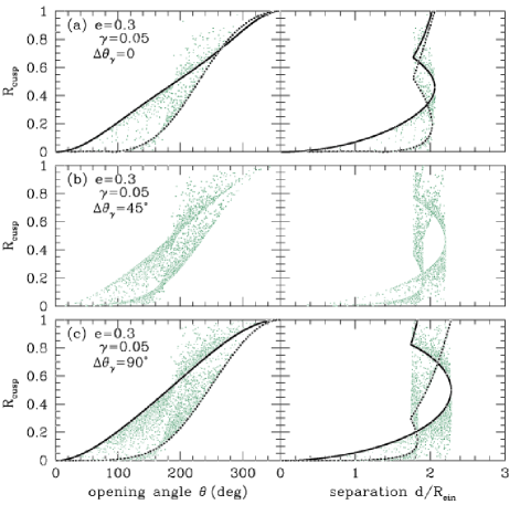
Figure 5.— $R_{\rm cusp}$ versus $\theta$ and $d$, for various values of the ellipticity and shear and the angle $\Delta\theta_{\gamma}$ between them. The points show results for Monte Carlo simulations of random source positions. The heavy curves show the analytic results for on-axis sources, where solid (dotted) curves indicate the major (minor) axis of the lens potential. Analytic results are available only for $\Delta\theta_{\gamma}=0$ and $90\arcdeg$.

So far we have studied only sources lying on a symmetry axis of the lens potential. For the more general case we turn to Monte Carlo simulations. We pick random source positions and solve the lens equation (using the algorithm and software by Keeton 2001b) to generate a catalog of mock lenses. We compute $\theta$, $d$, and $R_{\rm cusp}$ for each triplet in each 4-image lens, and then plot $R_{\rm cusp}$ versus $\theta$ or $d$ for all triplets. Figure 5 shows sample results for isothermal ellipsoid galaxies with shear. The most important result is that over the region of interest for the cusp relation ($\theta\lesssim 180\arcdeg$ and $d/R_{\rm ein}\lesssim 1.7$) there is a firm upper envelope on the values of $R_{\rm cusp}$. In fact there are two envelopes: one each for major and minor axis cusps. Moreover, in lenses with reflection symmetry the envelope corresponds to sources on the symmetry axis. To understand this result, in Appendix B.1 we prove that $R_{\rm cusp}$ is a local maximum on the symmetry axis of an isothermal sphere plus shear. Messy algebra hinders a rigorous analysis of other potentials, but intuition and the Monte Carlo simulations suggest that the result is generally true. In other words, the analytic results for on-axis sources provide a simple and important upper bound on $R_{\rm cusp}$.

To summarize, the ideal cusp relation breaks down for sources a small but finite distance from the cusp, but in a way that can be understood and quantified. The realistic cusp relation is mainly sensitive to the angular structure of the lens potential, not the radial profile. The important quantities are the ellipticity, shear, and strength of multipole density fluctuations. For the subset of cusps that possess a symmetry axis, sources on that axis provide a strict upper bound on $R_{\rm cusp}$ over the interesting range of $\theta$ and $d$ that can often be derived analytically.

5. The Cusp Relation in Realistic Lens Populations

If we knew the ellipticity, shear, and multipole perturbations for individual observed lenses, we could use the previous analysis to compute how much $R_{\rm cusp}$ can deviate from zero for smooth potentials and then conclude that larger values represent flux ratio anomalies. Unfortunately, the three key quantities are not directly observable. The ellipticity and multipole perturbations of the mass need not be the same as those of the light (e.g., Keeton, Kochanek & Falco 1998), and in any case the shear cannot be directly observed. The three quantities could be constrained with lens models, but we seek to avoid explicit modeling to the extent possible. Instead, our approach is to adopt observationally-motivated priors on the ellipticity, multipole perturbations, and shear, and use Monte Carlo simulations to obtain a sample of realistic lens potentials and derive probability distributions for $R_{\rm cusp}$. In this section we describe the priors (§5.1) and methods (§5.2) for the simulations.

5.1. Input distributions

We consider only early-type galaxies, because they are expected to dominate the lensing optical depth due to their large average mass (e.g., Turner, Ostriker, & Gott 1984; Fukugita & Turner 1991). Indeed, $\sim$80–90% of observed lens galaxies have properties consistent with being massive ellipticals (Keeton et al. 1998; Kochanek et al. 2000; Rusin et al. 2003a). The distinction between ellipticals and spirals is important, because disk-dominated galaxies that are viewed close to edge-on can produce cusp configurations that deviate significantly from the cusp relation (Keeton & Kochanek 1998). Several of the lenses for which we identify flux ratio anomalies are confirmed ellipticals, and none of them have properties suggesting that they are spirals (Impey et al. 1996; Burud et al. 1998; Fassnacht et al. 1999; Jackson et al. 2000; Inada et al. 2003; Sluse et al. 2003; Rusin et al. 2003a).

We allow the simulated galaxies to have ellipticity and also octopole ($m=4$) perturbations, with distributions drawn from observations of isophote shapes in early-type galaxies. Even if the shapes of the mass and light distributions are not correlated on a case-by-case basis, it seems likely that their distributions are similar (see Rusin & Tegmark 2001 for a discussion). Indeed, the distribution of isodensity contour shapes in simulated merger remnants is very similar to the observed distribution of isophote shapes (Heyl et al. 1994; Naab & Burkert 2003; Burkert & Naab 2003). Multipole perturbations beyond $m\geq 5$ have generally not been reported, but it is likely that they must have relatively low amplitudes to be compatible with observations. Lower-order $m=3$ modes have been reported with amplitudes comparable to $m=4$ modes (e.g., Rest et al. 2001), but we do not consider them here because they are not reported in the samples we use, and because at fixed amplitude higher-order modes produce larger deviations in the cusp relation (see Figure 4). Our approach is formally equivalent to studies that explicitly include a disk-like mass component (e.g., Möller et al. 2003), since small disks can be treated as $m=4$ multipole perturbations. We use only isothermal galaxies, because the radial profile of the lens galaxy does not significantly affect the cusp relation. The galaxy mass is unimportant, because it simply sets a length scale (the Einstein radius) that can be scaled out by using the dimensionless separation $d/R_{\rm ein}$.

We use ellipticity and octopole distributions from three different samples. Jørgensen et al. (1995) report ellipticities for 379 E and S0 galaxies in 11 clusters, including Coma. Their ellipticity distribution has mean ${\bar{e}}=0.31$ and dispersion $\sigma_{e}=0.18$. Since the Jørgensen et al. sample does not include octopole amplitudes, we consider two smaller samples that do. Bender et al. (1989) report ellipticities and octopoles for 87 nearby, bright elliptical galaxies. Their ellipticity distribution has ${\bar{e}}=0.28$ and $\sigma_{e}=0.15$, while their octopole distribution has mean ${\bar{a}}_{4}=0.003$ and dispersion $\sigma_{a_{4}}=0.011$. Finally, Saglia et al. (1993) report ellipticities and octopole amplitudes for 54 ellipticals in Coma, with ${\bar{e}}=0.30$ and $\sigma_{e}=0.16$, and ${\bar{a}}_{4}=0.014$ and $\sigma_{a_{4}}=0.015$. Compared to the Bender et al. sample, the Saglia et al. sample has a higher incidence of galaxies with strong disky perturbations ($a_{4}>0$). Considering all three samples allows us to examine whether our conclusions depend systematically on the input $(e,a_{4})$ distributions (although we note that since the Jørgensen et al. and Saglia et al. samples both include galaxies in Coma they are not fully independent). Figure 6 shows the different samples and suggests that $e$ and $a_{4}$ are correlated such that highly elliptical galaxies tend to have significant disky perturbations. Our analysis includes this correlation explicitly by using the observed joint distribution of $e$ and $a_{4}$.

Figure 6.— The main panel shows the $e$ and $a_{4}$ values for the galaxies in the Bender et al. (1989) and Saglia et al. (1993) samples. Galaxies with $a_{4}>0$ ($a_{4}<0$) have disky (boxy) isophotes. The right panel shows the histograms of $a_{4}$. The top panel shows histograms of $e$ for these samples and also the Jørgensen et al. (1995) sample.

For the shear amplitude we adopt a lognormal distribution with median $\gamma=0.05$ and dispersion $\sigma_{\gamma}=0.2$ dex. This is consistent with the distribution of shears expected from the environments of early-type galaxies, as estimated from $N$-body and semi-analytic simulations of galaxy formation (Holder & Schechter 2003). It is broadly consistent with the empirical distribution of shears required to fit observed lenses, when selection biases related to the lensing cross section and magnification bias are taken into account (see Holder & Schechter 2003). The mean shear is also consistent with the typical value needed to explain misalignments between the light and mass in observed lenses (Kochanek 2002). We assume random shear orientations.

5.2. Simulation methods

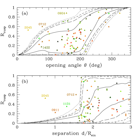
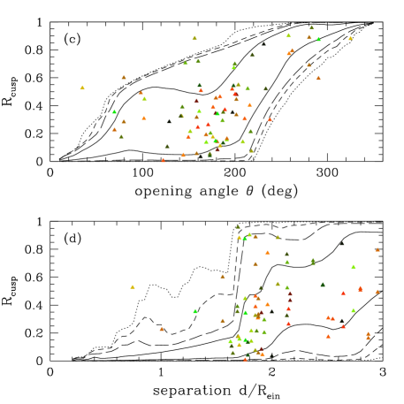
Figure 7.— The curves show contours of constant conditional probability $p(R_{\rm cusp}|\theta)$ (top) and $p(R_{\rm cusp}|d)$ (bottom), from Monte Carlo simulations using the Jørgensen et al. input data (left) or the Bender et al. input data (right). The contours are drawn at the 68% (solid), 95% (long-dashed), 99% (dashed), and 99.9% (dotted) confidence levels. The points show the observed values of $R_{\rm cusp}$ for the known 4-image lenses. B0712+472 appears twice; the lower value of $R_{\rm cusp}$ corresponds to the radio data, while the higher value (labeled) corresponds to the optical/near-IR data (see text).

We use each input distribution to run a large Monte Carlo simulation containing $\sim\!10^{6}$ 4-image lenses. With the Jørgensen et al. sample we draw 2000 ellipticities from the observed ellipticity distribution and give each a random shear. With the Bender et al. and Saglia et al. samples we use only the observed $(e,a_{4})$ pairs to make sure we include the apparent correlation between the two quantities, but we use each pair with 100 different random shears; thus we consider 8700 and 5400 lens potentials for the Bender et al. and Saglia et al. samples, respectively, but we need to remember that these represent only 87 and 54 different ellipticity and octopole measurements. For each potential, we pick random sources with a uniform density of $\sim\!10^{3}\,R_{\rm ein}^{-2}$ in the source plane and solve the lens equation using the algorithm and software by Keeton (2001b). We have verified that our results are not sensitive to the number of shears and density of sources used.

To understand how our mock lenses compare to observed samples it is important to consider two selection effects. First, the cross section for 4-image lenses is very sensitive to ellipticity and shear, but our uniform sampling of the source plane ensures that each lens potential is automatically weighted by the correct cross section. Second, magnification bias can favor lenses with higher amplifications. While this effect is important when comparing 4-image lenses to 2-image lenses (e.g., Keeton et al. 1997; Rusin & Tegmark 2001), it is much less important when comparing different 4-image lenses against each other. If anything, it would favor the sources very near a cusp or fold that yield extremely magnified lenses that best satisfy the cusp/fold relations, giving more weight to lenses with smaller deviations from the ideal relations. We therefore neglect magnification bias and believe that this is a conservative approach.

We compute $\theta$, $d$, and $R_{\rm cusp}$ for each image triplet in each mock 4-image lens, and use this ensemble to determine the conditional probability distributions $p(R_{\rm cusp}|\theta)$, $p(R_{\rm cusp}|d)$, and $p(R_{\rm cusp}|d,\theta)$ — the probability of having a particular value of $R_{\rm cusp}$ given $\theta$, $d$, or both. For example, Figure 7 shows curves of constant conditional probability $p(R_{\rm cusp}|\theta)$ and $p(R_{\rm cusp}|d)$ versus $\theta$ and $d$. This figure is basically a modified version of Figure 5 where we have averaged over appropriate ellipticity, octopole, and shear distributions. It is interpreted as saying that 68% of triplets in our sample of mock lenses lie in the region between the solid curves, 99% lie between the dashed curves, and so forth. To the extent that our simulations encompass the range of ellipticities, octopoles, and shears in real populations of early-type galaxies, we can conclude that any points lying outside the contours represent flux ratios that are inconsistent with smooth lens potentials.

6. Application to Observed Lenses

We can now use our theoretical analysis to evaluate observed lenses, seeking to identify systems that violate the cusp relation and therefore have anomalous flux ratios. We first summarize the data (§6.1) and then present our results (§6.2).

6.1. Data

The data for the nineteen published 4-image lenses are given in Table 1. Only five of the lenses are thought to have cusp configurations, but we can still apply the cusp relation analysis to all of them to see what we learn. In the table we list the four different image triplets for each lens, with the opening angle $\theta$, the image separation $d$, and the observed value of $R_{\rm cusp}$ for each. If the lens galaxy position is known, the angle $\theta$ is fully determined by the data; if not, we estimate $\theta$ using the galaxy position estimated from lens models, which is a fairly model-independent prediction. The separation $d$ is determined directly from the data. To normalize it we need the Einstein radius $R_{\rm ein}$, which must be derived from a lens model but is insensitive to the assumed model; different models generally yield the same Einstein radius with systematic uncertainties of just a few percent (Cohn et al. 2001; Rusin et al. 2003b).

When we measure $R_{\rm cusp}$ we need to consider systematic uncertainties due to effects like source variability and the lens time delay, scatter broadening (at radio wavelengths), and differential extinction by patchy dust in the lens galaxy (at optical wavelengths). (Extinction by dust in our own Galaxy does not affect the flux ratios, because it affects all images equally.) Dalal & Kochanek (2002) advocate adopting a fiducial estimate of 10% uncertainties in the flux ratios to account for these effects, but this is likely to be quite conservative. For most lenses the uncertainties are irrelevant because the measured values of $R_{\rm cusp}$ lie well within the expected distribution, so for Table 1 we use 10% flux uncertainties for simplicity. We want to be more careful about the error budgets for lenses suspected of having flux ratio anomalies, so we discuss them individually in the next section.

For comparison, Table 1 also gives values for $R_{\rm cusp}$ predicted by standard lens models consisting of an isothermal ellipsoid with an external shear. Only the image positions (not the flux ratios) were used as constraints. In MG 0414+0534, RX J0911+0551, and B1608+656 the lens models also include the perturbative effects of an observed satellite galaxy near the main lens galaxy. We stress that the lens models are not actually used in seeking flux ratio anomalies (other than for estimating $R_{\rm ein}$, as discussed above). They are included only as a general indication of what to expect for $R_{\rm cusp}$ from smooth lens models for these systems.

6.2. Results

Figure 7 shows the observed values of $R_{\rm cusp}$ superposed on the predicted confidence contours. The five cusp lenses can be identified as the points with $\theta\lesssim 80\arcdeg$ (B0712+472 appears twice: once for radio data, and once for optical/near-IR data). Most of the observed lenses lie within the predicted confidence region, so according to this analysis they are not obviously inconsistent with smooth lens potentials. We note that the predicted confidence contours are very similar for the Jørgensen et al. and Bender et al. input data (and also for the Saglia et al. input data, not shown). The main difference is that the presence of octopole perturbations in the Bender et al. input data causes the confidence contours to stretch to higher values of $R_{\rm cusp}$ at $d/R_{\rm ein}\lesssim 1.7$, which is what we expect from the theoretical analysis in §4. (The contours for the Bender et al. input data are somewhat noisy due to the relatively small number of ellipticity and octopole measurements.) Thus, contrary to the claim by Möller et al. (2003), we find that adding (properly-normalized) disky components to elliptical galaxies does not have an enormous effect on the cusp relation. We shall explain below which of our conclusions are or are not affected by the presence of octopole terms, or more generally by changes in the input data.

Several of the lenses are obvious outliers. The cusp lens B2045+265 lies outside all contours. The cusp lens B0712+472 lies outside all $p(R_{\rm cusp}|\theta)$ contours and either outside or just inside the 99.9% confidence contour for $p(R_{\rm cusp}|d)$, depending on the input data. The cusp lenses 1RXS J1131$-$1231 and RX J0911+0551 stand out relative to $p(R_{\rm cusp}|d)$ for the Jørgensen et al. input data but not for the Bender et al. (or Saglia et al.) input data. (Incidentally, RX J0911+0551 and B2045+265 are also responsible for the $p(R_{\rm cusp}|\theta)$ outliers at $\theta=290\arcdeg$ and $\theta=325\arcdeg$, respectively.) The fifth cusp lens B1422+231 does not stand out in this analysis. Finally, the lens SDSS J0924+0219 is an outlier with respect to $p(R_{\rm cusp}|\theta)$ even though it is not a cusp configuration.

The joint conditional probability distribution $p(R_{\rm cusp}|d,\theta)$ provides an even more powerful way to identify outliers. Figure 8 compares the cumulative probability $P_{\rm mod}(>\!R_{\rm cusp}|d,\theta)$ that smooth potentials produce $R_{\rm cusp}$ larger than some value versus the cumulative probability $P_{\rm obs}(<\!R_{\rm cusp})$ that the measurement of $R_{\rm cusp}$ is smaller than some value, for the six lenses just mentioned. The measured value of $R_{\rm cusp}$ is compatible with smooth potentials only if the curves have a significant overlap. B2045+265, 1RXS J1131$-$1231, and SDSS J0924+0219, and B0712+472(optical) are clear outliers; B0712+472(radio) and RX J0911+0551 are marginal outliers; and B1422+231 is the only case where the observed and predicted distributions are clearly compatible. We now discuss each of these lenses individually.

Figure 8.— Cumulative distributions for $R_{\rm cusp}$ for the six lenses discussed individually. The rising curves show the probability $P_{\rm obs}(<\!R_{\rm cusp})$ that the measurement of $R_{\rm cusp}$ is smaller than some value; for B0712+472 the solid (dashed) curves denote the radio (optical/near-IR) measurements. The falling curves show the probability $P_{\rm mod}(>\!R_{\rm cusp}|d,\theta)$ that smooth lens potentials produce $R_{\rm cusp}$ larger than some value, with different line types denoting different input data for the Monte Carlo simulations.

6.2.1 B2045+265

Fassnacht et al. (1999) give eight measurements of the radio fluxes for B2045+265 at 1.4, 5, 8.5, and 15 GHz, from different radio arrays with different resolutions. The mean value and scatter in $R_{\rm cusp}$ is $0.516\pm 0.018$; the scatter is only slightly larger than the uncertainty that would be inferred from the quoted flux errors. The fact that the $R_{\rm cusp}$ values from diverse radio datasets are consistent within the errors argues against any significant non-gravitational effects (e.g., scattering). Also, for a cusp triplet the time delays are expected to be very short — predicted to be $\lesssim$6 hours for B2045+265, and similarly short for the other cusp lenses — so they should have no effect on the measured value of $R_{\rm cusp}$. We therefore believe that $\pm 0.018$ represents a reasonable estimate of the uncertainty. Koopmans et al. (2003a) present 41 measurements of B2045+265 at 5 GHz. Although they observe variability that they attribute to scintillation, they find a mean and scatter in $R_{\rm cusp}$ of $0.501\pm 0.035$ in excellent agreement with the value from the Fassnacht et al. (1999) data.

The CfA/Arizona Space Telescope Lens Survey (CASTLES; C. Kochanek et al., private communication) provides data at optical and near-IR wavelengths from Hubble Space Telescope imaging. Their data for B2045+265 yield $R_{\rm cusp}=0.501\pm 0.037$ in V-band, $0.531\pm 0.035$ in I-band, and $0.502\pm 0.015$ in H-band. The colors of the images, and the fact that $R_{\rm cusp}$ remains constant over a factor of three in optical/near-IR wavelength, indicate that there is little or no differential extinction between the images. The weighted average of the optical/near-IR data yields $R_{\rm cusp}=0.506\pm 0.013$; the excellent agreement with the radio data suggests that the measured value of $R_{\rm cusp}$ is robust and independent of wavelength, and that the small inferred uncertainties on $R_{\rm cusp}$ are realistic. The weighted average of all measurements is $R_{\rm cusp}=0.509\pm 0.010$.

Figures 7 and 8 show that the existence of a flux ratio anomaly in B2045+265 is beyond doubt. Image B is simply much too faint to be consistent with smooth lens potentials, no matter which input ellipticity and octopole distributions are used. Attempting to explain the value of $R_{\rm cusp}$ with multipole perturbations would require a significant amplitude in a mode with $m\approx 16$ (see Figure 4).

6.2.2 B0712+472

Jackson et al. (1998) give three different measurements of the radio fluxes for B0712+472 at 5 GHz and one measurement at 15 GHz. The mean and scatter in the value of $R_{\rm cusp}$ from the four datasets is $0.261\pm 0.031$. The data from 41 measurements at 5 GHz by Koopmans et al. (2003a) yield $R_{\rm cusp}=0.255\pm 0.030$, in excellent agreement with the Jackson et al. (1998) value. The weighted average of these measurements is $0.258\pm 0.022$.

The optical and near-IR data from CASTLES (also see Jackson, Xanthopoulos, & Browne 2000) yield $R_{\rm cusp}=0.619\pm 0.050$ in V-band, $0.572\pm 0.147$ in I-band, and $0.473\pm 0.092$ in H-band. The decline in $R_{\rm cusp}$ with wavelength suggests that there might be some differential extinction between the images, but the evidence is weak because the three measurements are formally consistent within the errors. The weighted average of the optical/near-IR measurements is $0.585\pm 0.042$.

The difference between the radio and optical results is very interesting. At radio wavelengths the overlap between the observed and predicted probability curves in Figure 8 is small but non-negligible: the curves overlap at 2.1–3.7% depending on the input data used in the Monte Carlo simulations. Thus, there is evidence for a radio flux ratio anomaly, but only at the 96–98% confidence level. At optical/near-IR wavelengths, by contrast, there is no overlap between the observed and predicted probability curves, and hence evidence for an optical flux ratio anomaly at high confidence. Both conclusions are unaffected by octopole perturbations in the lens potential, and more generally by changes to the input data in the Monte Carlo simulations. The difference between the radio and optical results could indicate that the optical flux ratio anomaly is caused by a star (microlensing) or some other object with a characteristic size smaller than a typical dark matter subhalo. That possibility makes B0712+472 a promising system for optical monitoring to look for variability that would indicate microlensing.

6.2.3 1RXS J1131$-$1231

Sluse et al. (2003) present three measurements of the optical flux ratios of 1RXS J1131$-$1231. Observations from 2 May 2002 yield $R_{\rm cusp}=0.350\pm 0.021$ in V-band, while observations from 18 December 2002 yield $R_{\rm cusp}=0.353\pm 0.031$ in V-band and $0.367\pm 0.031$ in R-band. It is interesting that the total flux of the system varied by $0.29\pm 0.04$ mag between May and December, yet the flux ratios and $R_{\rm cusp}$ values are essentially identical. The likely explanation is that the source varied over the 7-month time scale, but the short time delays between the bright images A, B, C (predicted to be $<$1 day) kept the flux ratios essential constant. The fact that $R_{\rm cusp}$ is the same at different epochs and in different passbands indicates that there are no large systematic uncertainties due to the time delays or electromagnetic effects.

The weighted average of the $R_{\rm cusp}$ values is $0.355\pm 0.015$. Figure 8 shows that this value lies well outside the predicted distributions, implying a strong flux ratio anomaly, and that this conclusion is insensitive to changes in the input data in the Monte Carlo simulations.

6.2.4 RX J0911+0551

RX J0911+0551 is the only cusp lens that shows significant evidence for differential extinction between the images. In the CASTLES data (also see Burud et al. 1998), image A₁ has colors $V-H=1.24\pm 0.04$ and $I-H=0.79\pm 0.04$ while images A₂ and A₃ both have colors $V-H=1.54\pm 0.05$ and $I-H=1.01\pm 0.04$. Attributing the color difference to dust in the lens galaxy, we estimate a differential extinction between A₁ and the A₂/A₃ pair of $(0.44,0.32,0.12)$ mag in $(V,I,H)$ (following the analysis of Falco et al. 1999, using a redshifted $R_{V}=3.1$ extinction curve from Cardelli, Clayton & Mathis 1989). Correcting for the reddening changes $R_{\rm cusp}$ from 0.226 for the raw H-band flux ratios to $R_{\rm cusp}=0.192\pm 0.011$ for the de-reddened data.

Figure 8 compares this value with the predictions of smooth lens potentials. Perhaps the most interesting point is that RX J0911+0551 is the only system where octopole perturbations affect the judgment about a flux ratio anomaly. The Monte Carlo simulations that include octopole modes (based on the Bender et al. or Saglia et al. input data) have a long tail to high $R_{\rm cusp}$ values that is absent from simulations lacking such modes (based on the Jørgensen et al. input data, or re-running the Bender et al. or Saglia et al. data with the octopole terms removed [not shown]). The octopole modes apparently allow smooth lens potentials to create a small but significant number of image triplets with the same angle $\theta$ and separation $d$ as RX J0911+0551 that have relatively high values of $R_{\rm cusp}$. The reason we see such an effect here, but not in the other lenses we study, is that RX J0911+0551 is the only system where the source lies near a cusp on the minor axis of the galaxy. As we showed in §4, octopole perturbations mainly affect sources near a minor-axis cusp. The octopole modes cause the observed and predicted probability curves in Figure 8 overlap at 1.7% for the Bender et al. input data or 8.6% for the Saglia et al. input data. We caution against overinterpreting these numbers, however. Because the Bender et al. and Saglia et al. samples include just 87 and 54 ellipticity and octopole measurements, respectively, we may worry about small-number statistics and sample variance. Indeed, the difference between the $R_{\rm cusp}$ distributions predicted by these two samples suggests that a robust analysis of the cusp relation for minor-axis lenses like RX J0911+0551 will require larger samples with better determinations of the ellipticity and multipole distributions.

Figure 9.— Results for RX J0911+0551 for the “normal shear” and “cluster shear” cases, using the Bender et al. input data.

The analysis of RX J0911+0551 is actually even more complicated, because the lens galaxy lies in a cluster environment that contributes a large shear $\gamma\simeq 0.3$ to the lens potential (Kneib, Cohen, & Hjorth 2000). Since this shear is almost $4\sigma$ above the median of our assumed distribution, it is not likely to be well represented in our fiducial Monte Carlo simulations. To examine the effects of such a large shear, we use a new Monte Carlo simulation with the shear amplitude fixed at $\gamma=0.3$. The orientation of the shear is still random, and we adopt the Bender et al. (1989) input data for the ellipticity and octopole. Figure 9 shows that lens potentials with a large shear produce a narrower range of $R_{\rm cusp}$ values than lens potentials with the fiducial shear distribution. The likely explanation is that an octopole term has the most effect when aligned with the quadrupole moment of the potential, which cannot happen when the quadrupole is dominated by a large, randomly oriented shear. As a result, the $R_{\rm cusp}$ distribution predicted when the shear is large no longer overlaps with the observed value of $R_{\rm cusp}$.

We believe that the “cluster shear” case provides strong evidence for a flux ratio anomaly in RX J0911+0551. However, it will be important to examine more carefully whether multipole modes can compromise this conclusion. The most straightforward approach will be direct lens modeling. It will definitely be possible to fit the current data exactly by allowing enough multipole modes in the models (see Evans & Witt 2002 for examples). The crucial test would be to obtain deep near-IR imaging to try to find an Einstein ring image of the quasar host galaxy (e.g., Impey et al. 1998; Keeton et al. 2000; Kochanek et al. 2001). The additional constraints from the Einstein ring would greatly restrict the space of allowed models and determine whether the multipole modes required by the flux ratios are acceptable or not (see Kochanek & Dalal 2003).

If the putative flux ratio anomaly in RX J0911+0551 is confirmed, its interpretation may be ambiguous. With only broad-band optical and near-IR flux ratios it is impossible to determine whether the small-scale structure implied by the anomaly corresponds to micro-lensing or milli-lensing — or to one or more dwarf galaxies, which tend to be abundant in cluster environments (Trentham 1997, Smith, Driver, & Phillipps 1997; Driver, Couch, & Phillipps 1998; Zabludoff & Mulchaey 2000). In fact, the CASTLES images do reveal a faint satellite galaxy lying 1$\farcs$0 away from the main lens galaxy (although not close to any of the lensed images). Analysis of lens models that explicitly include the satellite suggest that it cannot explain the observed flux ratios; as seen in Table 1, such models still predict $R_{\rm cusp}<0.01$ for the cusp triplet. Still, we cannot presently rule out the possibility that the anomaly is caused by an as-yet undetected but otherwise unremarkable dwarf galaxy. Perhaps the best prospect for determining whether the anomaly is caused by a star, a dark matter clump, or a dwarf galaxy would be high-resolution resolved spectroscopy of the three images (see Moustakas & Metcalf 2003).

6.2.5 B1422+231

Patnaik & Narasimha (2001) report 61 measurements of the radio fluxes for B1422+231 at 8.4 and 15 GHz. The mean and scatter for $R_{\rm cusp}$ from all of the measurements is $0.179\pm 0.006$. The error on $R_{\rm cusp}$ obtained directly from the individual flux errors is comparable to or smaller than the scatter. Koopmans et al. (2003a) report 41 measurements at 5 GHz that yield $R_{\rm cusp}=0.187\pm 0.004$, in reasonable agreement with the value from the Patnaik & Narasimha (2001) data.

The optical and near-IR data from CASTLES yield $R_{\rm cusp}=0.223\pm 0.055$ in V-band, $0.222\pm 0.038$ in I-band, and $0.175\pm 0.015$ in H-band. The change from V/I to H is comparable to the uncertainties. The weighted average of the optical/near-IR results is $R_{\rm cusp}=0.184\pm 0.014$, in remarkably good agreement with the radio results.

Figures 7 and 8 show that B1422+231 is not an outlier in the cusp relation according to our analysis. This result is interesting in light of detailed modeling that shows B1422+231 to have a flux ratio anomaly (Mao & Schneider 1998; Bradač et al. 2002; Metcalf & Zhao 2002). The reason for the difference is that we are focusing on the maximum allowed values of $R_{\rm cusp}$ for given values of $\theta$ and $d$. We do not consider whether the potentials that can produce those values are at all consistent with the rest of the lens data. In other words, we are throwing away reliable information in our attempt to be as general and robust as possible. Metcalf & Zhao (2002) demonstrate that imposing the position constraints via detailed lens modeling provides a more sophisticated analysis that has more power to identify flux ratio anomalies. But because it relies on specific modeling, we believe that such model fitting is less robust and generic than the cusp relation analysis.

6.2.6 SDSS J0924+0219

The lens SDSS J0924+0219 is not a typical cusp configuration but rather more like a cross configuration. Nevertheless, it does have what seems to be an enormous flux ratio anomaly. The anomaly appears as such a strong suppression of one of the negative-parity images that the system was initially thought to have just three images, and the fourth image (D) was identified only after subtraction of the three main images and the lens galaxy (Inada et al. 2003). Because image D is a factor of 14 fainter than image A, the triplet ABD (with $\theta=156\arcdeg$ and $d/R_{\rm ein}=2.1$) has $R_{\rm cusp}$ values of $0.916\pm 0.009$ in $g$-band, $0.903\pm 0.005$ in $r$-band, and $0.894\pm 0.005$ in $i$-band. The good agreement between the different passbands suggests that there is little differential extinction between the images. The weighted average of the measurements is $R_{\rm cusp}=0.901\pm 0.003$.

The fact that SDSS J0924+0219 is not a tight cusp configuration means that smooth potentials can produce a fairly broad distribution of $R_{\rm cusp}$ values (see Figure 8). Nevertheless, the observed value of $R_{\rm cusp}$ is so large that it still lies well outside the predicted distribution. In other words, the anomaly in SDSS J0924+0219 is so strong that it is identified by the cusp relation analysis even though the lens is not a proper cusp configuration. This conclusion is insensitive to changes in the input data of the Monte Carlo simulations, and is therefore robust provided that the lens galaxy is early-type. Because the smallest image separation is still relatively large ($d/R_{\rm ein}=2$, $\theta=156\arcdeg$), a spiral galaxy might in principle have structure on scales appropriate to explain the anomaly. However, the strength of the anomaly would require significant structure, which would probably affect not just image D but all four images; and there is no current evidence that the lens is a spiral (Inada et al. 2003). In any case, the flux ratio anomaly in SDSS J0924+0219 indicates that there is some strong and interesting structure in the lens potential that is generally incompatible with the known properties of the luminous components of early-type galaxies.

6.3. Comments

To conclude this section, we remark that it is surprising to see how large $R_{\rm cusp}$ can be for realistic lenses, even in the absence of small-scale structure. Image triplets must be quite tight (small $\theta$ and $d$) in order to be guaranteed of satisfying the cusp relation reasonably well. For example, to satisfy the relation with $R_{\rm cusp}<0.1$ at 99% confidence, the opening angle must be $\theta\lesssim 30\arcdeg$. The parameter space that gives rise to such image configurations is quite small; in our Monte Carlo simulations, only $\sim$0.1% of 4-image lenses have cusp triplets that are this tight. While this estimate omits magnification bias (which will favor tight configurations), it does suggest that cusp image configurations that are close to ideal are likely to be rare. The cusp relation can still be a valuable tool for identifying flux ratio anomalies, but it must be used with some care.

We have identified flux ratio anomalies that cannot satisfy the cusp relation for any (reasonable) combination of shear, ellipticity, and octopole modes. While we do not believe that significant high-order multipole perturbations are common in real early-type galaxies, it is nevertheless interesting to consider what modes would be required to explain the anomalies. Using the analytic results from §4 (Figure 4 in particular), we estimate that B2045+265 would require 1.5% density fluctuations in a mode with $m\gtrsim 16$. The B0712+472 optical anomaly would require 4.5% fluctuations with $m\gtrsim 8$. 1RXS J1131$-$1231 would require 1.5% fluctuations with $m\gtrsim 10$. SDSS J0924+0219, being a cross rather than a cusp configuration, does not require a particularly high-order mode ($m\gtrsim 4$), but it would require a perturbation amplitude of at least 12%. The estimated amplitudes are based on an assumed ellipticity $e=0.3$, and they would increase or decrease as the ellipticity is increased or decreased. Note that these estimates are consistent with our rule of thumb from §4 that a large $R_{\rm cusp}$ value in a triplet with angle $\theta$ requires multipole modes with $m\gtrsim 640\arcdeg/\theta$. Thus, the most general statement about the lens potential that can be derived from a flux ratio anomaly is that there must be significant structure on the scale of the separation between the images.

7. Conclusions

The images associated with an ideal cusp catastrophe satisfy universal position and magnification relations, the most interesting of which says that the signed magnifications of the three images should sum to zero. (The other relations have less practical value because they involve unobservable quantities.) A violation of this relation indicates that the catastrophe is not an ideal cusp — that the lens potential contains terms beyond fourth order (third order in the lens equation; see eq. 1). A significant violation of the cusp relation can imply that an observed 4-image lens has significant structure in the lens potential on scales comparable to or smaller than the separation between the images.

An important caveat is that the ideal cusp relation is not expected to hold exactly for real lenses, because real lens galaxies are not ideal cusps. It is therefore crucial to understand the degree to which simple aspects of real lens potentials (the radial density profile, ellipticity, multipole density fluctuations, and tidal shear) can cause deviations from the ideal cusp relation. After showing that the radial profile has little effect on the analysis, we have adopted observationally-motivated distributions for the shear, ellipticity, and octopole perturbations and derived the resulting distribution for the quantity $R_{\rm cusp}=(|F_{1}+F_{2}+F_{3}|)/(|F_{1}|+|F_{2}|+|F_{3}|)$, where the $F_{i}$ are the signed fluxes for a triplet of images. The distribution describes the range of $R_{\rm cusp}$ values that can be produced by lens potentials containing realistic shears, ellipticities, and octopole modes. If an observed 4-image lens has an $R_{\rm cusp}$ value lying outside this range, we can conclude that its lens potential must have some kind of structure on scales comparable to or smaller than the image separation that is not represented in the luminous properties of early-type galaxies or the external shears expected from their typical environments. This structure might be large, low-order multipole moments, significant power in moments higher than octopole order, or some kind of compact structure. Analysis of the cusp relation therefore provides a new way to search for cases of milli-lensing, micro-lensing, or other interesting small-scale structure, which is an attractive alternative to global lens modeling because it relies on a local analysis of lensing near a cusp to probe localized structure in the lens potential.

When we examine the nineteen known 4-image lenses, we find evidence for flux ratio anomalies (violations of the cusp relation) in four of the five lenses with cusp image configurations, plus one other lens. First, B2045+265 has a very strong flux ratio anomaly at both radio and optical/near-IR wavelengths, which if attributed to multipole density fluctuations would require significant structure in modes with $m\gtrsim 16$. Second, B0712+472 has an anomaly that is very strong at optical/near-IR wavelengths but marginal at radio wavelengths, which would require structure in multipole modes with $m\gtrsim 8$. The fact that the anomaly is much stronger at optical/near-IR wavelengths than at radio wavelengths might suggest that it is due to micro-lensing rather than milli-lensing, but further study is required to test that hypothesis. Third, 1RXS J1131$-$1231 has a strong anomaly at optical wavelengths, which would require structure in multipole modes with $m\gtrsim 10$. Fourth, RX J0911+0551 has a value of $R_{\rm cusp}$ that suggests a flux ratio anomaly but whose interpretation is somewhat complicated. As the only known system where the source lies near a cusp on the minor (rather than major) axis of the lens potential, RX J0911+0551 is the only one where octopole modes can allow simple lens potentials to produce relatively high values of $R_{\rm cusp}$. Strong conclusions about the putative anomaly will require better knowledge of the distribution of octopole amplitudes in real galaxies. Still, we believe that the evidence for a flux ratio anomaly in this system is good, especially when the fact that the lens lies in a cluster environment is taken into account. Finally, SDSS J0924+0219 is an intriguing system with a flux ratio anomaly so strong that it is identified by the cusp relation analysis even though the lens does not have a cusp image configuration.

Interestingly, we find that the cusp lens B1422+231 does not obviously violate the cusp relation, even though it is known to have a flux ratio anomaly from detailed lens modeling (Mao & Schneider 1998; Bradač et al. 2002; Metcalf & Zhao 2002). This illustrates an important point: in analyzing the cusp relation we have ignored constraints from the observed image positions, in order to be general and to avoid explicit modeling as much as possible. The idea is that an analysis based purely on magnification relations is the most robust and conservative way to identify flux ratio anomalies. Adding constraints from the image positions yields an analysis that is more sophisticated and has more power to identify flux ratio anomalies (see Metcalf & Zhao 2002 for a good example), but it requires detailed modeling and is therefore less generic. Furthermore, even when direct modeling suggests that a set of flux ratios cannot be fit by simple lens potentials, it may not reveal why that is the case. The cusp relation immediately pinpoints the cause of the failure. For these reasons, we believe that the cusp relation analysis is the best place to start when seeking to identify lenses with flux ratio anomalies (at least for lenses with cusp configurations). If an observed lens violates the cusp relation then the anomaly is unambiguous and easy to understand. If it does not violate the cusp relation, it may still have an anomaly but may only be revealed by more sophisticated and less model-independent analyses.

Although we have argued that flux ratio anomalies exist and indicate a strong need for small-scale structure in lens galaxies, we cannot draw strong conclusions about what that structure must be. Analyses based on image positions and broad-band flux ratios can only give an upper limit on the characteristic angular scale of the structure implies by flux ratio anomalies (also see Evans & Witt 2002; Quadri et al. 2003; Möller et al. 2003). Plausibility arguments and astrophysical expectations might be invoked to favor one possibility over another. For example, stars are known and dark matter clumps expected to be abundant in lens galaxies, while high-order multipole modes are not, so one might prefer to attribute flux ratio anomalies to stars and dark matter clumps. But it is important to acknowledge the prejudices inherent in such arguments.

Fortunately, there are excellent prospects for obtaining data that move beyond broad-band fluxes to determine the nature of the small-scale structure. One possibility is to look for time variability that is an unmistakable signature of microlensing by stars (e.g., Woźniak et al. 2000; Schechter et al. 2003). A second good possibility is to look for Einstein ring images of the quasar host galaxy in deep near-IR images. The Einstein rings would vastly improve the constraints on the global properties of the lens potential and reveal whether high-order multipole modes are acceptable (Kochanek et al. 2001; Kochanek & Dalal 2003). A third possibility is to use an aspect of the cusp relation that we have ignored, namely the sign of $R_{\rm cusp}$. Several recent studies have indicated that localized structure is sensitive to the image parities, most often suppressing negative-parity images and occasionally increasing the magnification of positive-parity images (Schechter & Wambsganss 2002; Keeton 2003), while global modes make no distinction between different images. Thus, in an ensemble of lenses with flux ratio anomalies, the presence or absence of skewness in the set of $R_{\rm cusp}$ values could reveal whether the small-scale structure is local or global. Indeed, Kochanek & Dalal (2003) already find evidence that many flux ratio anomalies can be attributed to suppression of negative-parity images, which suggests that many flux ratio anomalies are in fact caused by milli-lensing and/or micro-lensing. Finally, resolved high-resolution spectroscopy of systems with flux ratio anomalies offers the intriguing possibility of determining the physical scale of the structure (Moustakas & Metcalf 2003; Wisotzki et al. 2003). Thus, the future is very bright for using detailed study of lenses with flux ratio anomalies to learn about small-scale structure in lens galaxies. Since all of these applications begin with the identification of flux ratio anomalies, the cusp relation analysis will be of fundamental importance to all of them.

Appendix A Universal Relations for Cusps

In this Appendix we study the general properties of the lensing map near a cusp catastrophe to derive generic relations between the image positions and magnifications that should be satisfied whenever the source is sufficiently close to a cusp. This analysis applies to ordinary cusps, in which the two branches of the curve approach the cusp from opposite sides of the line that is tangent to the cusp. The analysis may not be valid for ramphoid cusps, an alternate situation where the two branches approach the cusp from the same side of the tangent line (for examples, see Petters & Wicklin 1995; Oguri et al. 2003). Only ordinary cusps have been observed, and ramphoid cusps are expected to be rare in lensing situations of astrophysical interest.

A.1. Local orthogonal coordinates

Consider the lens equation

$${\bf y}={\bf x}-\mathop{\rm grad}\nolimits\psi({\bf x}).$$ (A1)

Assume that the induced lensing map, ${\mbox{\boldmath$\eta$}}({\bf x})={\bf x}-\mathop{\rm grad}\nolimits\psi({\bf x})$, from the lens plane $L$ to the light source plane $S$ is locally stable, which yields that the caustics of $\eta$ are either folds or cusps (Petters et al. 2001, p. 294). Then translate coordinates in the lens and light source planes so that the cusp point of interest is at the origin and the critical point mapping to the cusp is also at the origin, i.e., ${\mbox{\boldmath$\eta$}}({\bf 0})={\bf 0}$. By abuse of notation, the resulting translations of ${\bf x}$ and ${\bf y}$ will still be denoted by those symbols.

We now define a change of coordinates about the origins of the lens and light source planes: ${\bf x}\rightarrow{\mbox{\boldmath$\theta$}}$, ${\bf y}\rightarrow{\mbox{\boldmath$u$}}$. The coefficients of the quadratic terms of the Taylor expansion of $\psi$ at the origin are

$$\hat{a}=\frac{1}{2}\psi_{11}({\bf 0}),\qquad\hat{b}=\psi_{12}({\bf 0}),\qquad\hat{c}=\frac{1}{2}\psi_{22}({\bf 0}),$$ (A2)

where the subscripts indicate partial derivatives relative to ${\bf x}=(x_{1},x_{2})$. Since the origin is a cusp critical point, $(1-2\hat{a})$ and $(1-2\hat{c})$ cannot both vanish (Petters et al. 2001, p. 349). Without loss of generality, we shall assume that $(1-2\hat{a})\neq 0$. Define an orthogonal matrix as follows:

$${\rm M}=\frac{1}{\sqrt{(1-2\hat{a})^{2}+\hat{b}^{2}}}\>\left[\begin{array}[]{cc}1-2\hat{a}&-\hat{b}\\ \hat{b}&1-2\hat{a}\end{array}\right].$$ (A3)

The new coordinate systems are defined by

$${\mbox{\boldmath$\theta$}}=(\theta_{1},\theta_{2})\equiv{\rm M}\,{\bf x}\,,\qquad{\mbox{\boldmath$u$}}=(u_{1},u_{2})\equiv{\rm M}\,{\bf y}\,.$$ (A4)

Note that this is the same coordinate change in the lens and light source planes, and the coordinates depend on the potential.

It can be proven rigorously that the lensing map $\eta$ in the orthogonal coordinates (A4) can be approximated in a neighborhood of the cusp critical point at the origin by a simple polynomial mapping (Petters et al. 2001, pp. 341-353; also see Schneider et al. 1992, p. 193):

$$u_{1}=c\ \theta_{1}\ +\ \frac{b}{2}\ \theta^{2}_{2}\,,\qquad u_{2}=b\ \theta_{1}\ \theta_{2}+a\ \theta_{2}^{3}\,,$$ (A5)

where

$$a = -\frac{1}{6}\psi_{2222}({\bf 0})\,,\qquad b=-\psi_{122}({\bf 0})\neq 0\,,$$

$$c = 1-\psi_{11}({\bf 0})\neq 0\,,\qquad 2ac-b^{2}\neq 0\,.$$ (A6)

The partial derivatives of $\psi$ are relative to the original coordinates ${\bf x}=(x_{1},x_{2})$. The origin in the light source plane is called a positive cusp if $2ac>b^{2}$ and a negative cusp if $2ac<b^{2}$. A source inside a positive cusp has, locally, two images with positive parity and one with negative parity; the reverse is true for negative cusps.

A.2. Position relations

Using the lens equation (A5), the three local lensed images associated with a source inside and close to the cusp have the following positions (e.g., Gaudi & Petters 2002):

$${\mbox{\boldmath$\theta$}}_{i}=\left(\frac{u_{1}}{c}-\frac{b}{2c}z_{i}^{2}\ ,\ z_{i}\right),\qquad i=1,2,3\,.$$ (A7)

The $z_{i}$ are the three real solutions of the cubic equation

$$z^{3}\ +\ {\rm p}\ z\ +\ {\rm q}=0\,,$$ (A8)

where

$${\rm p}=\frac{2b}{2ac-b^{2}}\,u_{1}\equiv\hat{\rm p}\ u_{1}\,,\qquad{\rm q}=-\frac{2c}{2ac-b^{2}}\,u_{2}\equiv-\hat{\rm q}\ u_{2}\,.$$ (A9)

Note that when the source is inside the cusp the discriminant,

$$D=\left(\frac{{\rm p}}{3}\right)^{3}+\left(\frac{{\rm q}}{2}\right)^{2}=\frac{4(\hat{\rm p}\,u_{1})^{3}+27(\hat{\rm q}\,u_{2})^{2}}{108}\ ,$$ (A10)

is negative so eq. (A8) does have three real roots.

The usual factoring of a cubic polynomial yields:

$$0 = (z-z_{1})(z-z_{2})(z-z_{3})\,,$$ (A11)

$$= z^{3}\ -\ [z_{1}+z_{2}+z_{3}]\,z^{2}\ +\ [z_{1}z_{2}+z_{1}z_{3}+z_{2}z_{3}]\,z\ -\ [z_{1}z_{2}z_{3}]\,.$$ (A12)

Identifying coefficients with eq. (A8) yields three relations between the image positions:

$$z_{1}\ +\ z_{2}\ +\ z_{3} = 0\,,$$ (A13)

$$z_{1}z_{2}\ +\ z_{1}z_{3}\ +\ z_{2}z_{3} = \hat{\rm p}\,u_{1}\,,$$ (A14)

$$z_{1}z_{2}z_{3} = \hat{\rm q}\,u_{2}\,.$$ (A15)

These are universal relations satisfied by the image positions of a triplet associated with a source near a cusp. Two additional relations can be obtained respectively by squaring (A13) and using (A14), and squaring (A14) and using (A13):

$$z^{2}_{1}\ +\ z^{2}_{2}\ +\ z^{2}_{3} = -2\,\hat{\rm p}\,u_{1}\,,$$ (A16)

$$(z_{1}z_{2})^{2}\ +\ (z_{1}z_{3})^{2}\ +\ (z_{2}z_{3})^{2} = (\,\hat{\rm p}\,u_{1}\,)^{2}\,.$$ (A17)

These relations are not independent of (A13)–(A15), but they are more useful in certain circumstances (as seen below).

A.3. Magnification relations

The signed magnification of each image ${\mbox{\boldmath$\theta$}}_{i}$ in the triplet associated with the cusp is given by

$$\mu_{i}=\frac{1}{\det[\mathop{\rm Jac}\nolimits{\mbox{\boldmath$u$}}]({\mbox{\boldmath$\theta$}}_{i})}=\frac{\hat{\rm p}}{b\,(\hat{\rm p}\,u_{1}\ +\ 3\,z_{i}^{2})}\ ,\qquad i=1,2,3\,,$$ (A18)

where $\mathop{\rm Jac}\nolimits{\mbox{\boldmath$u$}}$ is the Jacobian matrix of the lensing map (A5). Note that $\mathop{\rm Jac}\nolimits{\mbox{\boldmath$u$}}={\rm M}\,\mathop{\rm Jac}\nolimits{\bf y}$, so with ${\rm M}$ an orthogonal matrix we verify that the magnification is independent of our choice of coordinates: $\det[\mathop{\rm Jac}\nolimits{\mbox{\boldmath$u$}}]=\det[\mathop{\rm Jac}\nolimits{\bf y}]$.

Three known universal relations between the magnifications $\mu_{i}$ are as follows (Schneider & Weiss 1992; Zakharov 1995; Petters et al. 2001, p. 339):

$$\mu_{1}\ +\ \mu_{2}\ +\ \mu_{3} = 0\,,$$ (A19)

$$\mu_{1}\mu_{2}\ +\ \mu_{1}\mu_{3}\ +\ \mu_{2}\mu_{3} = -\,\frac{\hat{\rm p}^{3}\,u_{1}}{36\,b^{2}D}\ ,$$ (A20)

$$\mu_{1}\mu_{2}\mu_{3} = \frac{\hat{\rm p}^{3}}{108\,b^{3}D}\ ,$$ (A21)

where $D$ is given by eq. (A10). These relations can be verified by direct calculation from (A18), using the position relations (A15)–(A17) for simplifications. In analogy with the position relations, we can derive additional magnification relations:

$$\mu_{1}^{2}\ +\ \mu_{2}^{2}\ +\ \mu_{3}^{2} = \frac{\hat{\rm p}^{3}\,u_{1}}{18\,b^{2}D}\ ,$$ (A22)

$$(\mu_{1}\mu_{2})^{2}\ +\ (\mu_{1}\mu_{3})^{2}\ +\ (\mu_{2}\mu_{3})^{2} = \left(\frac{\hat{\rm p}^{3}\,u_{1}}{36\,b^{2}D}\right)^{2}.$$ (A23)

These quadratic magnification sum rules have not appeared in the literature before.

Appendix B Simple Lens Potentials

In this Appendix we derive exact solutions to the lens equation to use as a benchmark for understanding the cusp relations. Exact solutions are possible only for certain lens potentials, and then only for sources on a symmetry axis. We consider two families of potentials: a spherical galaxy with a power law density profile plus an external shear; and a singular isothermal ellipsoid with multipole density perturbations plus an external shear aligned with the major or minor axis of the galaxy.

B.1. Power law galaxy with shear

Consider the lens potential

$$\psi(r,\phi)=\frac{1}{\alpha}R_{\rm ein}^{2-\alpha}r^{\alpha}-\frac{\gamma}{2}r^{2}\cos 2\phi.$$ (B1)

The first term represents a spherical galaxy with a power law profile for the surface mass density,

$$\kappa(r)=\frac{\Sigma(r)}{\Sigma_{\rm crit}}=\frac{\alpha}{2}\left(\frac{R_{\rm ein}}{r}\right)^{2-\alpha},$$ (B2)

where $R_{\rm ein}$ is the Einstein radius. The case $\alpha=1$ corresponds to a singular isothermal sphere (SIS), while the cases $\alpha<1$ and $\alpha>1$ correspond respectively to steeper and shallower profiles, respectively. The second term in the potential represents an external tidal shear with amplitude $\gamma$. Without loss of generality, we are working in coordinates such that the shear is aligned with the horizontal axis ($\gamma>0$) or the vertical axis ($\gamma<0$).

Using polar coordinates in the image plane and Cartesian coordinates in the source plane, the lens equation has the form

$$y_{1} = r\cos\phi\left[1+\gamma-\left(\frac{R_{\rm ein}}{r}\right)^{2-\alpha}\right],$$ (B3)

$$y_{2} = r\sin\phi\left[1-\gamma-\left(\frac{R_{\rm ein}}{r}\right)^{2-\alpha}\right],$$ (B4)

and the lensing magnification $\mu$ is given by

$$\mu^{-1}=1-\gamma^{2}-(1-\alpha)\left(\frac{R_{\rm ein}}{r}\right)^{4-2\alpha}-\left(\frac{R_{\rm ein}}{r}\right)^{2-\alpha}\left[\alpha+(2-\alpha)\gamma\cos 2\phi\right].$$ (B5)

The critical curve in the image plane is the curve where $\mu^{-1}=0$, and it maps to the caustic in the source plane. The caustic has a cusp on the horizontal axis at position $(y_{1c},0)$, which corresponds to a point on the critical curve at position $(x_{1c},0)$, where

$$x_{1c} = \frac{R_{\rm ein}}{(1-\gamma)^{1/(2-\alpha)}}\ ,$$ (B6)

$$y_{1c} = \frac{2\gamma R_{\rm ein}}{(1-\gamma)^{1/(2-\alpha)}}\ .$$ (B7)

The Taylor series coefficients used to define the local orthogonal coordinate system in Appendix A.1 are as follows:

$$\hat{a} = \frac{1}{2}\,\left[-1+\alpha(1-\gamma)\right]\,,\qquad\hat{b}=0\,,\qquad\hat{c}=\frac{1}{2}\ ,$$ (B8)

$$a = \frac{2-\alpha}{2R_{\rm ein}^{2}}\,(1-\gamma)^{(4-\alpha)/(2-\alpha)}\,,\qquad c=2-\alpha(1-\gamma)\,,$$ (B9)

$$b = \frac{2-\alpha}{R_{\rm ein}}\,(1-\gamma)^{(3-\alpha)/(2-\alpha)}\,,\qquad\hat{\rm p}=\frac{R_{\rm ein}}{\gamma(1-\gamma)^{1/(2-\alpha)}}\ .$$ (B10)

Hence the transformation matrix ${\rm M}$ in eq. (A4) is the identity matrix, so the $\theta$ and $u$ coordinate systems are simply the ${\bf x}$ and ${\bf y}$ coordinate systems translated so the cusp point is at the origin.

Note that although the potential $\psi$ is not well defined in the limit $\alpha\to 0$, the lens equation and magnification and other quantities are perfectly well defined and correspond to a point mass in a shear field. Furthermore, in this limit the surface mass density $\Sigma$ is a $\delta$-function as expected for a point mass. Hence in this formalism we can consider the case $\alpha=0$ to correspond to a point mass lens.

Consider a source on the horizontal axis inside the caustic; for $\gamma>0$ ($\gamma<0$) this correspond to the major (minor) axis of the lens potential. The lens equation can be solved exactly because of symmetry. There is at least one image on the $x_{1}$-axis, and two images off the $x_{1}$-axis. By symmetry, the two off-axis images are identical modulo some signs. To find the positions of these two images, note that with $y_{2}=0$ and $\phi\neq 0$ the only way for eq. (B4) to be satisfied is for the term in square brackets to vanish. This condition yields the polar radius, which can then be substituted into eq. (B3) to find the polar angle. Thus, the positions of the two off-axis images, which we label A and C, are

$$r_{A}=r_{C}=\frac{R_{\rm ein}}{(1-\gamma)^{1/(2-\alpha)}}\ ,$$ (B11)

$$\phi_{A}=-\phi_{C}=\cos^{-1}\left(\frac{y_{1}}{y_{1c}}\right),$$ (B12)

where $y_{1c}$ is given by eq. (B7). Their magnifications of these two images are

$$\mu_{A}=\mu_{C}=\left\{2\gamma(1-\gamma)(2-\alpha)\left[1-\left(\frac{y_{1}}{y_{1c}}\right)^{2}\right]\right\}^{-1}.$$ (B13)

The image separation for this triplet is simply $d=2r_{A}\sin\phi_{A}$.

For the on-axis image, which we label B, eq. (B4) is satisfied trivially ($y_{2}=0$ and $\phi_{B}=0$). Eq. (B3) can be solved analytically for integer and half-integer values of $\alpha$, yielding:

$$\alpha=0: \quad r_{B}=\frac{y_{1}+\sqrt{y_{1}^{2}+4(1+\gamma)R_{\rm ein}^{2}}}{2(1+\gamma)}$$ (B14)

$$\alpha=\frac{1}{2}: \quad r_{B}=\frac{(\xi+y_{1})^{2}}{3\xi(1+\gamma)}\qquad\mbox{(see below)}$$ (B15)

$$\alpha=1: \quad r_{B}=\frac{y_{1}+R_{\rm ein}}{1+\gamma}$$ (B16)

$$\alpha=\frac{3}{2}: \quad r_{B}=\frac{R_{\rm ein}+2(1+\gamma)y_{1}+\sqrt{R_{\rm ein}[R_{\rm ein}+4(1+\gamma)y_{1}]}}{2(1+\gamma)^{2}}$$ (B17)

In the result for $\alpha=1/2$, $\xi$ is given by

$$\xi^{3}=\frac{27}{2}(1+\gamma)R_{\rm ein}^{3}-y_{1}^{3}+\frac{3}{2}\left\{3(1+\gamma)R_{\rm ein}^{3}\left[27(1+\gamma)R_{\rm ein}^{3}-4y_{1}^{3}\right]\right\}^{1/2}.$$ (B18)

The magnification $\mu_{B}$ of image B can then be computed from eq. (B5).

This analysis applies only to sources on the symmetry axis of the lens, but we can begin to understand what happens when the source is moved off-axis by examining derivatives with respect to $y_{2}$. The first derivative of $R_{\rm cusp}$ vanishes by symmetry,

$$\frac{\partial R_{\rm cusp}}{\partial y_{2}}\biggr{|}_{y_{2}=0}=0\,,$$ (B19)

so the axis is a local extremum. The second derivative, which determines whether it is a local maximum or minimum, can be computed explicitly for an SIS plus shear potential. After lengthy but straightforward algebra, we find

$$\frac{\partial^{2}R_{\rm cusp}}{\partial y_{2}^{2}}\biggr{|}_{y_{2}=0} = -\ \frac{(1+\gamma)^{2}}{\gamma^{2}\sin^{4}(\theta/2)[3+2\gamma+(1+\gamma)\cos(\theta/2)+\gamma\cos\theta]^{2}}$$ (B20)

$$\times\biggl{[}4\gamma(1-\gamma)+(7+6\gamma-\gamma^{2})\cos(\theta/2)+16\gamma(2+\gamma)\cos^{2}(\theta/2)$$

$$\qquad+(5+18\gamma+13\gamma^{2})\cos^{3}(\theta/2)+12\gamma(1+3\gamma)\cos^{4}(\theta/2)\biggr{]}.$$

The factor on the first line is manifestly negative, while the quantity in square brackets on the second and third lines is positive over the entire interesting range $0<\theta<\pi$ and $|\gamma|<1$. Thus, the second derivative is negative, and hence $R_{\rm cusp}$ is a maximum on the axis. While this proof formally holds only for the SIS plus shear potential, intuition and Monte Carlo simulations suggest that it is not restricted to this model. On-axis sources therefore provide a simple and important upper bound on $R_{\rm cusp}$.

B.2. Generalized “isothermal” galaxy with shear

Consider the potential/density pair

$$\psi(r,\phi) = rF(\phi)-\frac{\gamma}{2}r^{2}\cos 2\phi\,,$$ (B21)

$$\kappa(r,\phi) = \frac{G(\phi)}{2r}\,,$$ (B22)

where, from the Poisson equation, $F(\phi)$ and $G(\phi)$ are related by

$$G(\phi)=F(\phi)+F^{\prime\prime}(\phi)\,.$$ (B23)

The density and the first term in the potential correspond to a mass distribution that is scale-free in the radial direction and produces a flat rotation curve; such a model is often referred to as “isothermal” in the lensing literature. The mass distribution is allowed to have an arbitrary angular shape specified by the functions $F(\phi)$ and $G(\phi)$. This family of models includes both the singular isothermal ellipsoid and the singular isothermal elliptical potential but is much more general, and its lensing properties have been studied by Witt, Mao, & Keeton (2000), Evans & Witt (2001, 2002), and Zhao & Pronk (2001). The second term represents an external tidal shear with amplitude $\gamma$, in coordinates such that the shear is aligned with the horizontal axis ($\gamma>0$) or the vertical axis ($\gamma<0$).

In order to make analytic progress with this model, we assume that the shape function $F(\phi)$ is an even function, i.e., $F(\phi)=F(-\phi)$. In other words, we assume that the galaxy is symmetric about the horizontal axis. The shear we consider therefore does not have an arbitrary orientation, but is either aligned with or orthogonal to the galaxy’s symmetry axis. Although not completely general, these two cases should bound the interesting range of shears.

Using polar coordinates in the image plane and Cartesian coordinates in the source plane, the lens equation has the form

$$y_{1} = (1+\gamma)\,r\cos\phi-F(\phi)\cos\phi+F^{\prime}(\phi)\sin\phi\,,$$ (B24)

$$y_{2} = (1-\gamma)\,r\sin\phi-F(\phi)\sin\phi-F^{\prime}(\phi)\cos\phi\,,$$ (B25)

and the lensing magnification is $\mu$ given by

$$\mu^{-1}=1-\gamma^{2}-2(1+\gamma\cos 2\phi)\,\kappa(r,\phi)\,.$$ (B26)

The critical curve can be written in parametric form as

$$r_{c}(\phi)=\frac{1+\gamma\cos 2\phi}{1-\gamma^{2}}\ G(\phi)\,,$$ (B27)

which can be used in the lens equation to obtain a parametric expression for the caustic. The condition $F(\phi)=F(-\phi)$ ensures that there is always a cusp at $\phi=0$, whose location in the image and source planes is

$$x_{1c} = \frac{G(0)}{1-\gamma}\ ,$$ (B28)

$$y_{1c} = \frac{2\gamma F(0)+(1+\gamma)F^{\prime\prime}(0)}{1-\gamma}\ .$$ (B29)

In general this cusp is a simple cusp, but for some combinations of the shape function $G(\theta)$ and shear $\gamma$ it can be part of a higher-order butterfly catastrophe. We find that butterfly catastrophes are rare on the major axis of the lens potential, but can be relatively common on the minor axis when the potential has significant power in high-order multipole modes.

The Taylor series coefficients used to define the local orthogonal coordinate system in Appendix A.1 are as follows:

$$\hat{a} = -\frac{\gamma}{2}\ ,\qquad\hat{b}=0\,,\qquad\hat{c}=\frac{1}{2}\ ,$$ (B30)

$$a = \frac{(1-\gamma)^{3}}{6}\ \frac{3G(0)-G^{\prime\prime}(0)}{G(0)^{3}}\ ,\qquad c=1+\gamma\,,$$ (B31)

$$b = \frac{(1-\gamma)^{2}}{G(0)}\ ,\qquad\hat{\rm p}=\frac{6G(0)^{2}}{(1-\gamma)[6\gamma G(0)-(1+\gamma)G^{\prime\prime}(0)]}\ .$$ (B32)

Hence the transformation matrix ${\rm M}$ in eq. (A4) is the identity matrix, so the $\theta$ and $u$ coordinate systems are simply the ${\bf x}$ and ${\bf y}$ coordinate systems translated so the cusp point is at the origin.

A source on the horizontal axis inside the caustic has at least one image on the $x_{1}$-axis and two images off the $x_{1}$-axis. Because of the reflection symmetry $F(\phi)=F(-\phi)$, the two off-axis images are identical modulo some signs. The polar radius for these two images, labeled A and C, is found by requiring that eq. (B25) have a non-trivial solution (i.e., $\phi\neq 0$):

$$r_{A}=r_{C}=\frac{1}{1-\gamma}\left[F(\phi_{A})+F^{\prime}(\phi_{A})\cot\phi_{A}\right].$$ (B33)

Their polar angles satisfy $\phi_{A}=-\phi_{C}=\theta/2$ where $\theta$ is the opening angle defined in §2. The image separation for this triplet is simply $d=2r_{A}\sin\phi_{A}$. The source position is, from eq. (B24),

$$y_{1}=\frac{1}{(1-\gamma)\sin\phi_{A}}\left[\gamma F(\phi_{A})\sin 2\phi_{A}+(1+\gamma\cos 2\phi_{A})F^{\prime}(\phi_{A})\right].$$ (B34)

Finally, the position of the on-axis image (labeled B) is found by solving eq. (B24) with $\phi_{B}=0$:

$$r_{B}=\frac{y_{1}+F(0)}{1+\gamma}.$$ (B35)

Using eq. (B26), we find the magnifications of the three images to be

$$\mu_{A}^{-1}=\mu_{C}^{-1} = 1-\gamma^{2}-(1-\gamma)(1+\gamma\cos 2\phi_{A})\,\frac{F(\phi_{A})+F^{\prime\prime}(\phi_{A})}{F(\phi_{A})+F^{\prime}(\phi_{A})\cot\phi_{A}}\ ,$$ (B36)

$$\mu_{B}^{-1} = 1-\gamma^{2}-(1+\gamma)^{2}\,\frac{F(0)+F^{\prime\prime}(0)}{F(0)+y_{1}}\ .$$ (B37)

A specific case of interest is a singular isothermal ellipsoid (SIE), which has the shape functions (Kassiola & Kovner 1993; Kormann, Schneider, & Bartelmann 1994; Keeton & Kochanek 1998)

$$G_{\rm sie}(\phi) = \frac{R_{\rm ein}}{\sqrt{1-\varepsilon\cos 2\phi}}\ ,$$ (B38)

$$F_{\rm sie}(\phi) = \frac{R_{\rm ein}}{\sqrt{2\varepsilon}}\left[\cos\phi\,\tan^{-1}\left(\frac{\sqrt{2\varepsilon}\,\cos\phi}{\sqrt{1-\varepsilon\cos 2\phi}}\right)+\sin\phi\,\tanh^{-1}\left(\frac{\sqrt{2\varepsilon}\,\sin\phi}{\sqrt{1-\varepsilon\cos 2\phi}}\right)\right].$$ (B39)

(The parameter $\varepsilon$ is related to the minor-to-major axis ratio $q$ of the ellipse by $\varepsilon=(1-q^{2})/(1+q^{2})$, and it is a convenient parameter for this formalism; however, in the main body of the paper we always quote the true ellipticity $e=1-q$.) When $\varepsilon>0$ ($\varepsilon<0$) this formalism describes a source on the major (minor) axis of the galaxy. When $\varepsilon$ and $\gamma$ have identical (opposite) signs, the shear is aligned with (orthogonal to) the galaxy’s major axis. We note that when thinking in terms of a multipole expansion, the SIE has power in all even multipole moments; the multipole coefficients,

$$a_{m}^{\rm sie}\equiv\frac{R_{\rm ein}}{2\pi}\int_{0}^{2\pi}\frac{\cos(m\phi)}{\sqrt{1-\varepsilon\cos 2\phi}}\ d\phi\,,$$ (B40)

are shown in Figure 10.

Figure 10.— The first six non-zero multipole coefficients for an SIE galaxy.

We also consider adding perturbations that represent departures from elliptical symmetry in the density distribution. Examples of such perturbations are “boxy” or “disky” isophotes, or disk-like components, all of which are observed (Bender et al. 1989; Saglia et al. 1993; Kelson et al. 2000; Rest et al. 2001; Tran et al. 2003) and predicted (Heyl et al. 1994; Naab & Burkert 2003; Burkert & Naab 2003) in early-type galaxies. It is convenient to express the perturbations in terms of multipole modes. The shape functions for an $m$-th order mode are

$$G_{m}(\phi) = a_{m}^{\rm pert}\,\cos(m\phi)\,,$$ (B41)

$$F_{m}(\phi) = \frac{a_{m}^{\rm pert}}{1-m^{2}}\,\cos(m\phi)\,,$$ (B42)

where the perturbation amplitude $a_{m}^{\rm pert}$ is defined such that the deviation of an isodensity contour (say, $\kappa=1/2$ although since the potential is scale-free the choice is irrelevant) from a pure ellipse is

$$\delta r=a_{m}^{\rm pert}\,\cos(m\phi)\,.$$ (B43)

This definition is exactly equivalent to the amplitude used to quantify isophotes shapes in observed galaxies (e.g., Bender et al. 1989; Saglia et al. 1993; Rest et al. 2001). It is closely related to the fractional change in the surface density,

$$\frac{\delta\kappa}{\kappa}=\frac{a_{m}^{\rm pert}}{R_{\rm ein}}\ \cos(m\phi)\ \sqrt{1-\varepsilon\cos 2\phi}\ .$$ (B44)

The perturbation amplitude has dimensions of length, but we follow observational studies and normalize it by the size of the reference ellipse. We can therefore adopt $a_{4}$ perturbation amplitudes directly from the observational studies.

Table 1Observed 4-Image Lenses

Lens and						$R_{\rm cusp}$
References	Type	$R_{\rm ein}\ (\arcsec)$	Triplet	$\theta\ (\arcdeg)$	$d\ (\arcsec)$	Data	Model
B0128+437	radio,	0.20	BCD	236.7	0.50	0.30$\pm$0.06	0.40
(13)	fold		ACD	197.4	0.55	0.52$\pm$0.05	0.44
			ABD	123.3	0.34	0.01$\pm$0.06	0.03
			ABC	162.6	0.55	0.51$\pm$0.05	0.49
HE 0230$-$2130	optical,	0.83	A2BC	197.2	1.66	0.35$\pm$0.06	0.09
(1)	fold		A1BC	231.6	2.19	0.84$\pm$0.02	0.77
			A1A2C	162.8	1.66	0.03$\pm$0.07	0.01
			A1A2B	128.4	2.19	0.28$\pm$0.06	0.41
MG 0414+0534	near-IR,	1.08	A2BC	216.0	2.13	0.40$\pm$0.05	0.57
(1)	fold		A1BC	258.5	2.13	0.77$\pm$0.03	0.78
			A1A2C	144.0	2.08	0.04$\pm$0.06	0.09
			A1A2B	101.5	2.03	0.31$\pm$0.06	0.12
HE 0435$-$1223	optical,	1.18	BCD	179.0	2.25	0.34$\pm$0.05	0.30
(16)	cross		ACD	201.7	2.56	0.48$\pm$0.05	0.50
			ABD	181.0	2.25	0.08$\pm$0.06	0.20
			ABC	158.3	2.56	0.43$\pm$0.05	0.34
B0712+472	radio,	0.65	BCD	200.4	1.27	0.33$\pm$0.06	0.62
(8, 9)	cusp		ACD	283.1	1.25	0.89$\pm$0.01	0.91
			ABD	159.6	1.27	0.06$\pm$0.07	0.07
			ABC*	76.9	1.05	0.26$\pm$0.06	0.08
B0712+472	opt/IR,	0.65	BCD	200.4	1.27	0.44$\pm$0.05	0.62
(1, 9)	cusp		ACD	283.1	1.25	0.69$\pm$0.03	0.91
			ABD	159.6	1.27	0.32$\pm$0.06	0.07
			ABC*	76.9	1.05	0.60$\pm$0.04	0.08
RX J0911+0551	near-IR,	0.96	A2A3B	179.4	3.26	0.45$\pm$0.05	0.44
(1)	cusp		A1A3B	290.4	3.08	0.59$\pm$0.04	0.67
			A1A2B	180.6	3.26	0.14$\pm$0.06	0.38
			A1A2A3*	69.6	0.96	0.23$\pm$0.06	0.00
SDSS J0924+0219	optical,	0.87	BCD	217.7	1.61	0.04$\pm$0.08	0.46
(7)	cross		ACD	142.3	1.61	0.36$\pm$0.07	0.09
			ABD	156.4	1.79	0.89$\pm$0.02	0.29
			ABC	203.6	1.79	0.58$\pm$0.05	0.56
PG 1115+080	optical,	1.14	A2BC	233.3	2.16	0.52$\pm$0.05	0.59
(6)	fold		A1BC	218.8	2.43	0.76$\pm$0.03	0.70
			A1A2C	141.2	2.43	0.32$\pm$0.06	0.18
			A1A2B	126.7	1.86	0.10$\pm$0.06	0.06
1RXS J1131$-$1231	optical,	1.81	BCD	290.5	3.18	0.87$\pm$0.01	0.90
(15)	cusp		ACD	181.0	3.20	0.34$\pm$0.06	0.31
			ABD	179.0	3.20	0.15$\pm$0.06	0.29
			ABC*	69.5	2.38	0.35$\pm$0.06	0.06
HST 12531$-$2914	optical,	0.54	BCD	172.4	1.04	0.39$\pm$0.05	0.28
(1, 14)	cross		ACD	187.6	1.04	0.46$\pm$0.05	0.14
			ABD	206.8	1.36	0.31$\pm$0.06	0.59
			ABC	153.2	1.36	0.17$\pm$0.06	0.33
HST 14113+5211	optical,	0.83	BCD	168.9	1.35	0.14$\pm$0.06	0.09
(4)	cross		ACD	161.3	2.28	0.36$\pm$0.05	0.42
			ABD	191.1	1.42	0.15$\pm$0.06	0.16
			ABC	198.7	2.28	0.67$\pm$0.03	0.63
H1413+117	near-IR,	0.56	BCD	198.6	1.35	0.48$\pm$0.05	0.28
(1)	cross		ACD	186.2	1.10	0.37$\pm$0.05	0.83
			ABD	173.8	1.10	0.26$\pm$0.06	0.78
			ABC	161.4	1.35	0.24$\pm$0.06	0.61
HST 14176+5226	optical,	1.33	BCD	172.8	2.36	0.04$\pm$0.06	0.03
(1, 14)	cross		ACD	198.1	3.26	0.54$\pm$0.04	0.64
			ABD	187.2	2.36	0.13$\pm$0.06	0.08
			ABC	161.9	3.26	0.54$\pm$0.04	0.50
B1422+231	radio,	0.76	BCD	187.2	1.29	0.35$\pm$0.06	0.35
(5, 12)	cusp		ACD	283.0	1.29	0.96$\pm$0.01	0.94
			ABD	172.8	1.25	0.05$\pm$0.07	0.15
			ABC*	77.0	1.29	0.18$\pm$0.06	0.12
B1555+375	radio,	0.23	BCD	209.3	0.42	0.14$\pm$0.07	0.56
(11)	fold		ACD	257.4	0.42	0.90$\pm$0.01	0.89
			ABD	150.7	0.42	0.21$\pm$0.06	0.03
			ABC	102.6	0.41	0.45$\pm$0.05	0.14
B1608+656	radio,	0.72	BCD	191.5	2.04	0.16$\pm$0.06	0.06
(10)	fold		ACD	168.5	2.04	0.19$\pm$0.06	0.24
			ABD	261.0	2.10	0.79$\pm$0.02	0.89
			ABC	99.0	2.10	0.49$\pm$0.05	0.49
B1933+503	radio,	0.49	3,4,6	143.0	0.82	0.39$\pm$0.05	0.01
(2)	fold		1,4,6	199.7	1.16	0.70$\pm$0.03	0.63
			1,3,6	217.0	0.91	0.21$\pm$0.06	0.29
			1,3,4	160.3	1.16	0.72$\pm$0.03	0.42
B2045+265	radio,	1.13	BCD	183.9	1.93	0.05$\pm$0.06	0.49
(3)	cusp		ACD	325.1	1.93	0.88$\pm$0.01	0.98
			ABD	176.1	1.92	0.21$\pm$0.06	0.19
			ACD*	34.9	0.84	0.52$\pm$0.04	0.02
Q2237+030	optical,	0.85	BCD	186.5	1.65	0.29$\pm$0.06	0.18
(1)	cross		ACD	173.5	1.65	0.20$\pm$0.06	0.12
			ABD	146.2	1.83	0.71$\pm$0.03	0.39
			ABC	213.8	1.83	0.52$\pm$0.05	0.62

Note. — Results for image triplets in the nineteen published 4-image lenses. Column 2 gives the image configuration (fold, cusp, or cross) and indicates whether the flux ratios are measured at optical, near-IR, or radio wavelengths. The uncertainties in the observed values of $R_{\rm cusp}$ are obtained by assuming 10% uncertainties in the image fluxes; see §6 for more discussion. The predicted values of $R_{\rm cusp}$ are computed with standard lens models. For the cusp lenses B0712+472, RX J0911+0551, 1RXS J1131$-$1231, B1422+231, and B2045+265, the cusp image triplet is indicated by *. Note that B0712+472 appears twice because we report data from both radio and optical/near-IR wavelengths. The references are as follows: (1) CASTLES (see http://cfa-www.harvard.edu/castles); (2) Cohn et al. 2001; (3) Fassnacht et al. 1999; (4) Fischer et al. 1998; (5) Impey et al. 1996; (6) Impey et al. 1998; (7) Inada et al. 2003; (8) Jackson et al. 1998; (9) Jackson et al. 2000; (10) Koopmans & Fassnacht 1999; (11) Marlow et al. 1999; (12) Patnaik et al. 1999; (13) Phillips et al. 2000; (14) Ratnatunga et al. 1995; (15) Sluse et al. 2003; (16) Wistoski et al. 2002.

References

- (1)
- (2) Barkana, R., Lehár, J., Falco, E. E., Grogin, N. A., Keeton, C. R., & Shapiro, I. I. 1999, ApJ, 520, 479
- (3)
- (4) Bender, R., Surma, P., Döbereiner, S., Möllenhoff, C., Madejski, R. 1989, A&A, 217, 35
- (5)
- (6) Benson, A. J., Frenk, C. S., Lacey, C. G., Baugh, C. M., & Cole, S. 2002, MNRAS, 333, 177
- (7)
- (8) Binney, J. J., & Evans, N. W. 2001, MNRAS, 327, L27
- (9)
- (10) Borriello, A., Salucci, P., & Danese, L. 2003, MNRAS, 341, 1109
- (11)
- (12) Bradač, M., Schneider, P., Steinmetz, M., Lombardi, M., King, L. J., & Porcas, R. 2002, A&A, 388, 373
- (13)
- (14) Bullock, J. S., Kravtsov, A. V., & Weinberg, D. H. 2000, ApJ, 539, 517
- (15)
- (16) Burkert, A., & Naab, T. 2003, preprint (astro-ph/0301385)
- (17)
- (18) Burud, I., et al. 1998, ApJ, 501, L5
- (19)
- (20) Cardelli, J. A., Clayton, G. C., & Mathis, J. S. 1989, ApJ, 345, 245
- (21)
- (22) Chang, K., & Refsdal, S. 1979, Nature, 282, 561
- (23)
- (24) Chiba, M. 2002, ApJ, 565, 17
- (25)
- (26) Cohn, J. D., Kochanek, C. S., McLeod, B. A., & Keeton, C. R. 2001, ApJ, 554, 1216
- (27)
- (28) Colin, P., Avila-Reese, V., & Valenzuela, O. 2000, ApJ, 542, 622
- (29)
- (30) Dalal, N. 1998, ApJ, 509, L13
- (31)
- (32) Dalal, N., & Kochanek, C. S. 2002, ApJ, 572, 25
- (33)
- (34) Dalal, N., & Rabin, J. M. 2001, J.Math.Phys., 42, 1818
- (35)
- (36) Debattista, V. P., & Sellwood, J. A. 2000, ApJ, 543, 704
- (37)
- (38) de Blok, W. J. G., & Bosma, A. 2002, A&A, 385, 816
- (39)
- (40) de Blok, W. J. G., McGaugh, S., & Rubin, V. 2001, AJ, 122, 2396
- (41)
- (42) Driver, S., Couch, S., & Phillipps, S. 1998, MNRAS, 287, 415
- (43)
- (44) Evans, N. W., & Hunter, C. 2002, ApJ, 575, 68
- (45)
- (46) Evans, N. W., & Witt, H. 2001, MNRAS, 327, 1260
- (47)
- (48) Evans, N. W., & Witt, H. 2002, preprint (astro-ph/0212013)
- (49)
- (50) Falco, E. E., Impey, C. D., Kochanek, C. S., Lehár, J., McLeod, B. A., Rix, H.-W., Keeton, C. R., Muñoz, J. A., & Peng, C. Y. 1999, ApJ, 523, 617
- (51)
- (52) Falco, E. E., Lehár, J., & Shapiro, I. I. 1997, AJ, 113, 540
- (53)
- (54) Fassnacht, C. D., et al. 1999, AJ, 117, 658
- (55)
- (56) Fischer, P., Schade, D., & Barrientos, L. P. 1998, ApJ, 503, L127
- (57)
- (58) Flores, R. A., & Primack, J. R. 1994, ApJ, 427, L1
- (59)
- (60) Gaudi, B. S., & Petters, A. O. 2002, ApJ, 580, 468
- (61)
- (62) Gerhard, O., Kronawitter, A., Saglia, R. P., & Bender, R. 2001, AJ, 121, 1936
- (63)
- (64) Hayashi, E., Navarro, J. F., Taylor, J. E., Stadel, J., & Quinn, T. 2003, 584, 541
- (65)
- (66) Heyl, J. S., Hernquist, L., & Spergel, D. N. 1994, ApJ, 427, 165
- (67)
- (68) Holder, G., & Schechter, P. 2003, ApJ, 589, 688
- (69)
- (70) Hu, W., Barkana, R., & Gruzinov, A. 2000, Phys. Rev. Lett., 85, 1158
- (71)
- (72) Hunter, C., & Evans, N. W. 2001, ApJ, 554, 1227
- (73)
- (74) Impey, C. D., Falco, E. E., Kochanek, C. S., Lehár, J., McLeod, B. A., Rix, H.-W., Peng, C. Y., & Keeton, C. R. 1998, ApJ, 509, 551
- (75)
- (76) Impey, C. D., Foltz, C. B., Petry, C. E., Browne, I. W. A., & Patnaik, A. R. 1996, ApJ, 462, L53
- (77)
- (78) Inada, N., et al. 2003, preprint (astro-ph/0304377)
- (79)
- (80) Irwin, M. J., Webster, R. L., Hewett, P. C., Corrigan, R. T., Jedrzejewski, R. I. 1989, AJ, 98, 1989
- (81)
- (82) Jackson, N., et al. 1998, MNRAS, 296, 483
- (83)
- (84) Jackson, N., Xanthopoulos, E., & Browne, I. W. A. 2000, MNRAS, 311, 389
- (85)
- (86) Jørgensen, I., Franx, M., & Kjærgaard, P. 1995, MNRAS, 273, 1097
- (87)
- (88) Kassiola, A., & Kovner, I. 1993, ApJ, 417, 459
- (89)
- (90) Keeton, C. R. 2001a, ApJ, 561, 46
- (91)
- (92) Keeton, C. R. 2001b, preprint (astro-ph/0102340)
- (93)
- (94) Keeton, C. R., Falco, E. E., Impey, C. D., Kochanek, C. S., Lehár, J., McLeod, B. A., Rix, H.-W., Muñoz, J. A., & Peng, C. Y. 2000, ApJ, 542, 74
- (95)
- (96) Keeton, C. R., & Kochanek, C. S. 1998, ApJ, 495, 157
- (97)
- (98) Keeton, C. R., Kochanek, C. S., & Falco, E. E. 1998, ApJ, 509, 561
- (99)
- (100) Keeton, C. R., Kochanek, C. S., & Seljak, U. 1997, ApJ, 482, 604
- (101)
- (102) Keeton, C. R., & Winn, J. N. 2003, ApJ, 590, 39
- (103)
- (104) Kelson, D. D., Illingworth, G. D., van Dokkum, P. G., & Franx, M. 2000, ApJ, 531, 137
- (105)
- (106) Kent, S. M., & Falco, E. E. 1988, AJ, 96, 1570
- (107)
- (108) Klypin, A., Kravtsov, A. V., Valenzuela, O., & Prada, F. 1999, ApJ, 522, 82
- (109)
- (110) Kneib, J.-P., Cohen, J. G., & Hjorth, J. 2000, ApJ, 544, L35
- (111)
- (112) Kochanek, C. S. 2002, in Proc. Workshop, The Shapes of Galaxies and their Halos, ed. P. Natarjan (Singapore: World Scientific), p. 62 (also preprint astro-ph/0106495)
- (113)
- (114) Kochanek, C. S. 2003, ApJ, 583, 49
- (115)
- (116) Kochanek, C. S., & Dalal, N. 2003, preprint (astro-ph/0302036)
- (117)
- (118) Kochanek, C. S., Falco, E. E., Impey, C. D., Lehár, J., McLeod, B. A., Rix, H.-W., Keeton, C. R., Muñoz, J. A., & Peng, C. Y. 2000, ApJ, 543, 131
- (119)
- (120) Kochanek, C. S., Keeton, C. R., & McLeod, B. A. 2001, ApJ, 547, 50
- (121)
- (122) Koopmans, L. V. E., & Fassnacht, C. D. 1999, ApJ, 527, 513
- (123)
- (124) Koopmans, L. V. E., & Treu, T. 2002, 568, L5
- (125)
- (126) Koopmans, L. V. E., & Treu, T. 2003, ApJ, 583, 606
- (127)
- (128) Koopmans, L. V. E., et al. 2003a, preprint (astro-ph/0302189)
- (129)
- (130) Koopmans, L. V. E., Treu, T., Fassnacht, C. D., Blandford, R. D., & Surpi, G. 2003b, preprint (astro-ph/0306216)
- (131)
- (132) Kormann, R., Schneider, P., & Bartelmann, M. 1994, A&A, 284, 285
- (133)
- (134) Mao, S., & Schneider, P. 1998, MNRAS, 295, 587
- (135)
- (136) Marlow, D. R., et al. 1999, AJ, 118, 654
- (137)
- (138) Metcalf, R. B. 2002, ApJ, 580, 696
- (139)
- (140) Metcalf, R. B., & Madau, P. 2001, ApJ, 563, 9
- (141)
- (142) Metcalf, R. B., & Zhao, H. 2002, ApJ, 567, L5
- (143)
- (144) Möller, O., Hewett, P, & Blain, A. W., MNRAS, preprint (astro-ph/0212467)
- (145)
- (146) Moore, B. 1994, Nature, 370, 629
- (147)
- (148) Moore, B., Ghigna, S., Governato, F., Lake, G., Quinn, T., Stadel, J., & Tozzi, P. 1999, ApJ, 524, L19
- (149)
- (150) Moustakas, L. A., & Metcalf, R. B. 2003, MNRAS, 339, 607
- (151)
- (152) Naab T., & Burkert, A. 2003, preprint (astro-ph/0110179)
- (153)
- (154) Oguri, M., et al. 2003, in preparation
- (155)
- (156) Paczyński, B. 1986, ApJ, 301, 503
- (157)
- (158) Patnaik, A. R., Kemball, A. J., Porcas, R. W., & Garrett, M. A. 1999, MNRAS, 307, L1
- (159)
- (160) Patnaik, A. R., & Narasimha, D. 2001, MNRAS, 326, 1403
- (161)
- (162) Petters, A. O., Levine, H., & Wambsganss, J. 2001, Singularity Theory and Gravitational Lensing (Boston: Birkhäuser)
- (163)
- (164) Petters, A. O., & Wicklin, F. J. 1995, MNRAS, 277, 1399
- (165)
- (166) Phillips, P., et al. 2000, MNRAS, 319, L7
- (167)
- (168) Quadri, R., Möller, O., & Natarajan, P. 2003, preprint (astro-ph/0212465)
- (169)
- (170) Ratnatunga, K. U., Ostrander, E. J., Griffiths, R. E., & Im, M. 1995, ApJ, 453, L5
- (171)
- (172) Rest, A., van den Bosch, F. C., Jaffe, W., Tran, H., Tsvetanov, Z., Ford, H. C., Davies, J., & Schafer, J. 2001, AJ, 121, 2431
- (173)
- (174) Romanowsky, A. J., & Kochanek, C. S. 1999, ApJ, 516, 18
- (175)
- (176) Rusin, D., et al. 2001, ApJ, 557, 594
- (177)
- (178) Rusin, D., Kochanek, C. S., Falco, E. E., Keeton, C. R., McLeod, B. A., Impey, C. D., Lehár, J., Muñoz, J. A., Peng, C. Y., & Rix, H.-W. 2003a, ApJ, 587, 143
- (179)
- (180) Rusin, D., Kochanek, C. S., & Keeton, C. R. 2003b, preprint (astro-ph/0306096)
- (181)
- (182) Rusin, D., & Tegmark, M. 2001, ApJ, 553, 709
- (183)
- (184) Saglia, R. P., Bender, R., & Dressler, A. 1993, A&A, 279, 75
- (185)
- (186) Schechter, P. L., Udalski, A., Szymański, M., Kubiak, M., Pietrzyński, G., Soszyński, I., Woźniak, P., Żebruń, K., Szewczyk, O., & Wyrzykowski, Ł. 2003, ApJ, 584, 657
- (187)
- (188) Schechter, P. L., & Wambsganss, J. 2002, ApJ, 580, 685
- (189)
- (190) Schneider, P., Ehlers, J., & Falco, E. E. 1992, Gravitational Lenses (Berlin: Springer)
- (191)
- (192) Schneider, P., & Weiss, A. 1992, A&A, 260,1
- (193)
- (194) Sluse, D., Surdej, J., Claeskens, J.-F., Hutsemékers, D., Jean, C., Courbin, F., Nakos, T., Billeres, M., & Khmil, S. V. 2003, A&A, 406, L43
- (195)
- (196) Smith, R., Driver, S., & Phillipps, S. 1997, MNRAS, 287, 415
- (197)
- (198) Somerville, R. S. 2002, ApJ, 572, L23
- (199)
- (200) Spergel, D. N., & Steinhardt, P. J. 2000, PRL, 84, 3760
- (201)
- (202) Stoehr, F., White, S. D. M., Tormen, G., & Springel, V. 2002, MNRAS, 335, L84
- (203)
- (204) Sykes, C. M., et al. 1998, MNRAS, 301, 310
- (205)
- (206) Tran, K. H., Simard, L., Illingworth, G., & Franx, M. 2003, ApJ, 590, 238
- (207)
- (208) Trentham, N. 1997, MNRAS, 290, 334
- (209)
- (210) Treu, T., & Koopmans, L. V. E. 2002, MNRAS, 337, L6
- (211)
- (212) Treu, T., & Koopmans, L. V. E. 2003, ApJ, 583, 606
- (213)
- (214) Trotter, C. S., Winn, J. N., & Hewitt, J. N. 2000, ApJ, 535, 671
- (215)
- (216) van den Bosch, F. C., & Swaters, R. A. 2001, MNRAS, 325, 1017
- (217)
- (218) Warren, S. J., Hewett, P. C., Lewis, G. F., Møller, P., Iovino, A., & Shaver, P. A. 1996, MNRAS, 278, 139
- (219)
- (220) Warren, S. J., Lewis, G. F., Hewett, P. C., Møller, P., Shaver, P. A., & Iovino, A. 1999, A&A, 343, L35
- (221)
- (222) Weiner, B. J., Sellwood, J. A., & Williams, T. B. 2001, ApJ, 546, 931
- (223)
- (224) Winn, J. N., Hewitt, J. N., Patnaik, A. R., Schechter, P. L., Schommer, R. A., López, S., Maza, J., & Wachter, S. 2001, AJ, 121, 1223
- (225)
- (226) Winn, J. N., Kochanek, C. S., Keeton, C. R., & Lovell, J. E. J. 2003, ApJ, 590, 26
- (227)
- (228) Winn, J. N., Lovell, J. E. J., Chen, H.-W., Fletcher, A. B., Hewitt, J. N., Patnaik, A. R., & Schechter, P. L. 2002, ApJ, 564, 143
- (229)
- (230) Wisotzki, L., Becker, T., Christensen, L., Helms, A., Jahnke, K., Kelz, A., Roth, M. M., & Sanchez, S. F. 2003, preprint (astro-ph/0307147)
- (231)
- (232) Wisotzki, L., Schechter, P. L., Bradt, H. V., Heinmüller, J., & Reimers, D. 2002, A&A, 395, 17
- (233)
- (234) Witt, H. J., & Mao, S. 2000, MNRAS, 311, 689
- (235)
- (236) Witt, H. J., Mao, S., & Keeton, C. R. 2000, ApJ, 544, 98
- (237)
- (238) Woźniak, P. R., Udalski, A., Szynański, M., Kubiak, M., Pietrzyński, G., Soszyński, I., & Żebruń, K. 2000, ApJ, 540, L65
- (239)
- (240) Zabludoff, A. I., & Mulchaey, J. S. 2000, ApJ, 539, 136
- (241)
- (242) Zakharov, A. 1995, A&A, 293, 1
- (243)
- (244) Zentner, A. R., & Bullock, J. S. 2002, Phys. Rev. D, 66, 043003
- (245)
- (246) Zhao, H., & Pronk, D. 2001, MNRAS, 320, 401
- (247)