Asymptotic models of meridional flows in thin
viscous accretion disks

We present the results of numerical integrations yielding the structure of and meridional flow in axisymmetric thin viscous accretion disk models. The solutions are obtained by simplifying and approximating first the equations, using systematic asymptotic expansions in the small parameter $\epsilon$, measuring the relative disk thickness. The vertical structure is solved including radiative transfer in the diffusion approximation. Carrying out the expansion to second order in $\epsilon$ we obtain, for low enough values of the viscosity parameter $\alpha$, solutions containing backflows. These solutions are similar to the results first found by Urpin (urpin (1984)), who used approximations that are only valid for large radii and the asymptotic analytical solutions of Kluźniak & Kita (kk (1997)), valid only for polytropic disks. Our results may be important for several outstanding issues in accretion disk theory.

1 Introduction

The Shakura-Sunyaev (hereafter SS) model of geometrically thin steady accretion disks has extensively been used, since its publication (Shakura & Sunyaev ss (1973)), to model disks in a variety of astronomical objects. In particular, accretion disks, widely accepted to be present in mass transferring close binary systems (like CV - cataclysmic variables) and in young, still accreting, stars (like classical T-Tauri), were modeled using the SS paradigm and the calculated emerging spectrum was compared with observations. The SS model, which is based on the now famous $\alpha$ viscosity prescription, was found to be quite successful in reproducing at least the gross features of the observations and because of its relative simplicity and successful applicability it has achieved the status of a text-book paradigm (see e.g. Frank, King & Raine fkr (2002)).

Two key ingredients facilitate the SS approach - the $\alpha$ viscosity prescription and the assumption that the vertical extension of the disk is very small as compared to any significant radial scale. The second of these is viable if the cooling of the disk material (by radiative processes) is very efficient, so that the sound speed $c_{s}$ is very much smaller than the corresponding swirling flow velocity $r\Omega$, which itself is close to the Keplerian velocity. Choosing a representative typical value for the radius $\tilde{r}$ and denoting the sound speed at that radius by $\tilde{c}_{s}$, we obtain a natural small parameter for the problem $\epsilon\equiv\tilde{c}_{s}/(\tilde{\Omega}\tilde{r})$, where $\tilde{\Omega}$ is the Keplerian angular velocity at the representative point.

The SS model can naturally be understood in this context as the lowest order (in $\epsilon$) approximation (see Regev 1983), but it requires also some consideration of the vertical structure, because the radiation (at least in the optically thick case) escapes essentially in the $z$ direction. The common practice to treat accretion disks using the SS paradigm has thus always been accompanied by vertical ”averaging” or ”integration”, that is, an effective elimination of the $z$ dependence from the equations. This gave a set of ordinary differential equations (ODE) in $r$ whose solutions provide the disk structure.

Studies wishing to model more accurately phenomena beyond the SS model, like time-dependent behavior, radiatively driven mass loss, various instabilities etc. have stretched the SS model to its limits, but the trend was to stay within the vertical averaging practice, because of the simplifications it introduces. For a fairly recent review of such applications see e.g. Lin & Papaloizou (linpap (1996)).

The question of the origin of the viscosity and the correct implementation thereof has also been the subject of extensive research efforts. The present day concensus identifies the magneto-rotational instability (Balbus & Hawley baha1 (1991)) as the source of MHD turbulence, which ultimately produces angular momentum transport (see Balbus & Hawley baha2 (1998) for a review). Although it seems that the classical $\alpha$ prescription is consistent with this process for vertically averaged thin accretion disks (Balbus & Papaloizou bapap (1999)), it is still unclear what the adequate model is to use in multi-dimensional time-dependent studies, as it was recently pointed out by Hawley, Balbus & Stone (hbs (2001)). This work actually addresses nonradiative accretion flows (NRAF), that is, flows in which the radiative cooling time is very long compared to the time scales of interest. Previous studies in this context introduced the so-called ADAF (Narayan & Yi 1994, Abramowicz et al. 1995) and CDAF (see Abramowicz & Igumenshchev 2001 and references therein) giving rise to some controversy among the different researchers.

Our work here deals with a thin, efficiently radiating, disk and therefore seems to have no direct relation with the NRAF and associated problems. Still the robustness of our results (which hold in the polytropic and therefore adiabatic case as well) hints that backflows may have some consequences also in NRAF.

In the study of thin disks it is natural to employ systematic asymptotic expansions in the small parameter $\epsilon$. Regev (bl (1983)), hereafter R83, introduced it for the purpose of calculating the structure of an accretion disk-star boundary layers and carried it out only in the lowest order. In that work, matched asymptotic expansions were used, and it developed into a full semi-analytic study of boundary layers in disks around T-Tauri stars. However, not only were these expansions done only up to the first order, but also the vertical structure of the disk (and the boundary layer) was averaged out (using the usual vertical integration procedures mentioned above).

Urpin (urpin (1984)) was intetested in finding an approximation for a steady accretion disk flow, beyond the SS solution, which provides only the average inflow velocity. He was able to get the two-dimensional approximate structure of the flow in the $r-z$ plane. In doing this he demonstrated that consideration of the vertical gradients of the viscous stress tensor leads to a class of solutions in which the flow direction in the midplane of the disk may be opposite to that in the the layers around it, up to the disk surface. In Urpin’s work the viscous terms were not treated consistently (neglected in one of the equations, but retained in the other) and in addition a net zero angular momentum transport was assumed. Therefore he obtained backflows for all values of the viscosity parameter $\alpha$ and, in any case, his solutions are actually valid only for large radii.

Already the first attempts at a full two-dimensional hydrodynamical numerical simulations of radiative viscous accretion disks demonstrated that indeed the meridional flow cannot often be well described by the vertically averaged value of the velocity. In such calculations the result obviously depends on the outer boundary conditions. Kley & Lin (kleylin (1992)) found backflows near the midplane, similar to Urpin’s solutions, but have shown that if an inflow condition at the outer boundary is assumed, a circulation pattern is obtained. More detailed studies by Różyczka et al. (rozyczka (1994)) also exhibited flows with regions of midplane backflows and with circulation patterns.

Kluźniak & Kita (kk (1997)), hereafter KK, in a beautiful work, carried out expansions in $\epsilon$ up to second order and considered the full viscous flow dynamics, but neglected thermal effects (which Urpin retained). Using a polytropic relation and an inner zero torque boundary condition, they obtained global analytical solutions with backflows. In these solutions the location of the flow stagnation point on the equator $r_{\rm stag}$ was found as a function of the viscosity parameter $\alpha$.

In the present paper we would like to present the results of asymptotic semi-analytical calculations of steady thin accretion disks, similar to the ones obtained by KK, but with thermal effects explicitly included via an energy equation, containing viscous dissipation and radiative losses (treated in the diffusion approximation). The inclusion of the energy equation will force us to use some (quite straightforward) numerical ODE integrations and thus the solutions will not have the closed analytical form of KK.

2 Assumptions and equations

We use the standard assumptions of steady state, axial and equatorial symmetry, simplifying significantly the equations of viscous fluid dynamics when they are expressed in cylindrical coordinates.

Writing the equations in a non-dimensional form, that is, scaling all the variables by their typical values (denoted by tilde), brings out the non-dimensional constant $\epsilon$. This constant was defined above and it reflects the disk thickness. It is thus a natural expansion parameter for a perturbative treatment of geometrically thin ($\epsilon\ll 1$) disks.

Denoting the radial, vertical and azimuthal velocity (in cylindrical coordinates $r,z,\phi$) by $u$,$v$ and $r\Omega$ respectively, the statements of conservation of mass, angular momentum, horizontal and vertical linear momentum and energy, in steady state and with the assumption of axial symmetry, read:

$$\epsilon\,{1\over r}\,\partial_{r}(r\rho u)+\partial_{z}(\rho v)=0,$$ (1)

where $\rho$ is the mass density;

$${\epsilon\,u\over r^{2}}\,\partial_{r}(r^{2}\Omega)+v\,\partial_{z}\Omega={\epsilon^{2}\over\rho r^{3}}\partial_{r}(\eta r^{3}\,\partial_{r}\Omega)+{1\over\rho}\partial_{z}(\eta\,\partial_{z}\Omega),$$ (2)

where $\eta\equiv\rho\nu$ is the viscosity coefficient. We note in passim that this is, of course, the anomalous viscosity and it is assumed that irrespective of its source it can be parametrized using the usual (SS) $\alpha$ prescription, which allows us to express the viscosity coefficient using the well known Ansatz for the $r-\phi$ component of the viscous stress tensor

$$|\tau_{r,\phi}|=\alpha p,$$ (3)

where $p$ is the pressure;

$$\epsilon^{2}\,u\,\partial_{r}u+\epsilon\,v\,\partial_{z}u-\Omega^{2}r=f^{r}_{\rm grav}-\epsilon^{2}{1\over\rho}\,\partial_{r}p+\epsilon\,f^{r}_{\rm vis},$$ (4)

$$\epsilon\,u\,\partial_{r}v+v\,\partial_{z}v=f^{z}_{\rm grav}-{1\over\rho}\,\partial_{z}p+f^{z}_{\rm vis};$$ (5)

and

$${1\over\gamma-1}(\epsilon\,u\,\partial_{r}T+v\,\partial_{z}T)+T\left[\epsilon{1\over r}\,\partial_{r}(ru)+\partial_{z}v\right]=q^{+}_{\rm vis}-q^{-},$$ (6)

where $T$ is the temperature and $\gamma$ the adiabatic constant and where we have assumed that the disk material obeys the perfect gas equation of state.

Some additional symbols appear in the above equations and they are:

1. The gravitational force (per unit mass) components, given by:

   $$f^{r}_{\rm grav}=-{1\over r^{2}}\Bigl{(}1+{\epsilon^{2}z^{2}\over r^{2}}\Bigr{)}^{-{3\over 2}};\;\;f^{z}_{\rm grav}={z\over r}\,f^{r}_{\rm grav}.$$

2. The viscous force (per unit mass) components $f^{r}_{\rm vis};\leavevmode\nobreak\ f^{z}_{\rm vis}$ and the viscous energy dissipation rate (per unit mass) $q^{+}_{\rm vis}$. Since the expressions defining them are somewhat lengthy we shall refrain from giving them explicitly here and refer the reader to e.g. Tassoul (1978).

3. The energy loss rate (per unit mass) $q^{-}$, whose form depends on the physical conditions. Assuming only radiative losses we get

   $$q^{-}=\Lambda{1\over\rho}\left[{1\over r}\,\partial_{r}\,(rF^{r})+\partial_{z}\,F^{z}\right],$$ (7)

   where $\Lambda$ is a non-dimensional constant and $F^{r}$, $F^{z}$ are the appropriate radiative flux components. If the disk is optically thick (as we shall assume in this work),the diffusion approximation for radiative transfer is viable and the radiative fluxes can be expressed in terms of the structure functions, temperature gradient and the opacity in the usual way (see R83).

3 Lowest order solutions - the SS disk

Expanding all the dependent variables in power series in $\epsilon$ and denoting the succesive terms by the subscripts $0,1,2\dots$ it is quite easy to see (R83, KK) that in the lowest order we get

$${1\over r}\,\partial_{r}(r\rho_{0}u_{1})+\partial_{z}(\rho_{0}v_{2})=0,$$ (8)

because $u_{0}=v_{0}=v_{1}=0$,

$$r\rho_{0}u_{1}\partial_{r}(r^{2}\Omega_{0})=\partial_{r}(\eta r^{3}\partial_{r}\Omega_{0}),$$ (9)

$$\Omega_{0}=r^{3/2},$$ (10)

$$\partial_{z}p_{0}=-\rho_{0}zr^{3},$$ (11)

$$\partial_{z}F_{0}=\Lambda^{-1}\eta r^{2}(\partial_{r}\Omega_{0})^{2},$$ (12)

where $F_{0}\equiv F_{0}^{z}$.

The SS solution can be easily recovered from these equations (see R83), but our aim here will be to obtain from them also the vertical structure, needed for the next order approximation. Like in the SS approach we vertically integrate equations (8) and (9) and get

$$\int_{-\infty}^{\infty}r\rho_{0}u_{1}dz=const\equiv-\dot{m},$$ (13)

where the constant $\dot{m}$ is the nondimensional mass transfer rate, and

$$\dot{m}\,\partial_{r}(r^{2}\Omega_{0})=-\partial_{r}(\mu r^{3}\partial_{r}\Omega_{0}),$$ (14)

where $\mu\equiv\int_{-\infty}^{\infty}\eta dz$. Using now (10) we can integrate equation (14) on $r$ and use the condition that at some $r=r_{+}$ the zero torque condition is satisfied, that is, $\Omega$ is at its extremum there (see KK). The result is

$$\mu={2\over 3}\dot{m}\left(1-\sqrt{r_{+}\over r}\right).$$ (15)

The fact that a Keplerian angular momentum profile does not have an extremum and that it has to be joined somehow to a sub-Keplerian star gives rise to the boundary layer problem, which we shall avoid here by looking only at radii sufficiently larger than $r_{+}$.

To get the equations determining the vertical structure at each $r$ we use equations (11) and (12) and substitute in the latter the Keplerian $\Omega_{0}$ (from equation 10). This gives

$$\partial_{z}p=-\rho zr^{-3},$$ (16)

$$\partial_{z}F={9\over 4\Lambda}\eta r^{-3},$$ (17)

where we have dropped the subscripts $0$ from the functions, for convenience. Treating the radiation in the diffusion approximation we get the additional equation

$$\partial_{z}T=-\kappa\rho T^{-3}F,$$ (18)

where $\kappa$ is the (properly non-dimensionalized) opacity, assumed known as a function of $\rho$ and $T$.

This set of three equations, supplemented by the equation of state $p=\rho T$, is sufficient in principle for the determination of the vertical structure at each radial point $r$, but appropriate boundary conditions are obviously also needed. This complicates matters, because whereas the lower boundary can be simply set at $z=0$, the upper one cannot be determined a priori. We chose to employ the Eddington approximation for this boundary condition. This approximation requires radiative equilibrium, that is no energy sources in the outer layers, and to achieve it we tacitly assume that the viscosity coefficient approaches zero for a small enough optical depth. Actually, our form of the viscosity parameter $\eta$ is obtained from the relation (3), which for the Keplerian (lowest order) $\Omega(r)$ gives

$$\eta={2\over 3}\alpha r^{3/2}p.$$ (19)

Typically, $p$ decreases with $z$ and therefore so does $\eta$. Thus using the Eddington approximation should be reasonable, at least in the optically thick case, as long as we ignore possible instabilities which may result in winds and coronae (see Shaviv, Wickramasinghe & Wehrse 1999).

Explicitly, if we define the outer (vertical) limit of the disk and hence of our integration as $z_{\rm out}$ (see below), the integration of equation (17) from $z=-z_{\rm out}$ to $z=z_{\rm out}$ gives

$$F(z_{\rm out})={9\over 8\Lambda}\mu r^{-3}={3\over 4\Lambda}\dot{m}r^{-7/2}(r^{1/2}-r_{+}^{1/2}),$$ (20)

where the second equality follows from (15). This is the upper boundary condition on the flux, but the value of $z_{\rm out}$ has still to be specified. The lower boundary condition on the flux is much simpler as it is just $F(z=0)=0$.

The Eddington approximation links the radiative flux and the temperature at the base of the photosphere ($\tau_{\rm dim}=2/3$) and this point is defined to be at $z=z_{\rm out}$, since the flux above it is constant. In its non-dimensional form, using our units, the Eddington condition reads

$$T^{4}(z_{\rm out})={8\over 3\tilde{\tau}}F(z_{\rm out}),$$ (21)

where $\tilde{\tau}=\tilde{\kappa}\tilde{\rho}\tilde{h}$ is our optical depth unit.

The three equations (16-18) are thus solved as a two-point boundary problem subject to the four conditions $F=0$ at $z=0$; (20), (21) and $p=0$ at $z=z_{\rm out}$, where the value of $z_{\rm out}$ itself is also determined in an iterative way.

In figure 1 we show the result for $\rho(r,z)$ in a typical case ($\alpha=0.2$ and electron scattering, i.e. constant, opacity case). In this, and all subsequent figures the radial coordinate is scaled by $\tilde{r}\equiv r_{+}$ and the vertical one by $\tilde{h}\equiv\epsilon r_{+}$.

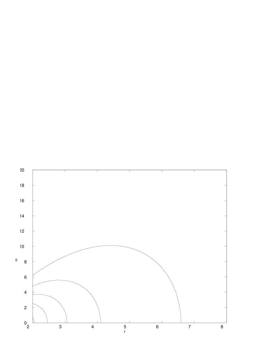
Figure 1: Disk structure for a typical case. Contours of the density (in units of $\tilde{\rho}$) are plotted in the $r-z$ plane. Note that due to the different scalings the figure actually presents a vertically stretched disk by a factor of $\epsilon^{-1}\sim 50$

Figure 2 is the vertical temperature profile $T(z)$ for a representative radius value and two values of $\alpha$: $0.4$ (the solid line) and $0.7$ (the dotted line). As we shall see in the next section, these two cases differ radically in their meridional flow pattern, but we should stress that the temperature profiles described here are calculated in the lowest order and are, of course, not influenced by the flow.

The procedure outlined in this section provides the lowest order values of the disk structure functions $p_{0}(r,z)$, $\rho_{0}(r,z)$ and so on, which will be needed to solve for the flow pattern in the next order.

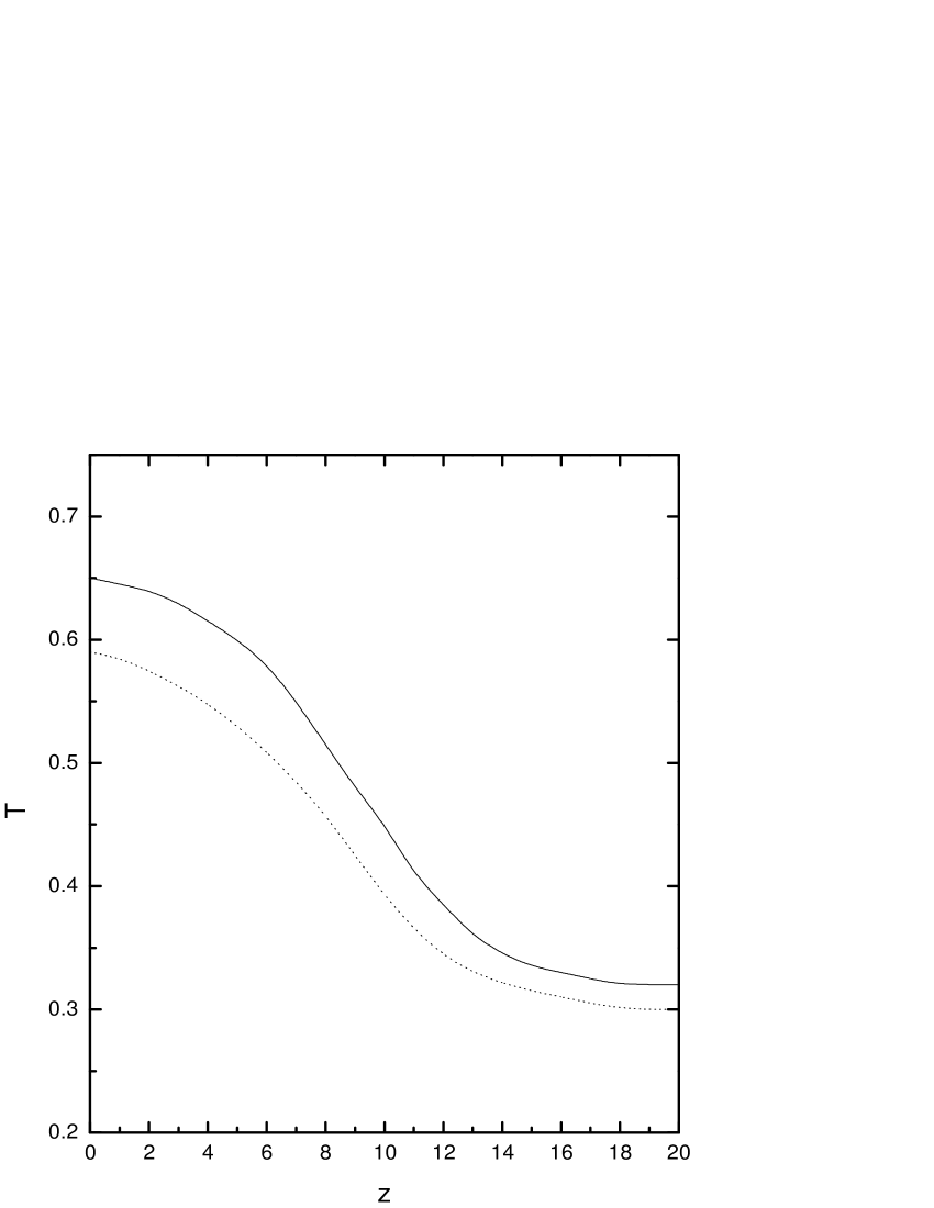
Figure 2: Vertical temperature profiles for a typical radius in the disk. The non-dimensional temperature is shown as a function of $z$ (in units of $\epsilon r_{+}$) for $\alpha=0.4$ (solid line) and $\alpha=0.7$ (dotted line)

4 Higher order solutions - the meridional flow pattern

As explained above, the lowest order contributions to the meridional velocity componenets are of order $\epsilon$ (i.e. $u_{1}$) and $\epsilon^{2}$ (i.e. $v_{2}$) and it turns out that the lowest order correction to the Keplerian angular velocity is of order $\epsilon^{2}$ ($\Omega_{2}$) - see KK and Urpin (urpin (1984)). The relevant equations, following from the expansions and originating from the mass, angular momentum and horizontal momentum conservation equations are

$$\partial_{r}(r\rho_{0}u_{1})+r\partial_{z}(\rho_{0}v_{2})=0,$$ (22)

$$r\rho_{0}u_{1}\partial_{r}(r^{2}\Omega_{0})=\partial_{r}(\eta r^{3}\partial_{r}\Omega_{0})+r^{3}\partial_{z}(\eta\partial_{z}\Omega_{2}),$$ (23)

$$-2r\rho_{0}\Omega_{0}\Omega_{2}={3z^{2}\over 2r^{4}}\rho_{0}-\partial_{r}p_{0}+\partial_{z}(\eta\partial_{z}u_{1}).$$ (24)

Despite their appearance these equations can be viewed as ODE in $z$ for any given $r$, since $p_{0}$, $\rho_{0}$ and $\Omega_{0}$, as well as $\eta$ are already known functions, from the lowest order solution for the vertical structure (as explained in the previous section). In addition, equation (22) can be decoupled from the other two, because one of the variables, $v_{2}$, appears only in it. Since equations (23-24) are of second order each, four boundary conditions are required. Two of them are obvious and are the result of equatorial symmetry:

$$\partial_{z}u_{1}=0\leavevmode\nobreak\ \leavevmode\nobreak\ \leavevmode\nobreak\ {\rm and}\leavevmode\nobreak\ \leavevmode\nobreak\ \leavevmode\nobreak\ \partial_{z}\Omega_{2}=0;\leavevmode\nobreak\ \leavevmode\nobreak\ \leavevmode\nobreak\ {\rm at}\leavevmode\nobreak\ \leavevmode\nobreak\ \leavevmode\nobreak\ z=0,$$ (25)

for any $r$. The other two conditions result from a regularity requirement, that is, that $u_{1}$ and $\Omega_{2}$ remain bounded for $z\to\infty$. In KK the density achieved a true zero for a finite value of $z$, owing this property to the polytropic assumption. In our case $\rho_{0}$ decays with $z$ and we have found that physically meaningful results are to be expected only if we require that both $\rho_{0}u_{1}$ and $\rho_{0}\Omega_{2}$ are sufficiently small at $z_{\rm out}$. This expectation has been strengthened by testing our algorithm on the polytropic case and getting very good agreement with the analytical results of KK.

After the two equations (23-24) are solved, $v_{2}$ follows from the solution of the first order equation (22) with the initial condition $v_{2}=0$ at $z=0$.

The result of a representative calculation ($\alpha=0.4$ and electron scattering opacity) is shown in Figure 3. For this case we obtain a meridional flow pattern with a backflow around the equatorial plane. The stagnation radius is in this case $r_{\rm stag}\sim 7.5r_{+}$.

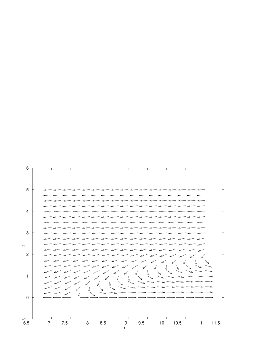
Figure 3: Meridional flow pattern with backflow. The flow is represented by the direction of streamlines at a grid of points in the $r-z$ plane. Note that the scale of $z$ is ”stretched” by a factor $\epsilon^{-1}\sim 50$

For other values of $\alpha$ the trend is similar to the one found by KK, that is, $r_{\rm stag}$ growing with $\alpha$ and for $\alpha>\alpha_{\rm crit}$ there are no solutions with backflows ($r_{\rm stag}=\infty$). While the disk structure depends somewhat on the opacity law (we have experimented with electron scattering opacity and Kramers opacity law), the meridional flow pattern and the stagnation radius (see below) are quite insensitive to it. In fact the relevant graphs (see below) for the abovementioned two opacity laws look indistinguishable and consequently we shall display only the electron scattering opacity case.

A case in which the stagnation radius is so large that it is not found up to $r\sim 1000r_{+}$ is shown in fig. 4, where $\alpha=0.7$. Note that even for these large values of $r$ the flow is directed inward everywhere.

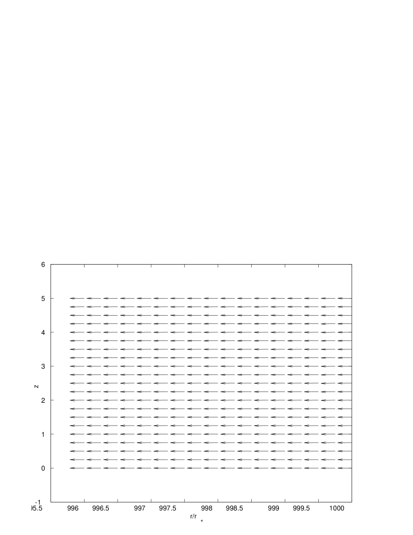
Figure 4: Meridional flow pattern with no backflow. The flow is represented by the direction of streamlines at a grid of points in the $r-z$ plane. Note that the scale of $z$ is ”stretched” by a factor $\epsilon^{-1}\sim 50$

The determination of the value of $\alpha_{\rm crit}$ can be achieved by calculating $r_{\rm stag}$ for a sequence of $\alpha$ values and finding where $r_{\rm stag}(\alpha)$ grows beyond any reasonable bound. Reasonable, in this context, means a radius beyond which the disk does not exist in a realistic astrophysical setting. In any case, when $r$ is very large the present numerical calculation cannot give reliable results because of the truncation error.

In Fig. 5 we show the stagnation radius for a number of $\alpha$ values and clearly see the trend that it grows beyond any reasonable bound for $\alpha\ga 0.7$. It is interesting to note that our results are completely consistent with the analytical result of KK (solid line) found for polytropes. The meridional flow behavior seems to result thus from the dynamics rather than from thermal processes in the disk.

5 Summary

In this work we have included thermal effects in the scheme, previously proposed by Kluźniak and Kita (1997), to calculate the vertical structure of thin accretion disks (including the flow pattern) by perturbative analysis. The small parameter of the expansions is $\epsilon$, reflecting the disk thickness. To the lowest order in $\epsilon$ the SS solution is recovered and we obtain also the vertical pressure and temperature structure. The accretion flow is found from the next order and includes, for small enough values of the viscosity parameter, equatorial backflows.

These findings support the claim made by KK that the backflows are of dynamical, rather than thermal, origin and probably result from vertical gradients of the viscous stress tensor. Our result for the flow is obtained numerically, using two explicit initial condition at the disk mid-plane and two regularity conditions. The latter complete the constraints needed for the solution of a fourth order differential system. However, because these constraints are independent of $r$, our solutions are obtained for all $r$ values and cannot account for given detailed boundary conditions on the flow at some $r=r_{out}$.

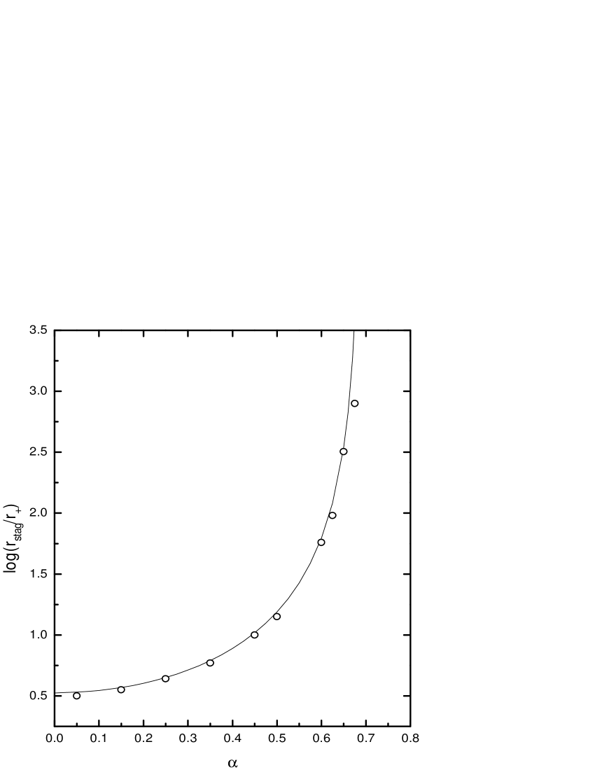
Figure 5: Logarithm of the stagnation radius (in units of $r_{+}$) as a function of $\alpha$. The circles are our numerical results while the solid line is the KK analytical solution for a polytrope.

Still, it is conceivable that if such conditions are imposed in a full numerical hydro simulation, our solution will be correct only for an intermediate region, situated between $r_{+}$ and $r_{\rm out}$, and not too close to these boundaries. Our solutions should smoothly join the outer flow pattern, which has to be consistent with the outer boundary conditions. For an outer boundary condition of inflow along all $z$, this should give rise to circulation patterns of the type observed in the numerical simulations of radiative disks cited in the introduction.

Although our results are formally valid only for very small $\epsilon$ and for radiative (as well as polytropic, see KK) disks, it is reasonable (as is often the case in asymptotic analyses of this type) that they carry over also to cases of $\epsilon$ close to unity. This means that quasi spherical flows, like the non-radiative ones (NRAF), may be endowed with circulation patterns as well. Whether these results are directly relevant to CDAF (if these flows are indeed proven to be viable) remains unclear. It can, however, be definitely stated that ADAF solutions using vertical averaging may not faithfully represent radial energy transport when there are substantial backflows, which naturally carry energy outwards in the hottest parts of the disk. In addition, we think that an approach of the kind reported here may provide useful tools for the understanding of some complicated features of flow patterns and instabilities in accretion disks.

References

- (1) Abramowicz, M.A., Chen, X.M., Kato, S., Lasota, J.-P., Regev, O., 1995, ApJ, 438, L37.
- (2) Abramowicz, M.A., Igumenshchev, I. V., 2001, ApJ, 554, L53.
- (3) Balbus, S.A., Hawley, J.F., 1991, ApJ, 376, 214
- (4) Balbus, S.A., Hawley, J.F., 1998, RevModPhys, 77, 204
- (5) Balbus, S.A., Papaloizou, J.C.B., 1999, ApJ, 521, 650
- (6) Bender, C.M., Orszag, S.A., 1999, Advanced Mathematical Methods for Scientists and Engineers, Springer
- (7) Frank, J., King, A.R., Raine, D.J., 2002, Accretion Power in Astrophysics, 3-rd ed., Cambridge.
- (8) Hawley, J.F., Balbus, S.A., Stone, J.M., 2001, ApJ, 554, L49.
- (9) Kley, W., Lin, D.N.C., 1992, ApJ, 397, 600.
- (10) Kluźniak, W., Kita, D., 1997, preprint: astro-ph0006266 (KK).
- (11) Lin, D.N.C., Papaloizou, J.C.B., 1996, ARA&A, 34, 703.
- (12) Narayan, R., Yi, I., 1994, ApJ, 428, L13.
- (13) Regev, O., 1983, A&A, 126, 146 (R83).
- (14) Różyczka, M., Bodenheimer, P., Bell, K.R., 1994, ApJ, 423, 736.
- (15) Shakura, N.I., Sunyaev, R.A., 1973, A&A, 24, 337 (SS).
- (16) Shaviv, G., Wickramasinghe, D., Wehrse, R., 1999, A&A, 344, 639.
- (17) Tassoul, J.-L., 1978, Theory of Rotating Stars, Princeton
- (18) Urpin, V.A., 1984, SvA, 28, 50.