Simultaneous Optical and X-ray Observations of Flares and Rotational Modulation on the RS CVn Binary
HR 1099 (V711 Tau) from the MUSICOS 1998 Campaign

We present simultaneous and continuous observations of the H$\alpha$, H$\beta$, He i D₃, Na i D₁,D₂ doublet and the Ca ii H & K lines for the RS CVn system HR 1099. The spectroscopic observations were obtained during the MUSICOS 1998 campaign involving several observatories and instruments, both echelle and long-slit spectrographs. During this campaign, HR 1099 was observed almost continuously for more than 8 orbits of $2\aas@@fstack{d}8$. Two large optical flares were observed, both showing an increase in the emission of H$\alpha$, Ca ii H & K, H$\beta$ and He i D₃ and a strong filling-in of the Na i D₁,D₂ doublet. Contemporary photometric observations were carried out with the robotic telescopes APT-80 of Catania and Phoenix-25 of Fairborn Observatories. Maps of the distribution of the spotted regions on the photosphere of the binary components were derived using the Maximum Entropy and Tikhonov photometric regularization criteria. Rotational modulation was observed in H$\alpha$ and He i D₃ in anti-correlation with the photometric light curves. Both flares occurred at the same binary phase (0.85), suggesting that these events took place in the same active region. Simultaneous X-ray observations, performed by ASM on board RXTE, show several flare-like events, some of which correlate well with the observed optical flares. Rotational modulation in the X-ray light curve has been detected with minimum flux when the less active G5 V star was in front. A possible periodicity in the X-ray flare-like events was also found.

1 Introduction

RS CVn binary systems consist of a chromospherically active evolved star tidally locked to a main-sequence or sub-giant companion. Short orbital periods of a few days are typically observed. The RS CVn high level of activity has been measured across the entire spectrum and, for fast rotators, it approaches the saturation limits for chromospheric, transition region and coronal emission. One of the striking aspects of these systems is their propensity to flare (Doyle et al. 1992). Moreover, RS CVns show optical photometric variations which are believed to arise from the rotational modulation of photospheric spots (Rodonò et al. 1986), large scale versions of dark solar spots, that provide evidence for large scale magnetic fields. The typical energies of the atmospheric magnetic fields in these systems are up to several orders of magnitude larger than on the Sun, thus allowing us to observe a range of energetic phenomena not occurring on the Sun. Short-period RS CVn-like systems, through their rotational modulation, can then provide information on the morphology and three-dimensional spatial distribution of spots in stellar atmospheres.

The system observed in this campaign is HR 1099 (V711 Tau, $03^{h}36^{m}47^{s}$ $+00^{o}35^{\prime}16^{\prime\prime}$ (J2000), V=5.64, B$-$V=0.92) a close double-lined spectroscopic binary. At a distance of 29 pc (The Hipparcos and Tycho Catalogues (ESA 1997)), HR 1099 is the nearest and brightest of the classical RS CVns with a K1 IV primary and a G5 V secondary tidally locked in a $2\aas@@fstack{d}8$ orbit. Fekel (1983) provided the orbital parameters of the binary and obtained masses, radii, and spectral types for both components. The K sub-giant nearly fills its Roche lobe and is by far the most “active” of the two components (Ayres & Linsky 1982; Robinson et al. 1996). Evolutionary models suggest that mass transfer from the K primary onto the G secondary may begin within $10^{7}$ years (Fekel 1983). The primary exhibits conspicuous signatures of chromospheric activity, such as strong and variable Ca ii H & K and H$\alpha$ emission (Rodonò et al. 1987; Dempsey et al. 1996; Robinson et al. 1996), which is due to its tidally induced rapid rotation, combined with the deepened convection zone of a post-main- sequence envelope. Montes et al. (1997) revealed broad and variable wings of the H$\alpha$ chromospheric line on the primary star.

Figure 1: The sites involved in the MUSICOS 98 campaign: INT, OHP, XING (Xinglong), KPNO (Kitt Peak), MSO (Mt. Stromlo), LNA, ESO and SAAO.

The G5 dwarf is probably also active, having a sufficiently deep convection zone and fast rotation to host an efficient dynamo. In particular, due to the presence of spots, G-type stars with rotation periods of about 3 days are expected to show V-band light curve amplitudes up to 0.10 mag, as can be inferred from the rotation-activity relations at photospheric levels (Messina et al. 2001). However, because of the small luminosity ratio in the V-band (L_G5V/L${}_{\rm K1IV}\simeq 0.27$), the contribution from the G5 component to the observed magnetic activity manifestations in the optical band is significantly smaller than from the K1 IV primary.

HR 1099 is one of the few RS CVn systems, along with UX Ari, II Peg, and DM UMa, that shows H$\alpha$ constantly in emission. Optical light curves have shown, via Doppler imagery, the presence of a long-lived ($>$11 yr) polar spot, together with transient ($<$1 yr) low-latitude spots on the surface of the active K star (Vogt et al. 1999). Strong magnetic fields of the order of 1000 G have also been detected on HR 1099 using the Zeeman Doppler Imaging technique (Donati et al. 1990, 1992; Donati 1999).

White et al. (1978) reported the first X-ray outburst in coincidence with a large radio flare on HR 1099. van den Oord & Barstow (1988) argued that the low amplitude variability of the HR 1099 light curve on time-scales of tens of minutes would indicate flare-like heating. This is in-keeping with the earlier work of Doyle & Butler (1985) who suggested that the corona of all late-type stars were heated via a flare-like process. Pasquini et al. (1989) suggested coronal temperatures of 3 MK and 25 MK based on spectral fits to the X-ray data. Several authors (Agrawal & Vaidya 1988; Drake et al. 1994; Audard et al. 2001) have reported periodic changes in the X-ray and UV light curves, which they attributed to rotational modulation of a starspot-associated bright coronal region. Dempsey et al. (1996) recorded, in coordinated IUE and GHRS observations, several flare enhancements in UV lines, one of which lasted more than a day. Wood et al. (1996) suggested a relationship between the broad wings in UV emission lines of HR 1099 and micro-flaring in its chromosphere and transition region. Brown et al. (1997) reported variability in high-energy bands with ASCA, RXTE, and EUVE: numerous small flares and a giant event lasting 3 days.

Table 1: The sites and instruments involved in the spectroscopic observation of HR 1099 during the MUSICOS 98 campaign and some of their most important characteristics: number of nights allocated at each site and instrument, resolving power, number of spectral orders, wavelength coverage (nm) and number of spectra obtained.

Site	Telescope	Spectrograph	Number	Resolving	Number	Wavelength	Number
			Nights	Power	Orders	coverage (nm)	Spectra
1. OHP, France	1.5 m	Aurelie	6	22 000	1	652-672	37
2. OHP, France	1.9 m	Elodie	8	43 000	67	390-690	7
3. KPNO, USA	0.9 m	Echelle	10	65 000	23	530-700	20
4. ESO, Chile	0.9 m	HEROS	11	20 000	62	350-560	34
					33	580-865	34
5. Mt.Stromlo, Australia	1.9 m	Echelle	5	35 000	43	480-680	17
6. Xinglong, China	2.2 m	Echelle	10	35 000	35	550-850	10
7. INT, Spain	2.5 m	ESA-MUSICOS	9	35 000	58	400-680	13
8. LNA, Brazil	1.6 m	Coudé	6	60 000	1	663-672	5
9. SAAO, South Africa	1.9 m	Giraffe	3	36 500	52	430-700	3

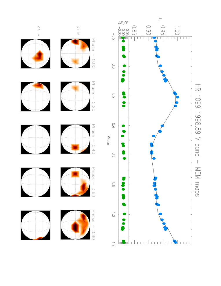
Figure 2: Top panel: V-band light curve (filled dots) of HR 1099 in late November/early December 1998 fitted by the Maximum Entropy spot model (continuous line). The flux was normalized to the brightest magnitude (V${}_{\rm unsp}=5.744$ at phase=0.21) and phases were computed according to Eq. (1). The residuals ($\Delta F/F$) between the observed and synthetized light curves are also plotted vs. phase. Bottom panel: Maps of the distribution along stellar longitude of the spot filling factors at five rotation phases. Spots located at latitude below $\simeq-33^{\circ}$ cannot contribute to the flux because the inclination of the star’s rotation axis is $33^{\circ}$.

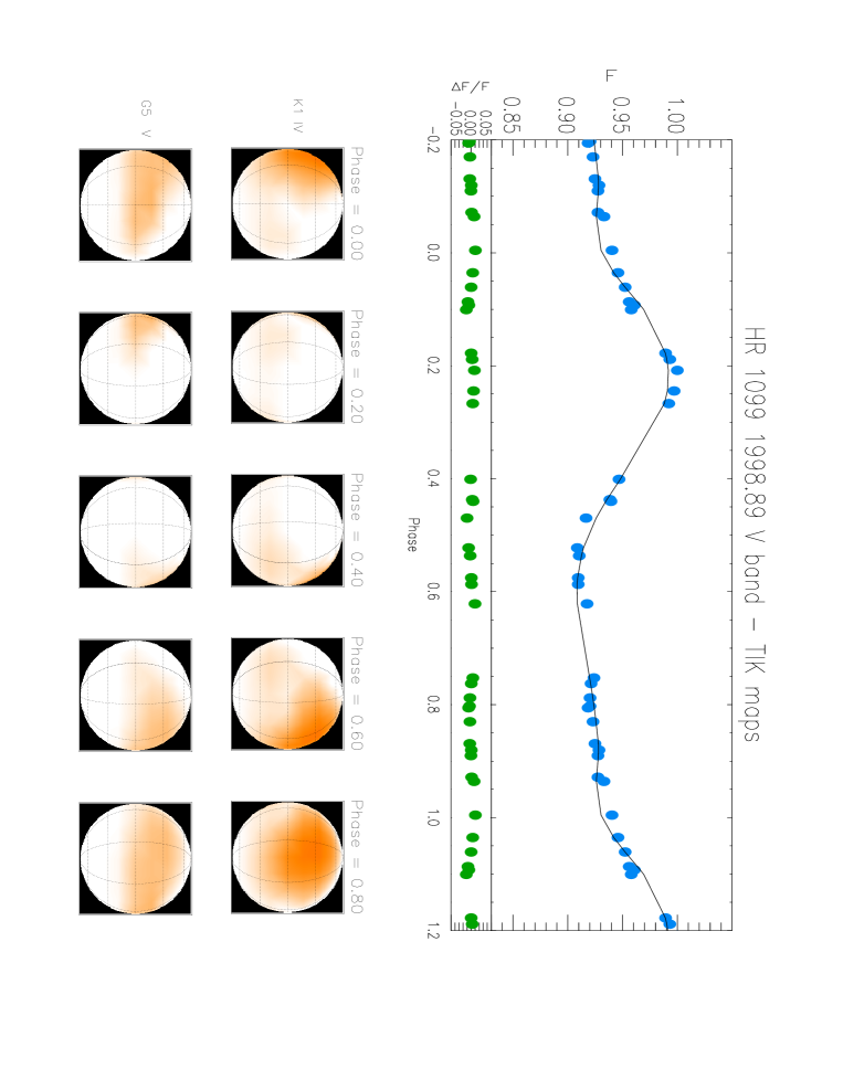
Figure 3: The same as in Fig. 2 fitted by the Tikhonov spot model and the Tikhonov photospheric maps. The presence of spots in the inaccessible regions is an artifact of the Tikhonov regularization that correlates the filling factors of nearby pixels.

Many scientific programs, most of them linked to stellar physics (such as flare monitoring, stellar rotational modulation, surface structures, Doppler imaging) requires continuous spectroscopic coverage over several days. MUSICOS (MUlti-SIte COntinuous Spectroscopy) is an international project for setting up a network of high resolution spectrographs coupled to telescopes well distributed around the world. During the MUSICOS 1989 campaign on HR 1099, Foing et al. (1994) obtained complete phase coverage for Doppler imaging of spots. They observed the modulation of the Ca ii K line profile due to chromospheric plage-like regions. They also observed two white-light flares (one of them was the largest optical flare reported on an RS CVn system) with typical rise and decay times of 60-90 min, and with a remarkable spectral dynamic signature in H$\alpha$. The fifth MUSICOS campaign (MUSICOS 98), the largest campaign organised to date, involved 13 telescopes to address 6 distinct science programs. Fig. 1 shows the distribution of the participating sites. The main goals of the campaign for HR 1099 were to monitor for flare events, to probe the chromospheric line variability in order to diagnose the energetics and dynamics in active regions, and to produce photospheric Doppler images.

In this paper we present the results of the MUSICOS 98 campaign on HR 1099. Observations and data analysis are described in Sect. 2; in Sect. 3 we present the results, and in Sect. 4 we analyse the flares on HR 1099. The conclusions are given in Sect. 5. Note that the fragmentary results from a preliminary analysis published in conference proceedings (García-Alvarez et al. 2002a, b) are superseded by the final ones presented herein.

Table 2: Log of the HR 1099 spectroscopic observations during the MUSICOS 98 campaign.

Date	JD	Phase	Exp.	Site	Date	JD	Phase	Exp.	Site
	2451100.0+		(sec.)			2451100.0+	mid exp	(sec.)
1998 Nov 21	39.390	0.6994	600	1	1998 Nov 30	48.046	0.7498	800	5
1998 Nov 21	39.430	0.7136	600	1	1998 Nov 30	48.147	0.7853	800	5
1998 Nov 21	39.494	0.7364	600	1	1998 Nov 30	48.333	0.8509	1200	1
1998 Nov 22	40.328	0.0300	1200	1	1998 Nov 30	48.356	0.8592	1200	1
1998 Nov 22	40.363	0.0425	1200	1	1998 Dec 01	48.519	0.9167	1800	4
1998 Nov 22	40.475	0.0819	1200	1	1998 Dec 01	48.597	0.9441	1800	4
1998 Nov 23	40.574	0.1169	1200	1	1998 Dec 01	48.932	0.0621	900	5
1998 Nov 23	40.659	0.1468	1200	1	1998 Dec 01	48.963	0.0731	800	5
1998 Nov 23	41.303	0.3739	600	2	1998 Dec 01	49.097	0.1203	800	5
1998 Nov 23	41.329	0.3829	1200	1	1998 Dec 01	49.144	0.1367	800	5
1998 Nov 23	41.367	0.3961	1200	1	1998 Dec 01	49.438	0.2402	600	1
1998 Nov 23	41.423	0.4160	600	2	1998 Dec 02	49.519	0.2691	1800	4
1998 Nov 23	41.470	0.4326	1200	1	1998 Dec 02	49.612	0.3017	1800	4
1998 Nov 24	41.569	0.4676	1200	1	1998 Dec 02	49.934	0.4152	900	5
1998 Nov 24	41.585	0.4732	1200	3	1998 Dec 02	50.011	0.4424	1200	6
1998 Nov 24	41.654	0.4975	1200	1	1998 Dec 02	50.074	0.4647	1200	6
1998 Nov 24	41.711	0.5175	900	3	1998 Dec 02	50.185	0.5036	1200	6
1998 Nov 24	41.853	0.5674	1200	3	1998 Dec 03	50.516	0.6203	1800	4
1998 Nov 24	41.959	0.6049	1200	3	1998 Dec 03	50.608	0.6528	1800	4
1998 Nov 24	42.319	0.7316	600	2	1998 Dec 03	50.975	0.7821	900	5
1998 Nov 24	42.327	0.7346	1200	1	1998 Dec 03	51.007	0.7933	800	5
1998 Nov 24	42.351	0.7429	1200	1	1998 Dec 03	51.066	0.8141	800	5
1998 Nov 24	42.451	0.7781	1200	1	1998 Dec 03	51.126	0.8354	800	5
1998 Nov 25	42.543	0.8107	1200	1	1998 Dec 03	51.184	0.8557	800	5
1998 Nov 25	42.584	0.8251	1200	3	1998 Dec 03	51.287	0.8922	1800	9
1998 Nov 25	42.627	0.8403	1200	1	1998 Dec 03	51.346	0.9127	1800	9
1998 Nov 25	42.735	0.8782	1200	3	1998 Dec 03	51.446	0.9480	900	9
1998 Nov 25	42.838	0.9145	1200	3	1998 Dec 04	51.514	0.9720	1800	4
1998 Nov 25	42.938	0.9499	1200	3	1998 Dec 04	51.610	0.0057	1800	4
1998 Nov 26	43.510	0.1516	1200	1	1998 Dec 04	52.035	0.1557	1200	6
1998 Nov 26	43.594	0.1812	1800	4	1998 Dec 04	52.062	0.1653	1200	6
1998 Nov 26	43.622	0.1907	1200	1	1998 Dec 04	52.168	0.2025	1200	6
1998 Nov 26	43.677	0.2103	1800	4	1998 Dec 04	52.247	0.2304	1200	6
1998 Nov 26	43.759	0.2392	1200	3	1998 Dec 05	52.513	0.3241	1800	4
1998 Nov 26	43.847	0.2700	1200	3	1998 Dec 05	52.598	0.3540	1200	7
1998 Nov 26	43.967	0.3124	1200	3	1998 Dec 05	52.606	0.3566	1800	4
1998 Nov 26	43.982	0.3177	1200	3	1998 Dec 05	53.088	0.5265	1200	6
1998 Nov 26	43.997	0.3231	1200	3	1998 Dec 06	53.514	0.6767	1800	4
1998 Nov 26	44.306	0.4318	1200	2	1998 Dec 06	53.614	0.7120	1800	4
1998 Nov 26	44.324	0.4384	1200	1	1998 Dec 06	54.479	0.0169	1200	7
1998 Nov 26	44.345	0.4457	1200	1	1998 Dec 07	54.511	0.0282	1800	4
1998 Nov 26	44.454	0.4842	1200	1	1998 Dec 07	54.606	0.0617	1800	4
1998 Nov 27	44.513	0.5050	1800	4	1998 Dec 07	54.669	0.0837	1500	7
1998 Nov 27	44.581	0.5289	1800	4	1998 Dec 07	55.108	0.2384	1200	6
1998 Nov 27	44.629	0.5458	1200	3	1998 Dec 07	55.170	0.2604	1200	6
1998 Nov 27	44.644	0.5510	1200	3	1998 Dec 07	55.347	0.3228	900	7
1998 Nov 27	44.659	0.5563	1200	3	1998 Dec 07	55.444	0.3571	600	8
1998 Nov 27	44.783	0.5999	1200	3	1998 Dec 07	55.469	0.3659	600	8
1998 Nov 27	44.798	0.6053	1200	3	1998 Dec 07	55.491	0.3735	1200	7
1998 Nov 27	44.812	0.6104	1200	3	1998 Dec 08	55.514	0.3815	1800	4
1998 Nov 27	44.941	0.6557	1200	3	1998 Dec 08	55.515	0.3820	600	8
1998 Nov 27	45.328	0.7923	1200	2	1998 Dec 08	55.612	0.4160	1800	4
1998 Nov 27	45.345	0.7981	1200	1	1998 Dec 08	56.330	0.6691	900	7
1998 Nov 27	45.462	0.8392	1200	1	1998 Dec 08	56.487	0.7246	1200	7
1998 Nov 28	45.513	0.8571	1800	4	1998 Dec 09	56.517	0.7349	1800	4
1998 Nov 28	45.549	0.8698	1200	1	1998 Dec 09	56.543	0.7442	600	8
1998 Nov 28	45.632	0.8992	1200	1	1998 Dec 09	56.550	0.7466	600	8
1998 Nov 28	46.324	0.1432	1500	2	1998 Dec 09	56.558	0.7493	600	8
1998 Nov 28	46.337	0.1476	1200	1	1998 Dec 09	56.613	0.7689	1800	4
1998 Nov 28	46.359	0.1554	1200	1	1998 Dec 09	57.364	0.0335	900	7
1998 Nov 28	46.454	0.1889	1200	1	1998 Dec 10	57.517	0.0873	1800	4
1998 Nov 29	46.523	0.2132	1800	4	1998 Dec 10	57.524	0.0897	900	7
1998 Nov 29	47.017	0.3872	900	5	1998 Dec 10	57.610	0.1203	1800	4
1998 Nov 29	47.031	0.3921	900	5	1998 Dec 10	58.302	0.3641	900	7
1998 Nov 29	47.156	0.4361	900	5	1998 Dec 10	58.341	0.3778	900	7
1998 Nov 29	47.374	0.5129	1500	2	1998 Dec 10	58.374	0.3893	1200	7
1998 Nov 29	47.397	0.5210	1200	1	1998 Dec 11	58.515	0.4389	1800	4
1998 Nov 30	47.513	0.5619	1800	4	1998 Dec 11	58.610	0.4727	1800	4
1998 Nov 30	47.542	0.5724	1200	1	1998 Dec 11	58.627	0.4786	900	7
1998 Nov 30	47.586	0.5878	1800	4	1998 Dec 12	59.511	0.7901	1800	4
1998 Nov 30	47.635	0.6052	1200	1	1998 Dec 12	59.612	0.8256	1800	4
1998 Nov 30	47.929	0.7087	900	5	1998 Dec 13	60.516	0.1442	1800	4
1998 Nov 30	47.967	0.7219	900	5	1998 Dec 13	60.644	0.1893	1800	4

Table 3: Log of RTXE observations.

Date	No. exp.	Exp. time
		(sec.)
1998 Nov 22	9	90
1998 Nov 23	13	90
1998 Nov 24	3	90
1998 Nov 25	12	90
1998 Nov 26	6	90
1998 Nov 27	16	90
1998 Nov 28	11	90
1998 Nov 29	17	90
1998 Nov 30	13	90
1998 Dec 01	7	90
1998 Dec 02	24	90
1998 Dec 03	33	90
1998 Dec 04	11	90
1998 Dec 05	11	90
1998 Dec 06	4	90
1998 Dec 07	22	90
1998 Dec 08	13	90
1998 Dec 09	11	90
1998 Dec 10	21	90
1998 Dec 11	11	90
1998 Dec 12	12	90

2 Observations and Data

2.1 MUSICOS 98 campaign: Optical Spectroscopy

The spectroscopic observations were obtained from 21 November to 13 December 1998 during the MUSICOS 98 campaign. It involved eight northern and southern sites, namely: Observatoire de Haute-Provence (OHP), Kitt Peak National Observatory (KPNO), European Southern Observatory (ESO), Mt. Stromlo Observatory (MSO), Xinglong National Observatory, Isaac Newton Telescope (INT), Laboratório Nacional de Astrofísica (LNA) and South African Astronomical Observatory (SAAO), using both echelle and long-slit spectrographs. A summary of the sites and instruments involved in the campaign and some of their most important characteristics are given in Table 1.

The spectra were extracted using the standard reduction procedures in the NOAO packages IRAF. For OHP, HEROS and Xinglong observations, the MIDAS package was used. Background subtraction and flat-field correction using exposures of a tungsten lamp were applied. The wavelength calibration was obtained by taking spectra of a Th–Ar lamp. A first-order spline cubic fit to some 45 lines achieved a nominal wavelength calibration accuracy which ranged from 0.06 to 0.11 Å. The spectra were normalized by a low-order polynomial fit to the observed continuum. Finally, for the spectra affected by water lines, a telluric correction was applied.

Apart from the chromospheric activity indicators, the spectra also include many lines important for spectral classification (i.e. Ca i triplet 6102, 6122, 6162 Å and Na i doublet 8183.3,8194.8 Å) and temperatures calibration purposes (i.e. V i 6251.8 Å and Fe i 6252.6 Å), as well as other lines normally used for the application of the Doppler imaging technique (i.e. Fe i 6411.7 Å, Fe i 6430.9 Å and Ca i 6439.1 Å). A summary of the observations, including Julian date, phase at mid-exposure and site (refer to Table 1), is given in Table 2. To produce a phase-folded light curve we adopted the ephemeris given in Eq. (1).

Appropriate data have been obtained to apply Doppler Imaging technique, based on the photospheric lines, to study the connection between spots, chromospheric emission and flares. These results will be presented in a separate paper (García-Alvarez et al. 2003).

2.2 RXTE X-ray Observations

The X-ray observations were obtained with the all-sky monitor (ASM) detector on board the Rossi X-ray Timing Explorer (RXTE) (Levine et al. 1996). The ASM consists of three similar scanning shadow cameras, sensitive to X-rays in an energy band of approximately 2-12 keV, which perform sets of 90-second pointed observations (“dwells”) so as to cover 80% of the sky every 90 minutes. The analysis presented here makes use of light curves obtained from individual dwell data. Light curves are available in four energy bands: A (1.3-3.0  keV), B (3.0-4.8  keV), C (4.8-12.2  keV) and S (1.3-12.2  keV). Around 15 individual ASM dwells of HR 1099 were observed daily by RXTE, during MUSICOS 98. A summary of the observations, including date, number of dwell data and exposure time are given in Table 3. The data were binned in four-hour intervals, which is approximately 6% of the orbital period of HR 1099.

2.3 Photometry

During the MUSICOS 98 campaign, ground-based photoelectric observations were obtained with two different Automatic Photoelectric Telescopes (APTs): a) the 0.80-m APT-80 of Catania Astrophysical Observatory (CAO) on Mt. Etna, Italy (Rodonò et al. 2001); b) the 0.25-m T1 Phoenix APT of Fairborn Observatory at Washington Camp, AZ, USA, that is managed as a multiuser telescope (Boyd et al. 1984; Seeds 1995). Both telescopes are equipped with standard Johnson UBV filters and uncooled photoelectric photometers. HR 1099 has been regularly monitored since 1988 by the Phoenix (Rodonò & Cutispoto 1992) and since 1992 also by the Catania APT-80 (Cutispoto et al. 1995). Although repeated observations were scheduled on each night during the campaign to obtain complete rotation phase coverage, bad weather conditions resulted in light curve gaps around phases 0.30 and 0.70.

Table 4: Radial velocities for the primary and secondary components of HR 1099, using the Fe i 6430.84 Å and Ca i 6439.07 Å lines, as measured from ESO-HEROS spectra.

JD	Orbital	$v_{r}$(km s-1) Fe i 6430.8 Å		$v_{r}$(km s-1) Ca i 6439.1 Å
2451100.0+	Phase	pri.	sec.	pri.	sec.
43.5940	0.1812	+34.16	$-78.32$	+32.03	$-77.83$
43.6770	0.2103	+33.50	$-76.18$	+32.55	$-77.47$
44.5810	0.5289	$-36.51$	+17.36	$-36.03$	+15.79
45.5130	0.8571	$-47.00$	+15.04	$-46.26$	+20.59
46.5230	0.2132	+33.18	$-76.55$	+32.19	$-77.47$
47.5130	0.5619	$-45.45$	+29.77	$-46.39$	+26.64
47.5860	0.5878	$-52.74$	+34.48	$-53.21$	+32.28
49.5190	0.2691	+28.56	$-72.72$	+27.53	$-72.90$
49.6120	0.3017	+25.99	$-66.80$	+24.16	$-65.76$
50.5160	0.6203	$-57.11$	+39.60	$-59.26$	+40.37
50.6080	0.6528	$-62.80$	+44.75	$-64.33$	+44.46
52.5130	0.3241	+22.42	$-61.27$	+19.45	$-61.26$
52.6060	0.3566	+17.32	$-50.55$	+11.32	$-51.53$
53.5140	0.6767	$-64.71$	+45.57	$-66.10$	+44.85
53.6140	0.7120	$-65.64$	+44.59	$-67.58$	+46.64
54.6060	0.0617	+19.05	$-55.85$	+14.34	$-56.33$
55.5140	0.3815	+08.37	$-41.22$	+04.84	$-41.94$
56.5170	0.7349	$-62.66$	+42.93	$-64.65$	+44.64
56.6130	0.7689	$-61.77$	+40.40	$-63.44$	+40.94
57.5170	0.0873	+23.24	$-63.28$	+20.73	$-64.19$
57.6100	0.1203	+27.11	$-71.24$	+25.62	$-71.17$
59.5110	0.7901	$-55.76$	+41.56	$-58.51$	+38.05
59.6120	0.8256	$-52.60$	+31.27	$-54.03$	+29.66
60.5160	0.1442	+32.30	$-73.47$	+28.96	$-74.52$
60.6440	0.1893	+32.98	$-78.28$	+31.57	$-78.86$

The Catania APT-80 observed HR 1099 differentially with respect to the comparison star HD 22796 (V=5.55, B$-$V=0.94) and the check star HD 22819 (V=6.10, B$-$V=1.00). The Phoenix APT observed HR 1099 differentially with respect to the comparison star HD 22484 (V=4.28, B$-$V=0.58), while HD 22796 (V=5.56, B$-$V=0.94) served as a check star. After subtraction of sky background and correction for atmospheric extinction, the instrumental differential magnitudes were converted into the standard Johnson UBV system. In order to obtain a homogeneous data set the measurements from the two telescopes were first converted into differential values with respect to the same comparison star HD 22796 and then converted into standard values. Details on the observation techniques, reduction procedures and accuracy of the Phoenix and the Catania APT-80 photometry are given in Rodonò & Cutispoto (1992) and Cutispoto et al. (2001), respectively.

The V-band flux modulation shown by HR 1099 in 1998.89 (see top panel of Fig. 2) can be attributed to the presence of a stationary spot pattern, mainly on the photosphere of the K1 IV primary, whose visibility is modulated by the stellar rotation. The HR 1099 light curve was computed using Fekel (1983) ephemeris:

$$HJD=2442766.080+2.83774E$$ (1)

All the APT observations included the faint visual tertiary companion HD 22468B (V_ter=8.83, Eggen (1966)), which is 6 arcsec away from the spectroscopic binary. Its contribution to the observed light curve is $\Delta V=-0.061$ mag. Before performing spot modelling, the V-band differential magnitudes were corrected for the third component’s contribution:

$$\Delta V$=$2.5\log(10^{-0.4\Delta V_{\mathrm{obs}}}-10^{-0.4(V_{\mathrm{ter}}-V_{\mathrm{comp}})})$$ (2)

From the light curve maximum V${}_{\rm max}=5.744$ at the 1998.89 epoch and assuming V $=$ 7.2 for the magnitude of the G5 component (Henry et al. 1995), the maximum of the primary K1 IV was estimated to be V $=$ 6.074.

3 Results

3.1 Radial Velocity and Orbital Solution

According to Fekel (1983), the orbital period has remained constant over 60 years. Therefore, to compute the observed phases for our analysis, we adopted his ephemeris (see Eq. (1)). The uncertainty in the period (0.00001 d) is small enough to ensure that, in the three week interval of our campaign, any possible phase drift is less than 0.001 cycles. We therefore solved for the following orbital parameters: $\phi_{0}$ (phase of conjunction with the K1 IV sub-giant in front), $\gamma$ (systemic velocity), $K_{pri},K_{sec}$ (semi-amplitudes of the velocity curves for the K1 IV and G5 V star, respectively). The radial velocities were determined by using a two-Gaussian fitting technique to each profile of Fe i 6430.84 Å and Ca i 6439.07 Å observed with HEROS on the Dutch 0.9 m telescope at ESO. This site was the only one that observed those photospheric lines during almost all the campaign. The individual profiles of each component were resolved and the velocity shifts were measured with respect to the laboratory wavelengths of the Fe i and Ca i lines. We obtained altogether 100 new velocities (25 for each component in the two photospheric lines) and used them to recompute the orbital parameters of HR 1099. These velocities are listed in Table 4. In order to obtain the orbital parameters, the radial velocity curves were fitted by a double-lined spectroscopic binary (SB2) model. Observations near phase conjunction between the components were not used because of line blending. The orbital parameters are listed in Table 5. Fig. 4 shows the observed and computed radial velocity curves for the two components of HR 1099, along with their (O-C) residuals.

Figure 4: Observed and computed radial velocity curves for the two components of HR 1099. Measurements for the K1 sub-giant and G5 are plotted as filled and open symbols, respectively. Velocities from Fe i 6430 Å and Ca i 6439 Å are denoted by coupled symbols. The dashed line is the system’s radial velocity. Plus and asterisk symbols show the radial velocities, calculated using H$\alpha$, during the optical flares at JD 2451145.51 and JD 2451151.07, respectively. The (O-C) velocity residuals are shown in the bottom panel.

Table 5: Orbital elements for the HR 1099 system.

Element (Unit)	Value
$P_{\mathrm{{orb}}}$ (days)	2.83774 (adopted)
T0(HJD)	2451142.943  $\pm$ 0.002
$\gamma$ (km s1)	$-15.61$ $\pm$ 0.20
$K_{\mathrm{{pri}}}$ (km s1)	49.66 $\pm$ 0.34
$K_{\mathrm{{sec}}}$ (km s1)	62.88 $\pm$ 0.70
$\phi_{0}$	$-0.0478$
$e$	0.0 (adopted)
$a_{1}$ sin $i$ (km)	1.94 $\pm$ 0.01 x 106
$a_{2}$ sin $i$ (km)	2.45 $\pm$ 0.03 x 106
$a$ sin $i$ (km)	4.39 $\pm$ 0.03 x 106
$M_{1}$ sin${}^{3}\,i$ (M☉)	0.234 $\pm$ 0.005
$M_{2}$ sin${}^{3}\,i$ (M☉)	0.185 $\pm$ 0.004
$M_{1}$/$M_{2}$	1.266 $\pm$ 0.011
RMS for solution (km s-1)	1.85

Table 6: A comparison of orbital parameters for HR 1099. $K_{\rm pri}$ and $K_{\rm sec}$ denote the velocity amplitudes of the primary and the secondary, respectively. $\gamma$ is the systemic velocity, and $\phi_{0}$ is the orbital phase of the superior conjunction (primary in front).

Reference	$K_{\mathrm{pri}}$	$K_{\mathrm{{sec}}}$	$\gamma$	$\phi_{0}$
		(km s-1)
This paper	49.7	62.9	$-15.6$	$-0.0478$
Strassmeier & Bartus (2000)	52.6	64.1	$-15.9$	$-0.0384$
Donati (1999)	50.0	63.1	$-14.3$	$-0.0378$
Donati et al. (1992)	50.0	62.8	$-15.4$	+0.008
Fekel (1983)	49.4	61.7	$-15.0$	0

In Table 6 we compare our derived orbital parameters with previous determinations. The results of our analysis are in good agreement with those obtained by previous authors. The value we found for $\phi_{0}$ seems to support previous results by Donati (1999) and Strassmeier & Bartus (2000), who suggested a slow but significant variation of the orbital phase at superior conjunction with time; providing evidence for orbital period variation. Applegate (1992), and most recently Lanza & Rodonò (1999), interpreted such a variation as a change of the quadrupole-moment of the primary, along the activity cycle, arising from cyclic exchanges between kinetic and magnetic energy driven by a hydromagnetic stellar dynamo. Such a mechanism has been used by Kalimeris et al. (1995) to explain the orbital period variations in another RS CVn system: SZ Psc. Fekel (1983) estimated an orbital inclination of $33^{o}\,\pm\,2^{o}$, this value also used by Vogt & Penrod (1983) and Vogt et al. (1999). Although Donati (1999) preferred a value of $40^{o}\,\pm\,5^{o}$, we keep the inclination fixed at $33^{o}$ for all further calculations. Adopting this inclination angle and the values of $K_{\rm pri}$ and $K_{\rm sec}$, the derived masses of the components of HR 1099 are: $M_{1}=1.45M_{\sun}$; $M_{2}=1.14M_{\sun}$.

3.2 Photometry and Spot Modelling

The properties of the photospheric spotted regions or, more precisely, of the total spotted area and its distribution versus stellar longitude, can be obtained by analysing the rotational modulation of the optical band flux. However, due to the low information content of wide-band photometry, the derived maps are not unique. In order to obtain unique and stable solutions, some a priori constraints on the properties of the photospheric maps, that is a regularization criterion, must be assumed. In the present study we used both the Maximum Entropy method (hereafter ME, Vogt et al. 1987) and the Tikhonov criterion (hereafter T, Piskunov et al. 1990).

The star’s surface is divided into pixels and the specific intensity of the $i$-th pixel is assumed to be given by

$$I_{i}=f_{i}I_{s}+(1-f_{i})I_{u}$$ (3)

where I_u and I_s = C_s I_u are the specific intensity of the unspotted and spotted photosphere of the $i$-th pixel (C_s is the brightness contrast which we assume to be constant) and $0\leq f_{i}\leq 1$ is the pixel fraction covered by spots. The final map is obtained by finding the distribution of $f_{i}$ that gives a constrained extreme of the ME or T functionals, subject to a $\chi^{2}$ limit. A detailed description of our modelling approach, source of errors and accuracy can be found in Lanza et al. (1998).

The numerical code we used to compute the solutions adopts Roche geometry to describe the surfaces of the components and Kurucz’s atmospheric models to compute the surface fluxes and linear limb-darkening in the V-band (Lanza et al. 2001). Gravity darkening and reflection effect coefficients were introduced according to the procedure outlined by Lanza et al. (1998). The stellar and model parameters adopted to compute the final maps are listed in Table 7.

Table 7: Stellar and model parameters of HR 1099 assumed to compute the photospheric maps.

Stellar parameters	K1 IV	G5 V	Ref.
Brightest V magnitude	6.074	7.2	1
V-band fractional luminosity	0.784	0.215	2
Limb-darkening coeff. (unspotted)	0.792	0.734	3
Limb-darkening coeff. (spotted)	0.823	0.798	3
Cs	0.161	0.318	3
Bolometric correction (mag)	-0.50	-0.10	3
Gravity darkening	0.25	0.25	4
Surface gravity log $g$ (cm sec-2)	3.30	4.26	5
Effective temperature (K)	4750	5500	6
Starspot temperature (K)	3750	4500	7
Roche potential	3.8624	19.6412	4
Fract. radius (point)	0.3572	0.1070	4
Fract. radius (side)	0.3330	0.1067	4
Fract. radius (pole)	0.3225	0.1066	4
Fract. radius (back)	0.3465	0.1070	4

[1] see Sect. 2.1; [2] present paper; [3] Kurucz’s models (2000);
[4] Kopal (1989); [5] according to mass and radius;
[6] Donati (1999); [7] Strassmeier & Bartus (2000).

As shown in Figs. 2 & 3, a single large spotted region is present on the K1 IV primary, centered around phase 0.85. A much smaller spotted region in the ME map, about 45 degrees apart from the primary, is not resolved in the T solution, which represents the smoothest map that fits the light curve. Spots are also present on the secondary G5 component, centered around phase 0.0 and their area is smaller than on the K1 IV component.

The resulting spot pattern appears to be concentrated on the northern hemispheres of both components. This is due to the fact that spots located at latitudes below $\simeq-33^{\circ}$ cannot contribute to the variation of the observed flux because of the low value ($i\simeq 33^{\circ}$) of the inclination of the rotation axis. The ME modelling tends to minimize the total spotted area (A${}_{\rm ME}=5.49\%$ for K1 IV, A${}_{\rm ME}=1.60\%$ for G5 V), giving more compact and darker surface inhomogeneities. The T modelling tends to smooth the intensity fluctuations correlating the filling factors of nearby pixels and leads to photospheric maps with huge and smooth spots (A${}_{\rm T}=5.65\%$ for K1 IV, A${}_{\rm T}=3.14\%$ for G5 V). Lanza et al. (1998) pointed out that the regularized maps should be regarded as an intermediate step of the analysis. They must be used to derive quantities not depending on the regularizing criterion adopted, that is the distribution of the spots vs. longitude and its variation in time. Actually, apart from the different total spotted area between the ME and T solutions, both regularizing criteria reproduce a similar distribution of spotted area versus stellar longitude.

Absolute properties of the spots cannot be extracted from single-band data because systematic errors arise from the unknown unspotted light level, which we had to assume to coincide with the brightest magnitude at the 1998.89 epoch, and the assumption of single-temperature spots.

It is interesting to point out that both optical flares detected during the MUSICOS 98 campaign at JD 2451145.51 and JD 2451151.07, started around phase=0.80, that is at the rotation phase where the largest active region on the K1 IV component was facing the observer. Unfortunately, no simultaneous photometric observations were obtained at those epochs because of bad weather conditions.

3.3 Chromospheric Activity Indicators

The spectra presented in this paper allow us to study the behaviour of the different optical chromospheric activity indicators such as: Na i D₁, D₂ doublet, (formed in the upper photosphere), Ca ii H & K lines (lower chromosphere), H$\alpha$, H$\beta$ (middle chromosphere), and He i D₃ (upper chromosphere), as well as a large number of photospheric lines which can in some instances be affected by chromospheric activity (i.e. Fe i 3906.5 Å, Mn i 5341.1 Å, Fe i 5430.0 Å .. see Doyle et al. (2001)).

In Figs. 5-8 we show the time series of the Ca ii H & K lines, H$\alpha$, H$\beta$, Na i D₁, D₂ doublet and He i D₃ observed during the MUSICOS 98 campaign. The vertical axis represents the accumulative orbital phase, the first orbital revolution beginning at zero orbital phase.

We have measured the equivalent width (EW) for six lines with respect to a local continuum interpolated by a linear fit to line-free nearby continuum portions included within the covered spectral interval. The wavelength intervals are 6557.5–6566.5 Å for H$\alpha$, 5883.0–5903.0 Å for Na i D₁, D₂ doublet, 5872.0–5877.5 Å for He i D₃, 4857.5–4865.5 Å for H$\beta$, 3964.5–3972.5 Å for Ca ii H and 3929.7–3937.7 Å for Ca ii K. In this analysis we consider positive and negative values of the EW as referring to lines in absorption and emission, respectively. In Fig. 9 we plot the equivalent width measured for the H$\alpha$, Na i D₁, D₂ doublet, He i D₃, H$\beta$ , Ca ii H and Ca ii K lines, versus Julian date and the orbital phase.

Figure 5: Time series of the H$\alpha$ line, obtained during the entire 3-week MUSICOS 98 campaign. The vertical scale indicates the accumulative orbital phase. The vertical lines correspond to the rest wavelength of the line (solid line) and the corresponding maximum rotational broadening of the K1 IV component of $v\,\sin\,i=\pm\,41\ \mathrm{km\,s^{-1}}$ (dotted line), respectively.

Figure 6: Same as Fig. 5, but for the He i D₃ and Na i D₁, D₂ doublet.

Figure 7: Same as Fig. 5, but for the H$\beta$ 4861 Å line.

Figure 8: Same as Fig. 5, but for the Ca ii H & K lines. Note that the gap between spectra has been doubled for clarity sake.

3.4 Rotational Modulation

We have observed an increase in emission in the EW of the He i D₃ line and the Na i D₁, D₂ doublet, between $\phi=$0.5 and $\phi=$1.0 (see the second and third right panel of Fig. 9). These changes in EW are consistent with rotational modulations in the He i D₃ line, that could be attributed to pumping of the chromospheric emission by coronal X-rays from an overlying active region. A similar behaviour can be seen in the EW of the H$\alpha$ line with an increase in emission between $\phi=$0.7 and $\phi=$1.0 (see the top right panel of Fig. 9). These enhancements are unlikely to be a temporary, flare-like phenomenon, since they have been observed for almost nine rotations of the star. Note that the flares observed during the campaign correspond to significantly larger increases in emission in the EW (see Fig. 9). The H$\beta$ and the Ca ii H & K lines do not show any obvious rotational modulation. Such rotational modulation behaviour in chromospheric lines has been observed previously in other RS CVn systems (Rodonò et al. 1987; Busà et al. 1999; Padmakar et al. 2000). It may indicate that the distribution of chromospheric active regions is ascribed to localised regions and not uniformly distributed over the stellar surface, which would not produce any rotational signature. This vertical structure would resembles that of solar active regions.

The observed behaviour in the Na i D₁, D₂ doublet, the He i D₃ and H$\alpha$ lines, seems to show a sort of anti-correlation with the optical light curve (cf. Figs. 2 & 3). It means that the chromospheric emission maximum is in close coincidence with the minimum of the light curve (when the largest spotted region is facing the observer).

4 Flares Analysis

During the campaign, two optical flares were observed, one at JD 2451145.51 (28-11-98) lasting about 0.63 days and a second flare at JD 2451151.07 (03-12-98) lasting about 1.1 days (see Fig. 9).

4.1 The Hydrogen Balmer lines

4.1.1 The H$\alpha$ and H$\beta$ lines

The emission or filling-in of the H$\alpha$ (6562.8 Å) and H$\beta$ (4861.3 Å) lines is one of the primary optical indicators of chromospheric activity in RS CVn systems.

The first optical flare, at JD 2451145.51, shows an increase in emission in the measured EW by almost a factor of two in H$\alpha$. Broad components are observed at the beginning and at the maximum of this flare (see left panel of Fig. 10). The H$\alpha$ profile at the start of the flare has a full-width half maximum (FWHM) of 2.87 Å (equivalent to 131 $\mathrm{km\,s^{-1}}$) and shows a noticeable blue wing excess in four flare spectra. The largest FWHM, with a value of 4.52 Å (207 $\mathrm{km\,s^{-1}}$), was obtained for the spectrum at $\phi$=0.7981. The spectrum at $\phi$=0.8571, which corresponds to the maximum H$\alpha$ emission, has a FWHM of 3.47 Å (159 $\mathrm{km\,s^{-1}}$). A narrow absorption feature was also observed in this spectrum (see Fig. 10). Observations of the H$\beta$ line were not made during most of the flare, however, the spectrum observed around flare maximum, at $\phi$=0.8571, did show a filling-in of the H$\beta$ line (see Fig. 9 and top right panel in Fig. 10).

The second optical flare, at JD 2451151.07, shows an increase in emission in the measured EW by a factor of four in H$\alpha$. The left panel in Fig. 11 shows very broad components at the beginning and at the maximum of this event. The H$\alpha$ profile at the start of the second flare, $\phi$=0.6203, has a FWHM of 3.13 Å (equivalent to 141 $\mathrm{km\,s^{-1}}$). The largest FWHM, with a value of 3.82 Å (175 $\mathrm{km\,s^{-1}}$), was obtained for the spectrum at $\phi$=0.8141. The spectrum at $\phi$=0.8354, which corresponds to the maximum H$\alpha$ emission, has a FWHM of 3.71 Å (170 $\mathrm{km\,s^{-1}}$). The spectra before and after flare maximum show a symmetrical broadening, with a base width for the blue and red wings, of 6.25 Å (286 $\mathrm{km\,s^{-1}}$). Similar values for the FWHM were found by Foing et al. (1994) for another flare in the HR 1099 system. During this second optical flare, the H$\beta$ line turns into emission (see right panel of Fig. 11). We measured a FWHM of 2.33 Å (144 $\mathrm{km\,s^{-1}}$) for the spectrum at $\phi$=0.8144. It is slightly larger than the FWHM obtained during the flare maximum at $\phi$=0.8354, which was 2.14 Å (132 $\mathrm{km\,s^{-1}}$). The absorption feature in the H$\beta$ emission spectra around flare maximum may be due to the secondary star.

Figure 9: The equivalent width as a function of Julian date and as a function of phase for H$\alpha$, Na i D₁,D₂ doublet, He i D₃, H$\beta$ and Ca ii H & K lines observed at the different sites, namely: OHP152 (open circle), OHP193 (+), KPNO (open diamond), ESO (filled diamond), Mt.Stromlo (open triangle), Xinglong (*), INT (open square), LNA (filled square) and SAAO (filled triangle).

Apart from the two optical flares, H$\alpha$ showed flux enhancements around JD 2451143.0, 2451156.5 and 2451157.3. These JDs correspond to phases between 0.8 and 0.9. Also two enhancements were observed in the H$\beta$ line at around JD 2451155.0 and 2451157.3. Hereafter, we will refer as flare-like to those events which show an enhancement in the average line emission although, they may not be proper flares.

4.1.2 The Balmer Decrement

Balmer decrements (flux ratio of higher series members to H$\gamma$) have been used to derive plasma densities and temperatures in flare star chromospheres (Kunkel 1970; Gershberg 1974; Katsova 1990; García-Alvarez et al. 2002). Lacking H$\gamma$ data in our spectra, we have instead calculated the Balmer decrement from the $\rm{EW_{\mathrm{H\alpha}}/EW_{\mathrm{H\beta}}}$ ratio. During quiescent phases we obtained values around 1 for the $\rm{EW_{\mathrm{H\alpha}}/EW_{\mathrm{H\beta}}}$ ratio, while during the first flare we obtained slightly larger values (2-3). During the second flare the ratio even reached values of 8. This behaviour shows (unsurprisingly) a significant change in the properties of hydrogen emitting regions during the flare. Kunkel (1970) showed that this behaviour is possible if the Balmer lines are driven toward local thermodynamic equilibrium (LTE) conditions within an emitting region with an electron density of $n_{\rm e}\sim$10¹³ cm^-3, an electron temperature of $T_{\rm e}\sim$2$\times 10^{4}$ K, and a micro-turbulence velocity $\xi\sim$20 $\mathrm{km\,s^{-1}}$.

Figure 10: The observed spectra for H$\alpha$ (left panel), He i D₃, and Na i D₁,D₂ doublet (middle panel), H$\beta$ (upper right panel) and Ca ii H & K (lower right panel) of the first monitored flare starting at JD 2451145.51, arranged in order of the orbital phase. The vertical lines correspond to the rest wavelength of the lines (solid line) and the corresponding maximum rotational broadening of the K1 IV component of $v\,\sin\,i=\pm\,41\ \mathrm{km\,s^{-1}}$ (dotted line), respectively.

4.2 The Na i D₁, D₂ doublet

The Na i D₁ 5895.92 Å and D₂ 5889.95 Å lines are well known temperature and luminosity indicators. These resonance lines are collisionally-controlled in the atmospheres of late-type stars, providing information about chromospheric activity (Montes et al. 1997) and for M dwarfs they have been used to construct model atmospheres (Andretta et al. 1997). Unfortunately, the observations of the Na i D₁, D₂ doublet were not made during most of the first optical flare. However, the spectra observed around flare maximum, at $\phi$=0.8571, did show a slight filling-in (see Fig. 9 and the top middle panel of Fig. 10). During the second optical flare, the Na i D₁, D₂ doublet showed a strong filling-in, which during the maximum of this event, turned into emission reversal (see the middle panel of Fig. 11). Another flare-like event seems to have happened at around JD 2451155.0.

4.3 The He i D₃ line

Perhaps the most significant observation in support of flare-like events is the detection of emission in the He i D₃ line at 5876 Å. This line has a very high excitation level. It has been previously detected in absorption in active stars and attributed to plages or coronal radiation (Huenemoerder 1986). It has also been seen in emission during stellar flares (Montes et al. 1997, 1999; Oliveira & Foing 1999). In the Sun, it is in emission in the strongest flares (Tandberg-Hanssen 1967). As for Na i, observations of He i D₃ were not made during most of the first optical flare. However, the only spectrum observed around flare maximum, at $\phi$=0.8571, did not show any apparent change (see the top middle panel in Fig. 10). During the second optical flare, the He i D₃ line turns into emission (see the middle panel of Fig. 11). We measured a maximum FWHM of 0.88 Å (45 $\mathrm{km\,s^{-1}}$) for the spectra at $\phi$=0.7983. During flare maximum, $\phi$=0.8354, we measured a FWHM of 0.83 Å (42 $\mathrm{km\,s^{-1}}$). Fig. 9 shows that, during the second optical flare, the He i D₃ line peaks before the Balmer lines, in agreement with the emission line behaviour observed in late-type star flares (Garcia Alvarez 2000; Oliveira & Foing 1999). Three flare-like events seem to happen at around JD 2451148.0, 2451156.5 and 2451159.6. These JDs correspond to phases between 0.8 and 0.9.

4.4 The Ca ii H & K lines

The Ca ii H & K resonance lines have long been the traditional diagnostic of chromospheric activity in cool stars since they were studied by Wilson (1978). Observations of the Ca ii H & K lines were not made during most of the first optical flare. However, the spectra observed around the maximum during both flares, did show a small increase in flux (see the bottom panels of Fig. 9 and Fig. 10). Note that the Ca ii H & K lines peaked later than the Balmer lines, at around $\phi$=0.95. This behaviour has been observed in flares on late-type stars (Rodonò et al. 1988; Garcia Alvarez 2000).

Figure 11: The observed spectra for H$\alpha$ (left panel), He i D₃ and Na i D₁,D₂ doublet (middle panel) and H$\beta$ (right panel) of the second monitored flare starting at JD 2451151.07 arranged in order of the orbital phase. The vertical lines correspond to the rest wavelength of the lines (solid line) and the corresponding maximum rotational broadening of the K1 IV component of $v\,\sin\,i=\pm\,41\ \mathrm{km\,s^{-1}}$ (dotted line), respectively.

4.5 Flare Location

In Fig. 4, together with the radial velocity calculated using the photospheric lines, we have plotted the radial velocity for the two monitored flares. These radial velocities have been calculated by fitting a single Gaussian to the H$\alpha$ profile. The velocity shifts were measured with respect to the rest wavelength of the H$\alpha$ line. Despite the broad component developed by the H$\alpha$ line during flares, this seems to be a reliable fit. As a result, we notice that during both flares, the radial velocity is slightly displaced (15-20 $\mathrm{km\ s^{-1}}$) compared to the center of gravity of the primary. This could arise if both flares took place off the disk of the primary star.

Note that both flares took place at around the same phase (0.85), but $\sim$6 days apart suggesting a link between them and the active region complex, which was crossing the central meridian around that phase. The largest photospheric active region on the K1 IV component was indeed centered around $\phi$=0.85 (see Fig. 2 and Fig. 3). This behaviour is consistent with the proposed link between flares and surface active regions. During the MUSICOS 89 campaign, Foing et al. (1994) reported on a flare that took place again at a similar phase (0.87), suggesting that, if this is indeed the same active region, it is a long-lived feature. Vogt et al. (1999) analysed Doppler Images of HR 1099 and also proposed similar long-lived active regions.

Table 8: The energy released per exposure (in units of $10^{33}$ ergs) by the chromospheric lines during the optical flares observed on HR 1099 in the MUSICOS 98 campaign.

JD	phase	H$\alpha$	Na i D1,D2	He i D3	H$\beta$
2451100.0+
FLARE 1
45.328	0.7923	0.92	–	0.22	2.19
45.345	0.7981	0.50	–	–	–
45.462	0.8392	1.42	–	–	–
45.513	0.8571	2.90	0.06	0.17	1.60
45.549	0.8698	1.52	–	–	–
45.632	0.8992	1.25	–	–	–
FLARE 2
50.975	0.7821	0.62	0.14	0.03	1.21
51.007	0.7933	3.32	3.50	0.28	3.85
51.066	0.8141	5.29	3.49	0.85	5.59
51.126	0.8354	6.09	2.44	0.56	5.43
51.184	0.8557	5.51	1.46	0.35	4.98

4.6 Energy released

In order to estimate the energy released in the observed optical chromospheric lines during both optical flares, we converted the excess EW (flare EW minus quiet EW of the studied lines) into absolute surface fluxes and luminosities. Since we have not observed the entire flare, and several important lines are missing (e.g., Ly$\alpha$, Mg ii h&k, He i 10830 Å), our estimates are only lower limits to the total flare energy in the chromospheric lines. We have used the calibration of Hall (1996) to obtain the stellar continuum flux in the H$\alpha$ region as a function of ($B-V$) and then converted the EW into absolute surface flux. For the other lines, we have used the continuum flux at H$\alpha$ corrected for the continuum flux ratio $F_{\lambda 6563}/F_{\lambda}$. This $F_{\lambda}$ is given by a blackbody, with contribution of both the cool and the hot component of HR 1099 at $T_{\mathrm{eff}}=4\,840\ \mathrm{K}$ and $T_{\mathrm{eff}}=5\,460\ \mathrm{K}$, respectively. The contribution factors for each component has been obtained following the method by Montes et al. (1995). We converted these fluxes into luminosities using the radius $R=3.9\,R_{\sun}$, since we have assumed that both optical flares took place on the K1 IV component. Table 8 shows the energy released by the chromospheric optical lines for both flares. We obtained the flare energies by integrating the measured fluxes in time. Adding the energies for all the observed chromospheric lines during each flare, we obtained a total flare energy of $1.3\ 10^{34}$ erg for the first flare and $5.5\ 10^{34}$ erg for the second flare, integrating over a period of $\sim$7.3 and $\sim$5.5 hours respectively. These values for the energy released are comparable to other RS CVn flares (Doyle et al. 1991; Foing et al. 1994).

5 X-ray data

X-ray observations of HR 1099, with ASM on board RXTE, were carried out at the same time as the MUSICOS 98 campaign took place. In Fig. 12 we show the X-ray light curve of HR 1099 obtained by RXTE in the S band.

Figure 12: X-ray light curve observations of HR 1099, from the ASM instrument on RXTE satellite, obtained at the same time as the MUSICOS 98 campaign. The band S (1.5-12 keV) as a function of Julian date is shown. The spectroscopic optical observations during MUSICOS 98 campaign are shown on top of the X-ray data.

5.1 Long- and Short-Term Variability

The long-term light curve displays evident variability on short and long time-scales. We can divide the RXTE observations into three intervals, according to the observed activity levels. The X-ray data show a medium variability level between JD 2451139 and JD 2451145. In this first interval, which covered around two rotations, we see three possible flare-like events. A interval of low variability follows, covering approximately 1.5 rotations, between JD 2451145 and JD 2451149. Finally, the third interval, between JD 2451149 and JD 2451160, covering four rotations, exhibits strong variability. During this third term six possible X-ray flare-like events were observed. The flare-like events observed in the first and third intervals were only detected in the S and A bands but not in the B and the C bands. This suggests that these X-ray events were soft.

5.2 X-ray and Optical Flare Correlation

We have found that most of the optical flares show a X-ray counterpart. During the X-ray event at JD 2451143.02, a small increase in the emission of the H$\alpha$ was seen (see the top left panel of Fig. 9), as well as a filling-in in the Na i D₁, D₂ doublet. The optical flare observed at JD 2451151.07 was also observed in the X-ray range. The X-ray flare observed at JD 2451155.24 shows an optical counterpart in H$\beta$ line (see Fig. 9) and filling-in of the Na i D₁, D₂ doublet, although no clear variation was seen in either H$\alpha$ or He i D₃.

The flare-like event at JD 2451156.74 shows a small increase in the emission of H$\alpha$ and a small filling-in of the He i D₃ line (see Fig. 9). This enhancement was also observed in Ca ii H (not in K) suggesting that it reflects variability from H$\epsilon$. The possible flare observed at JD 2451157.24 shows a small increase in the H$\alpha$ and Ca ii H & K lines with also a small filling-in of the H$\beta$ line, but no changes are observed in the other lines. Conversely, the optical flare at JD 2451145.51 was not observed in any of the X-ray bands.

5.3 Flare Periodicity

We noted that most of the X-ray flares and flare-like events observed, took place either at $\phi\sim$0.31 (2451149.63 d, 2451152.54 d, and 2451155.24 d) or at $\phi\sim$0.91 (2451143.02 d, 2451151.23 d, 2451157.24 d and 2451159.64 d). Based on this fact one could say that there were two active regions, which flared during the same epoch. The flares of each active region show a rotation periodicity which lasted for almost three consecutive orbits, from JD 2451149 to JD 2451158, during what we have called the strong variability interval.

The possibility of rather persistent active longitudes in the photosphere is well known in the solar case. Leto et al. (1997) found evidence of a frequently flaring and persistent active longitude on EV Lac. This, coupled with rotation, may give rise to spurious periodicities or abnormally long-lasting flare events. Note that the X-ray flare-like event which would have been expected at JD 2451154.2, coupling with the one at JD 2451152.54, is not covered by X-ray observations. However, increases in the H$\beta$ and Ca ii H & K lines were observed at that epoch.

The observed rotational periodicity could have been caused by two very large flares, one on each active region, lasting for three consecutive orbits, which means that we have observed flares which lasted more than eight days!. This kind of long duration flares on active RS CVn stars has been previously observed by Montes & Ramsey (1998). However, one would expect an a exponential decay in the X-ray flux, which was not observed, and a much larger X-ray flux maximum, which was not observed either. So we discard a possible very long duration flare as an explanation for the observe X-ray light curve. Another possibility is suggested by the behaviour of the light curve at JD 2451150, JD 2451153 and JD 2451156. The X-ray flux appears to peak at $\phi\approx$0.31, after which it diminishes until it reaches a minimum when the G5 V star is in front of the active K1 IV star ($\phi$=0.5), in agreement with other authors (Drake et al. 1994; Audard et al. 2001; Sanz-Forcada et al. 2002). Similarly, Foing et al. (1994), observed a sudden flux decrease in an optical flare, that they suggest was caused by the occultation of the flaring active region, due to the rotation of the system. However, as a consequence of X-rays being optically thin, the rotational modulation they might produce would modulate the flare in an on-off fashion, but would not produce spiky flares as we observe in the X-ray light curve. Another possibility, is that we are looking at periodic flaring. Several authors have searched for such periodicity with mixed results (e.g. Lukatskaya 1976; Pettersen 1983; Doyle et al. 1990; Mullan & Johnson 1995; Mavridis et al. 1995). The confirmation of such a periodicity would support the idea of a “flare reservoir”, in other words, an active region with a certain amount of stored energy which is then released either as a single flare or as multiple of smaller events. Mullan & Johnson (1995) reported X-ray periodicities in late-type flare stars. They found that the observations were consistent with the hypothesis that resonant absorption of MHD waves were occurring at certain times in coronal loops. However, the preferred frequency inferred by Mullan & Johnson (1995) are much lower than the one we observed in HR 1099. The larger-scale magnetic structure obtained in the photospheric maps, around phase 0.85, and the periodicity of the flares might imply that the reheating events of the same magnetic loop originate in an interaction between the star and some external trigger, explaining partially the observed X-ray periodicity.

We believe that the two active regions, flaring at the same epoch, are responsible for the observed behaviour of the X-ray light curve. Following Doyle et al. (1990), the probability that the three flares arise out of a chance process is rather small ($\leq 0.5\%$ and $\leq 0.6\%$ for the active region at $\phi$=0.31 and at $\phi$=0.91, respectively). We conclude that the flares for each assumed active region show significant periodicity, lasting almost three consecutive orbits (from JD 2451149 to JD 2451158). Doyle et al. (1990) suggested that the different flares they observed on the eclipsing binary YY Gem originated in the same active region close to the stellar surface and were caused by the same trigger mechanism. In the case of YY Gem, the explanation was given in terms of filament oscillating with a period of 48 mins. It is unlikely that the 2.8 day interval observed here could be explained by a similar mechanism, and thus it is more likely that the different groups of flares orginate from the same active region complex. The radial velocities measured for both large optical flares discussed in Sect. 4, indicates that they originate from a region on the K1 IV component, thus providing some support for this scenario.

6 Conclusions

We have observed the binary system HR 1099 continuously for more than seven orbits in the optical spectral range (at high spectral resolution over a wide wavelength domain). Contemporary photometric and X-ray observations were performed during the campaign.

Photospheric maps of both components obtained by using Maximum Entropy and Tikhonov regularizing criteria show the K1 IV primary to be the most active with a large spotted region in the northern hemisphere, centered around phase 0.85. The detection of optical flare events around the same phase is in good agreement with a spatial link between flares and active regions.

We have determined radial velocity curves making use of photospheric lines. The orbital parameters were obtained by fitting the radial velocity curves with a double-lined spectroscopic binary (SB2) model. The results of this analysis are in good agreement with previously published results. The value we found for $\phi_{0}$ seems to support a slow but significant variation in the orbital phase at the first conjunction with time, i.e. a change of the orbital period. It can be explained as a consequence of the cyclic variation of the quadrupole-moment of the primary along the magnetic activity cycle.

Two large optical flares were monitored during the campaign, one of them lasting more than one day. From the flare analysis, we observe that, although both flares show an increase in H$\alpha$ emission with a broad component, the second flare produced a bigger increase in intensity and lasted longer. We have also observed that the first flare showed filling-in of H$\beta$, which turned into emission during the second flare. The He i D₃ line was seen in emission during the second flare. The Na i D₁, D₂ doublet showed a filling-in in both flares, being stronger during the second one. A similar behaviour was seen in the Ca ii H & K lines. We found a lower limit to the total flare energy of $1.3\ 10^{34}$ erg and $5.5\ 10^{34}$ erg for the first and second flare, respectively, comparable to other RS CVn flares. We noticed that the He i D₃ line was only seen in emission in the second, and larger, flare. This is due to the fact that the helium lines are produced under generally higher excitation conditions than other chromospheric lines and they are usually not detected except in the strongest events. The change of behaviour in the H$\beta$ line, from weak absorption in the first flare to strong emission in the second flare was also due that the latter was strongest. Note that both flares took place at around the same phase (0.85), but $\sim$6 days apart suggesting a link between them and the large photospheric active region on the K1 IV component, obtained from the photospheric spot modelling, which is centered around the same orbital phase.

We have detected rotational modulation in the H$\alpha$ and He i D₃ lines and in the Na i D₁, D₂ doublet, that may indicate non axi-symmetry in the distribution of coronal active regions. In other words, this rotational modulation may be due to the emission of an active region (or regions), which goes on and off as the star rotates. Lines formed at different heights in the atmosphere, would be affected, in a different way, by the active region. This will produce rotational modulation for certain lines but not necessarily for all of them. However, one has to bear in mind that a group of active regions uniformly distributed over the stellar surface would not produce any rotational signature.

X-ray observations were performed with ASM on board RXTE. We have observed clear variability on short and long time-scales. A number of flares and flare-like events were detected, some of which correlated well with the optical observations. We noted that most of the X-ray events observed, took place either at $\phi\sim$0.31 or at $\phi\sim$0.91.

We plan to compare these results with Doppler Imaging based on the photospheric lines, to study the connection between spots, chromospheric emission and flares.