Diffusive Nuclear Burning in Neutron Star Envelopes

Abstract

We calculate the rate of hydrogen burning for neutron stars (NSs) with hydrogen atmospheres and an underlying reservoir of nuclei capable of proton capture. This burning occurs in the exponentially suppressed diffusive tail of H that extends to the hotter depths of the envelope where protons are rapidly captured. This process, which we call diffusive nuclear burning (DNB), can change the H abundance at the NS photosphere on timescales as short as $10^{2-4}$ years. In the absence of diffusion, the hydrogen at the photosphere (where $T\approx 10^{6}\,\mathrm{K}$ and $\rho\sim 0.1\,\mathrm{\mathrm{g}\,\mathrm{cm^{-3}}}$) would last for far longer than a Hubble time. Our work impacts the understanding of the evolution of surface abundances of isolated NSs, which is important to their thermal spectrum and their effective temperature-core temperature relation. In this paper, we calculate the rate of H burning when the overall consumption rate is controlled by the nuclear timescales, rather than diffusion timescales. The immediate application is for H burning on millisecond radio pulsars and in quiescence for the accreting NS Cen X-4. We will apply this work to young radio pulsars and magnetars once we have incorporated the effects of strong $B>10^{12}\,\mathrm{G}$ magnetic fields.

1 Introduction

The increasing number of observations of isolated neutron star (NS) atmospheres (see Pavlov, Zavlin & Sanwal 2002 for a recent review) and resulting constraints on their surface composition has highlighted the need to consider the role of nuclear physics during their cooling phase. The initial composition of the outer layer is neither known nor constrained by the theory of supernova explosions since the amount of matter needed to affect the outer envelope is small ($\sim 10^{-20}M_{\odot}$ for the photosphere). This much material can easily fallback and contaminate the outer atmosphere (Woosley & Weaver 1995). Even if the fallback material consists of heavy elements, spallation (see Bildsten, Salpeter & Wasserman 1992) will occur at some stage in the fallback, creating a plethora of lighter elements that rapidly gravitationally separate. Current evidence suggests that young pulsars ($<10^{4-5}\,\mathrm{yrs}$) possess photospheres of either hydrogen or helium, whereas older pulsars ($>10^{5}\,\mathrm{yrs}$) appear to have envelopes of heavier, more uniformly opaque elements (Yakovlev, Kaminker & Gnedin 2001). This may indicate an evolution of the outer envelope on the timescale of $10^{4-5}\,\mathrm{yrs}$, something we would like to understand better.

As part of our ongoing work on this problem, we present here a mechanism of nuclear processing of the outer envelope which we call diffusive nuclear burning (DNB). The basic picture is simple and was alluded to by Chiu & Salpeter (1964) as a mode of nuclear burning. Rosen (1968) carried out the initial calculations of the effect for surface temperatures in the range of $(5-10)\times 10^{6}\,\mathrm{K}$. Their work was in the limit where the diffusion time to larger depths was the rate-limiting step.

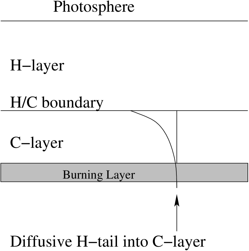
Figure 1: Diagram of a H/C envelope in diffusive equilibrium. The diffusive tail of hydrogen extends deep into the carbon, reaching temperatures where the hydrogen rapidly captures onto carbon.

In this paper, we will consider much lower values for the surface temperature, where diffusion is not the limiting step. Consider a NS envelope that consists of hydrogen above a layer of carbon (or any other proton capturing material) in diffusive equilibrium (see illustrative Figure 1). For simplicity, we do not calculate the effect of an intervening helium layer in this paper, though we estimate its possible impact in the conclusions. As long as there has been adequate time to reach a diffusive equilibrium, the separation between the hydrogen and carbon is not strict and a diffusive tail of hydrogen penetrates deep into the carbon layer. The temperature rises with depth and can increase by 1-2 orders of magnitude 10 meters beneath the photosphere. At this location, the lifetime of a proton is very short. The convolution of the increasing nuclear burning rate and the decreasing hydrogen abundance creates a burning layer at this depth, where hydrogen burning peaks. As hydrogen burns, the diffusive tail is driven slightly away from diffusive equilibrium and a diffusive current is set up, $\boldsymbol{J}_{\mathrm{DNB}}$. We will always work in the limit where $\boldsymbol{J}_{\mathrm{DNB}}$ is far less than the maximum current that can be supported due to diffusive processes so that diffusive equilibrium remains an excellent approximation.

We find that, even when the photospheric temperatures and densities are so low that the local nuclear lifetime of a proton is in excess of a Hubble time, DNB can proceed on a much faster timescale. In this paper we make some simplifying assumptions that prohibits a direct application to radio pulsars, and thus the extension of the physics to radio pulsars and magnetars will be left to future work. For example, we require a magnetic field low enough so that there is a negligible effect on the temperature profile; $B<10^{9}{\rm G}$ (Ventura & Potekhin 2002; Potekhin & Yakovlev 2001). However, our work is applicable to some X-ray transients in quiescence, where the outer envelope consists of pure hydrogen, even though the depth of the hydrogen layer is unknown.

This paper is structured as follows. In § 2 we present the basic equations and microphysics governing the thermal and compositional structure of a NS envelope in diffusive equilibrium. The derivation of the electric field strength from the envelope structure equations is in § 3. Using the derived electric field strength, we numerically solve the thermal and compositional structure of the NS envelope. The analytic solution to the NS envelope structure is given in § 4. In § 5 we discuss the relevant hydrogen burning reactions that drive the NS envelope evolution, present numerical and analytic solutions for $\boldsymbol{J}_{\mathrm{DNB}}$, and apply our theory to the X-ray transients, specifically Cen X-4. We summarize our findings in § 6.

2 Atmospheric Structure and Microphysics

We only consider the top $10^{4}\ {\rm cm}$ of the envelope, where the density is $<10^{10}\,\mathrm{\mathrm{g}\,\mathrm{cm^{-3}}}$. Since the thickness of the envelope is much smaller than the NS radius ($R\approx 10$ km), we presume a plane parallel atmosphere with a constant downward gravitational acceleration, $g=GM/R^{2}$. We neglect all relativistic corrections. The structure of the NS envelope is determined by the equations of hydrostatic balance,

$$\frac{dP_{i}}{dr} = -n_{i}\left(A_{i}m_{p}g-Z_{i}eE\right),$$ (1)

$$\frac{dP_{e}}{dr} = -n_{e}\left(m_{e}g+eE\right),$$ (2)

where $P_{i}$, $n_{i}$, $A_{i}$, $Z_{i}$ are the pressure, number density, atomic number and charge of the $i$’th ion species and $E$ is the upward pointing electric field. The thermal structure is determined by the heat diffusion equation for a constant flux, $acT_{e}^{4}/4$, where $T_{e}$ is the effective temperature,

$$\frac{dT}{dr}=-\frac{3\kappa\rho}{16T^{3}}T_{e}^{4},$$ (3)

where $\kappa$ is the opacity. Finally, we demand charge neutrality,

$$n_{e}=\sum_{i}Z_{i}n_{i}.$$ (4)

Summing the pressure equations with the charge neutrality constraint recovers the familiar form of hydrostatic balance, $dP/dr=-\rho g$.

In the outermost layers of a NS envelope, the nuclei are fully ionized and the radiative opacities are set by free-free absorption and Thomson scattering,

$$\kappa_{\rm Th}=\frac{n_{e}\sigma_{Th}}{\rho}\approx\frac{0.4}{\mu_{e}}\,\nicefrac{\mathrm{cm^{2}}}{\mathrm{g}},$$ (5)

where $\mu_{e}=A/Z$ is the electron mean molecular weight. We calculate the free-free opacity by adopting the formalism used in Schatz et al. (1999),

$$\kappa_{\rm ff}=7.53\times 10^{6}\frac{\rho_{5}}{\mu_{e}T_{6}^{7/2}}\sum\frac{Z_{i}^{2}X_{i}}{A_{i}}g_{\rm ff}(Z_{i},T,n_{e})\,\nicefrac{\mathrm{cm^{2}}}{\mathrm{g}},$$ (6)

where $T_{6}=T/10^{6}\,\mathrm{K}$, $\rho_{5}=\rho/10^{5}\,\mathrm{\mathrm{g}\,\mathrm{cm^{-3}}}$, $X_{i}$ is the mass fraction, and $g_{\rm ff}$ is the Gaunt factor. For our numerical calculations, we calculate the Gaunt factor using the Schatz et al. (1999) fitting formula [given by their equation (A2)]. For our analytic calculations we set $g_{\rm ff}=1$.

At very high densities, the dominant mode of heat transport is conduction by degenerate electrons. For strongly coupled Coulomb plasmas (SCCP), the electron thermal conductivity is determined by electron-ion scattering as given by the Wiedemann-Franz law (Ventura & Potekhin 2002; Brown, Bildsten & Chang 2002).

$$K_{c}=\frac{\pi^{2}k_{B}^{2}Tn_{e}\tau_{K}}{3m_{e}^{*}},$$ (7)

where $m_{e}^{*}=\epsilon_{\rm F}/c^{2}$ is the effective electron mass, $\epsilon_{\rm F}$ is the electron Fermi energy, and $\tau_{K}$ is the effective relaxation time. For weak magnetic fields ($B<10^{9}$G), we use the thermal conductivity of electrons in SCCP given by Baiko et al. (1998) with analytic formulae given by Potekhin et al. (1999). In the liquid metal approximation, Brown et al. (2002) showed that this formalism agrees with the calculations of Urpin & Yakovlev (1980) and Itoh et al. (1983).

The transition of the envelope from primarily radiative to primarily conductive takes place over a narrow region called the sensitivity strip (Ventura & Potekhin 2002). Heat transport by radiation and conduction is of the same order in this region. The sensitivity strip also plays the dominant role in determining the temperature profile of the NS envelope (as discussed in § 4, also see Ventura & Potekhin 2002). In the sensitivity strip, the SCCP is always in the liquid metal regime, whose conductivity is fairly well modeled (Brown et al. 2002; Ventura & Potekhin 2002). Thus, we are confident in our results for the thermal profile.

The electron equation of state transitions from an ideal gas EOS to a degenerate EOS. To model this transition in our numerical solutions, we have used the Paczynski (1983) equation of state. In our analytic calculations, we solve our envelope for the two different limits and introduce a free parameter $\Psi$ to join them at a point defined by

$$\frac{P_{\rm e,deg}}{P_{\rm e,nondeg}}\equiv\Psi,$$ (8)

where $P_{\rm e,deg}$ and $P_{\rm e,nondeg}$ are the nonrelativistic degenerate and nondegenerate electron equations of state respectively. For this calculation we take $\Psi=1.5$, which gives a reasonable approximation to the full numerical solution in the region of the envelope where DNB occurs.

3 Elemental Distribution and Electric Field Strength

The composition of the envelope in diffusive equilibrium is found by simultaneously solving the equations of hydrostatic balance for each species and the flux equation. This approximation is excellent once enough time has passed for the diffusive equilibrium to be established (Brown et al. 2002).

We begin by calculating the local electric field. In early studies of white dwarfs and NSs (Rosen 1968; Fontaine & Michaud 1979), the electric field was presumed to be that for an ideal gas of ions and electrons,

$$eE=\frac{A}{Z+1}m_{p}g.$$ (9)

However, in the degenerate case where $P_{e}\approx P$, the field is

$$eE=\frac{A}{Z}m_{p}g.$$ (10)

These results are only valid in certain limits, where the plasma consists of one dominant species and where the gas is either very degenerate or very non-degenerate. For multi-ion plasmas and for partial degeneracy, these simple approximations break down. For a more general solution, we calculate the electric field from the ion and electron equations of hydrostatic balance (eq. [1]), and the flux equation (eq. [3]). We presume an ideal gas equation of state for the ions and an arbitary electron equation of state. Finally we drop the $m_{e}g$ term.

Let us first consider the isothermal case. We first expand $\partial P_{e}/\partial r$,

$$\frac{\partial n_{e}}{\partial r}=-\left(\frac{\partial P_{e}}{\partial n_{e}}\right)^{-1}n_{e}eE,$$ (11)

and then use the ideal gas equation of state for the ions:

$$\frac{\partial n_{i}}{\partial r}=-\frac{n_{i}}{kT}(A_{i}m_{p}g-eZ_{i}E).$$ (12)

Multiplying each ion equation (eq. [12]) by $Z_{i}$ and subtracting their sum from the electron equation (eq. [11]) and presuming charge neutrality (eq. [4]) gives

$$eE=\frac{m_{p}g\sum n_{i}A_{i}Z_{i}}{\sum n_{i}Z_{i}^{2}+n_{e}k_{B}T\left({\partial P_{e}}/{\partial n_{e}}\right)^{-1}}.$$ (13)

For the nonisothermal case, we get an additional term in the expansion of $\partial P_{e}/\partial r$ and $\partial P_{i}/\partial r$, e.g.

$$\frac{\partial n_{e}}{\partial r}=-\left(\frac{\partial P_{e}}{\partial n_{e}}\right)^{-1}\left(n_{e}eE-\frac{\partial P_{e}}{\partial T}\frac{\partial T}{\partial r}\right),$$ (14)

and the electric field becomes

$$eE=\frac{\sum n_{i}Z_{i}\left(A_{i}m_{p}g+k_{B}\left({dT}/{dr}\right)\right)-\left({\partial P_{e}}/{\partial T}\right)\left({\partial P_{e}}/{\partial n_{e}}\right)^{-1}\left({dT}/{dr}\right)}{\sum n_{i}Z_{i}^{2}+n_{e}k_{B}T\left({\partial P_{e}}/{\partial n_{e}}\right)^{-1}}.$$ (15)

This result agrees with the results of Macdonald, Hernanz & Jose (1998) and Althaus & Benvenuto (2000), but we have decoupled our solution of the electric field from the drift velocity and diffusion coefficient. Hence, the electric field is simply a function of local parameters. For the purposes of numerical calculation we use the Paczynski (1983) electron equation of state. For our analytic calculations, we use either the ideal gas or the nonrelativistic degenerate electron equation of state depending on the local conditions of the plasma.

At this point, it is helpful to illustrate a solution for the particular case of a $\mathrm{H}$/$\mathrm{{}^{12}C}$ envelope. In Figure 2, we plot the electric field of the layer as a function of column depth, $y=P/g$. We integrate from the photosphere with a background of $\mathrm{H}$. At a certain depth we introduce a low carbon abundance and continue integrating inward. As expected, the electric field approximates that of the value given by equation (9) at the extreme limits where one ion dominates over the other. The slight discrepancy between the value give by equation (9) at the extreme limits is due to degeneracy effects from the Paczynski (1983) fit of the electron equation of state. The flux and structure equations can now be solved self consistently to model any arbitrary envelope in diffusive equilibrium. In Figure 3, we plot the solution for a $\mathrm{H}$/$\mathrm{{}^{12}C}$ envelope. We plot the composition profile in terms of the concentration of hydrogen, $f_{H}=n_{H}/n_{t}$, where $n_{t}$ is the total number of ions.

4 Approximate Solutions for Temperature and Composition

The temperature and composition profiles can be represented well with approximate analytic solutions that illuminate the physics. Hernquist & Applegate (1984) and Ventura & Potekhin (2002) have presented analytic thermal calculations of the NS envelope, but their solutions are too complex for our analytic estimates. Hence, we present simplified approximate solutions in § 4.1. For an envelope in diffusive equilibrium, Fontaine & Michaud (1979) have presented an excellent approximate solution for the composition profile. In § 4.2, we extend their technique to the degenerate regime.

4.1 Analytic Temperature Profile

Roughly speaking, the NS envelope can be divided into three zones, a radiative outer zone, a sensitivity strip (where opacity changes from primarily radiative to conductive), and a conductive isothermal interior (also see Ventura & Potekhin 2002). In the radiative, nondegenerate outer zone, the opacity is mostly determined by free-free absorption. With an ideal gas equation of state, $yg=\rho k_{B}T/\mu m_{p}$, where $\mu=A/(Z+1)$ is the mean molecular weight of the plasma, the solution to the heat diffusion equation and hydrostatic balance is

$$T(y)=1.58\times 10^{6}y^{4/17}\left(\mu Zg_{14}T_{e6}^{4}\mu_{e}^{-2}\right)^{2/17}\,\mathrm{K},$$ (16)

where for brevity we have written $g_{14}=g/(10^{14}\,\mathrm{cm}\,\mathrm{s}^{-2})$ and $T_{e6}=T_{e}/(10^{6}\,\mathrm{K})$. For a radiative nondegenerate envelope consisting of multiple layers of ions, the solution is modified via the introduction of constants of integration at the boundaries. If the boundaries are sufficiently far away in pressure from the sensitivity strip, the temperature profile of the underlying layers will approximate that of a pure component.

In the sensitivity strip, which is defined by $\kappa_{\rm rad}(y_{\rm ss})=\kappa_{\rm cond}(y_{\rm ss})$, the opacity transitions from primarily radiative to primarily conductive. Here we follow the formalism of Ventura & Potekhin (2002). To find the sensitivity strip, we take the approximate expression for conductivity (Ventura & Potekhin 2002),

$$K_{c}=2.3\times 10^{15}\frac{T_{6}}{\Lambda Z}\frac{\chi^{3}}{1+\chi^{2}}\frac{\rm ergs}{\,\mathrm{cm}\,\mathrm{s}\,\mathrm{K}},$$ (17)

where $\chi=p_{F}/m_{e}c\approx(\rho_{6}/\mu_{e})^{1/3}$ is the relativity parameter, $\mu_{e}=A/Z$, and $\Lambda$ is the Coulomb logarithm. We set $\Lambda=1$ for simplicity’s sake and $1+\chi^{2}\approx 1$ since the relativity parameter is small in the nonrelativistic regime. Equating the two opacities, equations (6) and (17), we find that the sensitivity strip is defined by the condition,

$$y=11.2\frac{A^{1/3}T_{6}^{17/6}\mu_{e}^{2/3}}{Z^{1/3}g_{14}\mu}\,\nicefrac{\mathrm{g}}{\mathrm{cm^{2}}}.$$ (18)

Taking this condition and inserting the solution for the radiative zone, we obtain expressions for the column depth of the sensitivity strip, $y_{\rm ss}$,

$$y_{\rm ss}=6.86\times 10^{4}\frac{ZT_{e6}^{4}\mu_{e}}{g_{14}^{2}\mu^{2}}\,\nicefrac{\mathrm{g}}{\mathrm{cm^{2}}},$$ (19)

and temperature,

$$T_{\rm ss}=2.2\times 10^{7}\left(\frac{Z^{3}T_{e6}^{12}}{g_{14}^{3}\mu^{3}}\right)^{2/17}\,\mathrm{K},$$ (20)

as a function of effective temperature, gravity, and composition. Beyond the sensitivity strip ($y>y_{\rm ss}$), we solve the constant flux equation using the conductive opacity,

$$T\frac{dT}{dy}=2.2\times 10^{16}\frac{ZT_{e6}^{4}\mu_{e}}{\rho^{2}},$$ (21)

when $1+\chi^{2}\approx 1$. Integration of this equation is relatively straightforward given an equation of state. There are two cases that we need to consider. For the nondegenerate regime, the solution for $y>y_{\rm ss}$ is

$$T=T_{\rm ss}\exp\left[-1.62\times 10^{4}\frac{Z\Lambda T_{e6}^{4}\mu_{e}}{g_{14}^{2}\mu^{2}}\left(y^{-1}-y_{\rm ss}^{-1}\right)\right]\,\mathrm{K},$$ (22)

where we have joined it with the radiative solution at the sensitivity strip.

The electrons become more degenerate as the column increases. We define the degenerate boundary with our analytic degeneracy condition (eq. [8]), which gives the condition

$$y=22\frac{T_{6}^{5/2}\Psi^{5/2}\mu_{e}^{5/3}}{g_{14}\mu^{5/2}}\,\nicefrac{\mathrm{g}}{\mathrm{cm^{2}}},$$ (23)

where we have assumed that $y_{\rm deg}\gg y_{\rm ss}$. Using our solution for $T$ beyond the sensitivity strip (eq. [22]), we find a system of equations for $T_{\rm deg}$ and $y_{\rm deg}$, which are solved numerically.

The solution beyond the degenerate boundary is

$$T^{2}-T_{\rm deg}^{2}=1.37\times 10^{16}T_{e6}^{4}\frac{Z}{g_{14}^{6/5}\mu_{e}}\left(y_{\rm deg}^{-1/5}-y^{-1/5}\right)\,\mathrm{K}^{2}.$$ (24)

Taking the limit of equation (24) as $y\rightarrow\infty$ gives an analytic expression for the core temperature, $T_{c}$, as a function of $T_{e}$, which reproduces previous scalings (Gudmundsson, Pethick & Epstein 1983; Potekhin, Chabrier & Yakovlev 1997). Ventura & Potekhin (2002) present a more generalized solution in terms of the relativity parameter $\chi$.

In Figure 3 we present the approximate and numerical solutions for the temperature and composition which we discuss in the next section. For the thermal profile, the agreement is excellent (to within 10%). It also agrees well with the analytic solution given by Ventura & Potekhin (2002).

4.2 Analytic Composition Profiles

We find analytic solutions for the composition when one ion species is dominant and the electrons are either nondegenerate or very degenerate. For the nondegenerate case, we first derive the result of Fontaine & Michaud (1979). We start with the hydrostatic balance equations for the ions, where “1” is the background and “2” is the trace,

$$\frac{dP_{1}}{dr}=-n_{1}\left(A_{1}m_{p}g-Z_{1}eE\right),$$ (25)

$$\frac{dP_{2}}{dr}=-n_{2}\left(A_{2}m_{p}g-Z_{2}eE\right).$$ (26)

For the ions, $P_{i}=n_{i}k_{B}T$. Dividing each pressure equation above by their respective $P_{i}$ and subtracting “1” from “2”, we have:

$$k_{B}T\frac{d\ln\left(P_{2}/P_{1}\right)}{dr}=-\left(A_{2}-A_{1}\right)m_{p}g+\left(Z_{2}-Z_{1}\right)eE,$$ (27)

which in the trace limit ($n_{2}\ll n_{1}$) gives

$$\ln\left(\frac{P_{2}}{P_{1}}\right)=\ln\left(\frac{n_{2}}{n_{1}}\right)\approx\ln\left(\frac{n_{2}}{n_{1}+n_{2}}\right)=\ln f_{2},$$ (28)

where $f_{2}$ is number fraction of the trace.

In the nondegenerate regime, the electric field is given by equation (9). Using this result and using the trace approximation so that $A\approx A_{1}$ and $Z\approx Z_{1}$, equation (27) becomes

$$\frac{d\ln f_{2}}{dr}=-\frac{A_{1}m_{p}g}{(Z_{1}+1)k_{B}T}\left[\frac{A_{2}}{A_{1}}(Z_{1}+1)-Z_{2}-1\right]$$ (29)

Using hydrostatic balance $dP/dr=-\rho g\approx-A_{1}m_{p}gn_{1}$ and $P\approx(Z_{1}+1)n_{1}kT$, we have the elegant result,

$$\frac{d\ln f_{2}}{d\ln P}=\left[\frac{A_{2}}{A_{1}}(Z_{1}+1)-Z_{2}-1\right].$$ (30)

The concentration of a trace species is a power law of pressure with an exponent, $\delta=A_{2}(Z_{1}+1)/A_{1}-Z_{2}-1$. It is widely applicable because it gives the concentration in terms of a pressure contrast,

$$f_{2}(P)=f_{2}(P_{\rm b})\left(\frac{P}{P_{\rm b}}\right)^{\delta},$$ (31)

where $f_{2}(P_{\rm b})$ is the concentration at an arbitrary boundary $P_{\rm b}$.

We now extend this result to the highly degenerate regime, where the electron pressure dominates over ion pressure, and the electric field is

$$eE=\frac{m_{p}g}{\mu_{e}}=\frac{A}{Z}m_{p}g.$$ (32)

Placing this into equation (27) gives

$$\frac{d\ln f_{2}}{dP}=\frac{A_{1}m_{p}}{\rho(P,T)k_{B}T(P)}\left[\frac{A_{2}}{A_{1}}-\frac{Z_{2}}{Z_{1}}\right].$$ (33)

We solve for $\rho(P,T)$ via the electron equation of state and $T(P)$ from the flux equation. This solution is best when the electrons are highly degenerate. However, this is also the regime where the temperature begins to be isothermal (Ventura & Potekhin 2002), allowing us to replace $T(P)$ by $T_{\rm deg}$, where $T_{\rm deg}$ is the temperature at the degenerate boundary, giving

$$\frac{d\ln f_{2}}{dP}=\frac{A_{1}m_{p}}{\rho_{\rm deg}\left(P/P_{\rm deg}\right)^{1/\gamma}k_{B}T_{\rm deg}}\left[\frac{A_{2}}{A_{1}}-\frac{Z_{2}}{Z_{1}}\right],$$ (34)

where $\gamma$ is the polytropic index of the degenerate electron equation of state, $P\varpropto\rho^{\gamma}$. The condition of degeneracy (eq. [8]) determines $P_{\rm deg}$ and $\rho_{\rm deg}$.

The electrons are nonrelativistic at the degenerate boundary so $\gamma=5/3$ and we integrate (eq. [34]) to get

$$f_{2}=f_{\rm 2,deg,0}\exp\left\{-\eta\frac{A_{1}m_{p}P_{\rm deg}}{\rho_{\rm deg}k_{B}T_{\rm deg}}\left[\frac{Z_{2}}{Z_{1}}-\frac{A_{2}}{A_{1}}\right]\left[\left(\frac{P}{P_{\rm deg}}\right)^{\eta}-1\right]\right\}$$ (35)

where $f_{\rm 2,deg,0}$ is the concentration where the envelope becomes degenerate and $\eta=1-\frac{1}{\gamma}=0.4$. Note that $\eta$ is positive for all degenerate equations of state: the concentration always decreases exponentially with increasing pressure. Our solution reproduces the Boltzmann solution for a particle experiencing a upward pointing force $F$ in the isothermal limit, $f_{2}\varpropto\exp\left(Fr/kT\right)$ since $r\varpropto P/\rho\varpropto P^{\eta}$. Thus, in the degenerate regime the concentration falls faster than the power law relation in the nondegenerate regime. In Figure 3, we compare the numerical solution with our analytic calculation. The agreement is poor for higher densities due to the increasing importance of relativistic equation of state, but gives reasonable agreement in the burning layer $y_{\rm burn}\sim 10^{6}\,\mathrm{\mathrm{g}\,\mathrm{cm^{-2}}}$.

5 Hydrogen Burning in Diffusive Equilibrium

The relevant nuclear processes that consume hydrogen depend on the temperature and composition of the underlying matter. We consider the case of a NS which has a pure hydrogen layer on top of a layer of proton capturing material (i.e. carbon, nitrogen, oxygen, etc) in diffusive equilibrium. We have not yet calculated the impact of an intervening He layer, but we think it will be small as long as it does not penetrate to a depth greater than the burning layer.

For simplicity, we first consider carbon. For hydrogen on carbon, there are only two possible nuclear reactions: $\mathrm{{}^{12}C}({\rm p},\gamma)\mathrm{{}^{13}N}$ and ${\rm p}({\rm p},e^{+}+\nu_{e}){\rm D}$. The D produced in the p-p capture undergoes ${\rm D}({\rm p},\gamma)\mathrm{{}^{3}He}$ which in general is the endpoint of this process. Since we always have a region where T $>10^{7}\,\mathrm{K}$, the reaction rate for p-p capture is very slow compared to the proton capture rate onto carbon. The $\mathrm{{}^{13}N}$ decays to $\mathrm{{}^{13}C}$ which has $A/Z=13/6\approx 2.167$, greater than the local $A/Z=2$ for pure carbon. The $\mathrm{{}^{13}C}$ will thus sink through the outer layers of the NS, and will not reside long enough in the burning layer to facilitate a catalytic cycle. Hence, the complete exhaustion of $\mathrm{H}$ by this process requires an excess of $\mathrm{{}^{12}C}$ compared to $\mathrm{H}$.

5.1 Diffusive Nuclear Burning

We calculate the burning rate presuming that the burning time is slow compared to the time for hydrogen to diffuse down through the carbon to the burning layer. We express this hierarchy of diffusion time to nuclear burning time by studying the $\mathrm{H}$ equation of continuity,

$$\frac{\partial n_{H}}{\partial t}+\boldsymbol{\nabla\cdot{\boldsymbol{J}}}_{H}=-\frac{n_{H}}{\tau_{H}},$$ (36)

where $\tau_{H}=\langle\sigma v\rangle^{-1}n_{C}^{-1}$ is the local lifetime of $\mathrm{H}$ to $\mathrm{{}^{12}C}$ capture. The condition of diffusive equilibrium is $\partial n_{H}/\partial t=0$ or more specifically that $\partial n_{H}/\partial t$ changes only on the timescale associated with depletion of the hydrogen column, which is long compared to both the local nuclear burning time $\tau_{H}$ and the diffusion time and therefore is dropped. With the condition of steady state $\boldsymbol{J}_{H}$ and $\boldsymbol{J}_{\mathrm{DNB}}$ are equivalent. Writing the result in one dimension for $\boldsymbol{J}_{H}=\boldsymbol{J}_{\mathrm{DNB}}=\mathcal{D}\partial n_{H}/\partial z-n_{H}v_{\rm dr}$, we have

$$\mathcal{D}\frac{\partial^{2}n_{H}}{\partial z^{2}}-v_{\rm dr}\frac{\partial n_{H}}{\partial z}=-\frac{n_{H}}{\tau_{H}},$$ (37)

, where $\mathcal{D}$ is the diffusion coefficient and $v_{\rm dr}$ is the drift velocity. We presume that $\mathcal{D}$ and $v_{\rm dr}$ change slowly with $z$. Our presumption that nuclear burning does not affect diffusive equilibrium implies that locally the timescale associated with nuclear burning is much longer than the timescale associated with diffusion to the burning layer, or $\tau_{H}\gg\tau_{\rm ion}=l^{2}/\mathcal{D}$, where $l$ is the ion scale height for $\mathrm{H}$in the $\mathrm{{}^{12}C}$ layer. Therefore, taking $\mathcal{D}$ from Brown et al. (2002), we have

$$\tau_{\rm ion}=800\frac{T_{6}^{0.7}Z_{i}^{1.3}\rho_{5}^{0.6}}{A_{i}^{0.1}g_{14}^{2}\left(A_{i}-Z_{i}\right)^{2}}\,\mathrm{s},$$ (38)

where $A_{i}$ and $Z_{i}$ are the atomic number and charge of the background proton capturing element.

For proton capturing reactions, the proton lifetime (Clayton 1983) is

$$\tau_{\rm H}^{-1}=2.45\times 10^{16}\left(\frac{S_{0}}{1\,{\rm keV}\,{\rm barns}}\right)\frac{\rho X_{i}}{A_{i}}T_{6}^{-2/3}\exp\left(-BT_{6}^{-1/3}\right)\,\mathrm{yrs}^{-1}$$ (39)

where $X_{i}$ and $A_{i}$ is the mass fraction and atomic number of the proton capturing element and $S_{0}$ and $B$ are parameters determined by the proton capturing element. We derive an analytic expression for the condition of diffusive equilibrium by expanding equation (39) about $T_{6}=40$,

$$\tau_{H}=1.32\times 10^{5}\rho_{5}^{-1}\left(\frac{T_{6}}{40}\right)^{-14}\,\mathrm{s}.$$ (40)

Comparing equations (38) and (40), our condition for carbon is

$$T_{6}<45.5\rho_{5}^{-0.11},$$ (41)

for $g_{14}=2$.

If the conditions for DNB are fulfilled for a sufficiently large pressure range, the total burning rate of hydrogen, defined as $\zeta_{H}=\boldsymbol{J}_{\mathrm{DNB}}({\rm H/\mathrm{{}^{12}C}\ boundary})$ is

$$\zeta_{H}=\frac{y_{H}}{\tau_{\rm col}}=\int\frac{n_{H}m_{p}}{\tau_{H}(n_{H},n_{C},T)}dz,$$ (42)

where $y_{H}$ is the integrated column of hydrogen, $\tau_{\rm col}$ is the characteristic time for that column to be consumed and $n_{H}$ and $n_{C}$ are the local number density of hydrogen and carbon respectively. This equation is incorporated into our flux and structure equations and solved simultaneously, yielding $\tau_{\rm col}$ as a function of our stellar properties and $y_{H}$. We plot $d\zeta_{H}/d\lg_{10}y$ for an envelope with $y_{H}=100\,\mathrm{\mathrm{g}\,\mathrm{cm^{-2}}}$ in Figure 4. In the bottom graph we show the local concentration and temperature. Due to the inverse dependence of the local hydrogen burning rate on temperature and concentration, the burning layer is concentrated in a narrow pressure range at a depth where the $\mathrm{H}$ abundance is small. The diffusion timescale to this depth is $\tau_{\rm ion}=10^{4}\,\mathrm{s}$, which is much shorter than the nuclear timescale of $1.5\times 10^{7}\,\mathrm{s}$. This observation is the essence of DNB, namely, that practically all the burning occurs in the exponentially suppressed diffusive hydrogen tail.

In Figure 5, we plot the characteristic time, $\tau_{\rm col}$, and characteristic mass burning rate, $\dot{M}_{\rm DNB}=4\pi R^{2}y_{H}/\tau_{\rm col}$, for $g_{14}=2$ and fixed core temperature, $T_{c}$. For a central temperature of $5\times 10^{7}\,\mathrm{K}$, our calculations are valid only up to $3\times 10^{7}\,\mathrm{\mathrm{g}\,\mathrm{cm^{-2}}}$. Above this column, the assumption of constant flux breaks down since the energy released from DNB is comparable to the flux.

Two results are obvious from this figure. First the relation between lifetime (and hence mass burning rate) and column is related via a simple power law between $\tau_{\rm col}$ and $y_{H}$. We derive this power law in § 5.2. Secondly, the lifetime of the entire envelope is set by the lifetime of the photosphere.

The location of the burning layer must satisfy our derived diffusive equilibrium condition, (eq. [41]) for our calculation to be valid. In Figure 6, we plot various models against our condition for DNB in diffusive equilibrium (eq. [41]). The burning layers is the region between the two vertical lines in each model. For models with $T_{e}>10^{6}\,\mathrm{K}$ (or $T_{c}>6\times 10^{7}\,\mathrm{K}$), our present calculation is not valid as DNB will occur in the slow diffusion limit. We will expand on this point and study the slow diffusion limit in a future paper.

5.2 Approximate Solution

The competition between the falling $\mathrm{H}$ abundance and rising temperature with depth forces much of the hydrogen burning to occur in a narrow zone. As a result, we can solve the burning integral (eq. [42]) over the burning layer by approximating it with the method of steepest descents.

Since DNB occurs deep below the hydrogen layer, $X_{i}\approx 1$, equation (42) then becomes

$$\zeta_{H}=\frac{y_{H}}{\tau_{\rm col}}=2.45\times 10^{16}A_{i}^{-2}\left(\frac{S_{0}}{1\,{\rm keV}\,{\rm barns}}\right)\int{\rho}yf_{H}T_{6}^{-2/3}\exp\left(-BT_{6}^{-1/3}\right)d\ln(y)\,\mathrm{yrs}^{-1}$$ (43)

where $f_{H}$ is the local number concentration of hydrogen, which decreases with increasing $y$. Note that we have made a change of variables of $dz=y\rho^{-1}d\ln(y)$.

This integral should be evaluated in both the nondegenerate, radiative regime and the degenerate, conductive regime. However, since the majority of the burning occurs in the degenerate, conductive regime, we will evaluate the integral there by the method of steepest descents (Clayton 1983),

$$\int g(x)\exp(-h(x))dx\approx g(x_{0})\exp(-h(x_{0}))\sqrt{\frac{2\pi}{h^{\prime\prime}(x_{0})}},$$ (44)

where $g(x)$ is a slowly varying function function of $x$, $h(x)$ is a peaked function, and $x_{0}$ is the solution of $h^{\prime}(x_{0})=0$, the location of the peak of the burning rate. In order to carry out this approximation for equation (43), we make the following identifications,

$$\exp(-h(x)) \rightarrow y\rho f_{H}\exp\left(-BT_{6}^{-1/3}\right),$$

$$g(x) \rightarrow T_{6}^{-2/3}.$$ (45)

For the degenerate, conductive regime, the peaked function is

$$-h\left[\ln(y)\right]=\frac{8}{5}\ln(y)-BT_{6}^{-1/3}-\eta\frac{A_{i}m_{p}gy_{\rm deg}}{\rho_{\rm deg}k_{B}T_{\rm deg}}\left(\frac{1}{Z_{i}}-\frac{1}{A_{i}}\right)\left[\left(\frac{y}{y_{\rm deg}}\right)^{-\eta}-1\right].$$ (46)

The last term comes from the analytic solution for the composition profile (eq. [35]), where the background is the proton capturing element and the trace is hydrogen. The temperature, $T$, in the degenerate regime is given by equation (24). Since the burning peak $y_{0}$ is defined by a transcendental equation, $h^{\prime}(\ln(y_{0}))=0$, we solve it numerically and then calculate $h^{\prime\prime}(\ln(y_{0}))$. For a total column of hydrogen of $y_{H}=100\,\mathrm{\mathrm{g}\,\mathrm{cm^{-2}}}$, $T_{e}=8\times 10^{5}\,\mathrm{K}$, and $g_{14}=2$, we find by the method of steepest descents, $\tau_{\rm col}=468\,\mathrm{yrs}$, which compares well with the numerical answer of $\tau_{\rm col}=428\,\mathrm{yrs}$. The burning layer is centered around $y_{0}=7.2\times 10^{5}\,\mathrm{\mathrm{g}\,\mathrm{cm^{-2}}}$ with a local temperature of $T(y=y_{0})=2.6\times 10^{7}\,\mathrm{K}$ and central core temperature $T_{c}=3.3\times 10^{7}\,\mathrm{K}$.

Power law scalings of $\tau_{\rm col}$ with $y_{H}$, $T_{e}$ and $g$ can also be determined from this integral. The simplest power law scaling involves $y_{H}$, which we determine as follows. The rate, $y_{H}/\tau_{\rm col}$, is directly proportional to $f_{H}$ as in equation (43). From equation (31) and (35), $f_{H}\varpropto f_{\rm H,deg,0}=(y_{\rm deg}/y_{H})^{\delta}$, where $f_{\rm H,deg,0}$ is the hydrogen number fraction at the degenerate boundary and $\delta=A_{2}(Z_{1}+1)/A_{1}-Z_{2}-1=-17/12$ for H on $\mathrm{{}^{12}C}$. Therefore, $\tau_{\rm col}\varpropto y_{H}^{1+\delta}$, which is confirmed from comparisons to the numerical results. This scaling is accurate as long as $y_{H}<y_{\rm deg}$.

The scaling of $\tau_{\rm col}$ against $T_{e6}$ and $g_{14}$ can be derived from a power-law expansion of burning integral (eq. [43]) in terms of $T$. The expansion of the burning integral (eq. [43]) gives

$$\frac{y_{H}}{\tau_{\rm col}}\varpropto f_{H}T_{0,6}^{-2/3}\exp\left(-BT_{0,6}^{-1/3}\right),$$ (47)

where $T_{0,6}=T_{0}/10^{6}$ and $T_{0}$ is the temperature of the burning layer. Since we are in the degenerate conductive regime, $T_{0}\approx T_{c}$. The location of the burning region, $y_{0}$ and $\rho_{0}$, scale weakly with $T$ compared to the temperature of the burning region, $T_{0}$. Taking the analytic solution to the temperature profile (eq. [24]) and degeneracy point (eq. [23]), the power law dependence between $T_{c}$, $T_{e6}$ and $g_{14}$ is $T_{0}\varpropto T_{c}\varpropto T_{e6}^{2}g_{14}^{-1/2}$. Therefore, the scaling of $f_{H}$ in $\mathrm{{}^{12}C}$ goes as,

$$f_{H}\varpropto\exp\left\{-\eta\frac{m_{p}P_{\rm deg}}{\rho_{\rm deg}k_{B}T_{0}}\left[\left(\frac{P}{P_{\rm deg}}\right)^{-\eta}-1\right]\right\}.$$ (48)

Expanding this equation at $T_{0}=10^{8}K$ gives $f_{H}\varpropto(T_{0}/10^{8})^{0.475}g_{14}^{0.285}\varpropto T_{e6}^{0.95}g_{14}^{0.0475}$. Expanding the exponential in equation (47) for carbon ($B=136.96$) gives $\exp\left(-BT_{c}^{-1/3}\right)\varpropto T_{c}^{9.8}\varpropto T_{e6}^{19.7}g_{14}^{-4.9}$. Thus, the scaling for the rate is ${y_{H}}/{\tau_{\rm col}}\varpropto T_{e6}^{19.3}g_{14}^{-4.52}$. Hence, the dominant scaling comes from the exponential dependence on temperature of the nuclear burning rate with small corrections from the other factors. Putting all the scalings together with our analytic calculation, we find

$$\tau_{\rm col}\approx 6.5\left(\frac{y_{H}}{100\,\mathrm{\mathrm{g}\,\mathrm{cm^{-2}}}}\right)^{-5/12}T_{e6}^{-19.3}\left(\frac{g_{14}}{2}\right)^{4.52}\,\mathrm{yrs}.$$ (49)

In Figure 7, we compare the scaling found numerically with this analytic result and find reasonable agreement. The agreements for the scalings of $y_{H}$ and $g_{14}$ and the numerical results are good. However, the agreement for the scaling of $T_{e}$ and numerical results diverge for low $T_{e}$. This is due to the changing power law with respect to expanding around different values of $T_{c}$. Expanding around a value of $T_{c}$ appropriate for these lower values of $T_{e}$ resolves this discrepancy.

These scalings can be calculated for other proton capturing elements. The scaling of $\tau_{\rm col}$ and $y_{H}$ remains the same with the exponent $1-\delta_{i}$, where $\delta_{i}$ takes on different values for the differing backgrounds $(Z_{i},\ A_{i})$. We can use the same strategy as earlier, expanding our results in $T_{0}$ and inserting the scalings for $T_{e6}$ and $g_{14}$ afterwards. Hence, $f_{H}$ has the same scaling as before, $f_{H}\varpropto(T_{0}/10^{8})^{0.475}g_{14}^{0.285}$. However, the dominant scaling from the exponential dependence of temperature on the burning rate changes. Hence we choose to ignore the scalings associate with $f_{H}$. In terms of the exponential factor $B_{i}$, this dependence becomes $\exp\left(-B_{i}T_{0,6}^{-1/3}\right)\varpropto\left({T_{0}}/{10^{8}\,\mathrm{K}}\right)^{B_{i}/14}\varpropto T_{e6}^{B_{i}/7}g_{14}^{-B_{i}/28}$. Since $f_{H}$ does not scale strongly with $T_{0}$ compared to the nuclear reaction rate (especially with heavier elements where $B_{i}$ gets progressively larger), we ignore the scaling of $f_{H}$ with $T_{0}$ and $g_{14}$. To put this another way, the value of the number density, $f_{H}$, at the burning layer does not change as drastically as the value of the nuclear timescale at the burning layer with $T_{0}$. Putting these scalings all together, we have

$$\tau_{\rm col_{i}}=\tau_{\rm col_{i},0}\left(\frac{y_{H}}{100\,\mathrm{\mathrm{g}\,\mathrm{cm^{-2}}}}\right)^{1+\delta_{i}}T_{e6}^{-B_{i}/7}g_{14}^{B_{i}/28},$$ (50)

Table 1 lists the values of the scalings, the prefactor, calculated both numerically and analytically, and the largest effective temperature where DNB in diffusive equilibrium is valid. Above $T_{e,6\,\mathrm{DNB}}$, equation (50) is not valid since DNB no longer occurs in diffusive equilibrium.

5.3 Application to Cen X-4 in Quiescence

The large number of transiently accreting NS also provide an astrophysical site for our work. The work of Rutledge et al. (1999) (see Bildsten and Rutledge 2001 for an overview) first showed that much of the quiescent emission from these objects was thermal emission from the surface, allowing for many $T_{e}$ measurements (Rutledge et al. 2001a, b, 2000, 1999). Of all these LMXBs, only Cen X-4 is safely in the DNB regime. Its effective temperature is low enough ($T_{e}=8.8\times 10^{5}$ Rutledge et al. 2001a) so that DNB in diffusive equilibrium is a good approximation for a hydrogen column $y_{H}<10^{8}\,\mathrm{\mathrm{g}\,\mathrm{cm^{-2}}}$. The column depth of H on Cen X-4 after an outburst is expected to be $y_{H}<10^{8}\,\mathrm{\mathrm{g}\,\mathrm{cm^{-2}}}$; set by ignition conditions of type I X-ray bursts (Brown et al. 2002).

Accretion outbursts were observed in 1969 and 1979 from Cen X-4, but the latter outburst was particularly weak. Presuming no outburst has occurred in the intervening years, this gives an age of 23 years. For a hydrogen column of $y_{H}=10^{8}\,\mathrm{\mathrm{g}\,\mathrm{cm^{-2}}}$ after the 1979 outburst, we find that the present parameters of Cen X-4 would be $y_{H}\approx 2\times 10^{6}\,\mathrm{\mathrm{g}\,\mathrm{cm^{-2}}}$ and $T_{c}\approx 4\times 10^{7}$ K if there has been no accretion in quiescence. A much larger H column ($y_{H}\approx 2\times 10^{7}\,\mathrm{\mathrm{g}\,\mathrm{cm^{-2}}}$) is needed to burn matter via DNB at the supplied rate if the NS is accreting in quiescence at a rate $\dot{M}_{q}=10^{-13}M_{\odot}\,{\rm yr}^{-1}$.

Presuming little accretion in quiescence and fixed $T_{c}$, we evolve $y_{H}$ and the resulting flux as a function of the time since the last outburst. The age of the envelope or time since the last outburst, $t_{\rm age}$ is the age derived from the scaling of $\tau_{\rm col}$ with $y_{H}$ in the analytic solution,

$$t_{\rm age}=\int\left(\frac{dy_{H}}{dt}\right)^{-1}dy_{H}=\frac{12}{5}\tau_{\rm col}.$$ (51)

In Figure 8, we plot the resultant flux from a total integrated column of $\mathrm{H}$, $y_{H}$, against the lifetime of that column for fixed core temperature, $T_{c}$. Evolution via DNB predicts that the outgoing flux will drop by $\sim 12\%$ over a twenty year period roughly 100 years after the outburst. This drop is due to the consumption of $\mathrm{H}$ that makes up the sensitivity strip of the $\mathrm{H}$ layer. At present (twenty years after the outburst) the flux will vary by only 3% over a ten year timescale. The associated $\dot{M}_{\rm DNB}=2\times 10^{-15}M_{\odot}\,{\rm yr}^{-1}$ for this time after the outburst. Observations of Cen X-4 have placed constraints on the variation of $T_{e}$ over a five year timescale of $<10\%$ (Rutledge et al. 2001a). Observational confirmation of DNB on Cen X-4 is therefore unlikely.

6 Conclusions and Discussions

We have shown that diffusive nuclear burning (DNB) is an effective mechanism that burns surface hydrogen on a NS on astrophysically relevant timescales. Our numerical and analytic solutions for the rates of DNB are in the limit where the H is in diffusive equilibrium with the underlying proton capturing elements. Our work is similar to that originally carried out by Michaud and Fontaine (Michaud et al. 1984; Michaud & Fontaine 1984) for diffusion-induced hydrogen burning in white dwarfs and also by Iben & MacDonald (1985a, b). However, there are several crucial differences: the NS temperatures are much higher and the local gravity much stronger. Hence, we were able to make simplifying assumptions and avoid the active diffusion calculation with nuclear burning performed by Iben & MacDonald (1985a). We have also solved for the concentration profile in the degenerate regime self-consistently, whereas the effects of degeneracy were neglected in Michaud and Fontaine’s paper.

The largest remaining uncertainty in applying our work is the unknown composition of the material underlying the hydrogen. Our assumptions of low magnetic fields and surface temperatures ($T_{e}<10^{6}\ {\rm K}$ for DNB to be nuclear-rate limited) limit the DNB applications to quiescent NSs in transient low-mass X-ray binaries and millisecond radio pulsars. Little is known about the surface composition of millisecond radio pulsars, though in the absence of our work one would definitely expect H to be dominant on the surface since these objects underwent mass accretion prior to becoming a pulsar. If there is enough carbon in the underlying composition from previous H/He burning during type I X-ray bursts (Schatz et al. 1999), then there is clearly adequate time to burn off the H. A clear detection of H at the photosphere of a millisecond radio pulsar would thus constrain the underlying abundances.

The impact of an intervening helium layer depends on its thickness. A thin layer of helium, which does not penetrate into the burning layer and remains in the nondegenerate regime, enhances the burning rate. This is because the electric field in a nondegenerate helium plasma ($E=4m_{p}g/3e$) is smaller than the electric field in a nondegenerate carbon plasma ($E=12m_{p}g/7e$). Hence the diffusive tail of hydrogen can penetrate more easily into the helium layer onto the underlying layer of proton capturing elements and the number fraction of hydrogen is enhanced at the burning layer. For a thick helium layer which goes beyond the burning layer, DNB would be effectively shut off. However, a thick helium layer would not likely sit on top of a thick proton capturing layer, if the proton capturing elements have the same A/Z as helium and both layers are degenerate. This is because the electric field is no longer a differentiating factor allowing the helium to mix downward with the proton capturing material. This would effectively dilute the abundance of proton capturing elements, thereby reducing the rate, but not shutting off DNB. The timescale for this mixing and its exact impact on the overall burning rate still needs more careful attention.

The recent observations of a pair of X-ray spectral lines on 1E1207.4-5209 (Sanwal et al. 2002; Mereghetti et al. 2002) show that hydrogen is not present on the surface of this young NS (Sanwal et al. 2002; Hailey & Mori 2002). These spectral lines appear to be mid-atomic elements like oxygen or neon (Hailey & Mori 2002) or helium if $B\sim 10^{14}\,\mathrm{G}$ (Sanwal et al. 2002). Since the age of the associated SN remnant is 7 kyrs, the mechanism of hydrogen removal must be extremely fast. However, our calculation is not directly applicable to this system. The spindown of 1E1207.4-5209 implies a dipole B-field of $B\approx 3\times 10^{12}\,\mathrm{G}$ (Pavlov et al. 2002). This object also has a high temperature of $T\approx 1.4-1.9\,{\rm MK}$ at which our assumption of diffusive equilibrium breaks down. However, the physics remains the same and we expect this mechanism to be active in this system.

Since we have explored one special limit of DNB, it is not surprising that we have not found a physical system in which DNB is directly observable. In a future paper we will consider the problem of diffusion limited DNB, which is applicable to systems where the assumption of diffusive equilibrium breaks down ($T_{e}>10^{6}\,\mathrm{K}$ for $\mathrm{H}$/$\mathrm{{}^{12}C}$). We will also consider the problem of DNB in highly magnetized sources such as young radio pulsars ($B\sim 10^{12-13}\,\mathrm{G}$) and magnetars ($B\sim 10^{14-15}\,\mathrm{G}$).

Figure 2: Electric field strength in an atmosphere in diffusive equilibrium. The electric field is shown for a total column of hydrogen of $y_{H}=100\,\mathrm{\mathrm{g}\,\mathrm{cm^{-2}}}$ and $T_{e}=8\times 10^{5}\,\mathrm{K}$. The electric field changes from the value for a pure hydrogen atmosphere to that for a pure carbon atmosphere. The bottom graph shows the mass fraction of the two components, $X_{i}$, as a function of column. The variation in $X_{i}$ traces out the variation in the electric field. The electric field varies from one limit to another over a zone of order of a scale height, which agrees with the results of Alcock (1980).

Figure 3: Thermal structure and composition for a NS in diffusive equilibrium with $T_{e}=8\times 10^{5}\,\mathrm{K}$, $g_{14}=2$, and $y_{H}=100\,\mathrm{\mathrm{g}\,\mathrm{cm^{-2}}}$. The solid line is the numerical solution for the temperature and hydrogen number fraction, $f_{H}=n_{H}/n_{\rm tot}$, as a function of column depth. The dashed line is the approximate solution for the temperature and hydrogen number fraction, $f_{H}$. The approximate analytic solution for temperature is given by equation (16) and (24). The approximate solution for $f_{H}$ is given by equations (31) and (35) with $\Psi=1.5$.

Figure 4: Differential hydrogen column burning rate taking into account p-p capture and p + $\mathrm{{}^{12}C}$ capture. The bottom graph shows the number fraction (solid line) and temperature (dotted line). This model has $y_{H}=100\,\mathrm{\mathrm{g}\,\mathrm{cm^{-2}}}$ and $T_{e}=8\times 10^{5}\,\mathrm{K}$. The integrated burning rate for this model is $y_{H}/\tau_{\rm col}=0.24\,\mathrm{\mathrm{g}\,\mathrm{cm^{-2}}}\,{\rm yr}^{-1}$. The burning peak occurs at a column of $y_{\rm burn}\approx 10^{6}\,\mathrm{\mathrm{g}\,\mathrm{cm^{-2}}}$, where $T=2.9\times 10^{7}\,\mathrm{K}$ and $\rho=4.9\times 10^{4}\,\mathrm{\mathrm{g}\,\mathrm{cm^{-3}}}$. The local drift time ($\tau_{\rm ion}=10^{4}\,\mathrm{s}$) is much shorter than the local burning time ($\tau_{H}=1.5\times 10^{7}\,\mathrm{s}$).

Figure 5: Lifetime of a hydrogen column, $\tau_{\rm col}$, and total mass burning rate, $\dot{M}_{\rm DNB}$, as a function of the size of the hydrogen column for different fixed core temperatures and $g_{14}=2$. For each model, we list the logarithmic core temperature and associated logarithmic effective temperature. The bottom plot shows the total mass burning rate for a NS with a fiducial radius of $10\,{\rm km}$ for a hydrogen column of $y_{H}$. For a central temperature of $lg_{10}T_{c}=7.7$, our assumption of constant flux breaks down for columns greater than $3\times 10^{7}\,\mathrm{\mathrm{g}\,\mathrm{cm^{-2}}}$. At these large columns the heat release from nuclear burning becomes comparable to the flux. The power law dependence between the lifetime and $y_{H}$ is universal and the scaling does not change with different core temperatures. The derivation of this and other power law scalings is described in § 5.2.

Figure 6: Thermal structure of a NS with a total integrated $\mathrm{H}$ column, $y_{H}\approx 100\,\mathrm{\mathrm{g}\,\mathrm{cm^{-2}}}$ with different $T_{e,6}=(0.8,1,1.26)$ respectively. The burning layer for each of these models is represented by area between two vertical lines. Also plotted is the line $\tau_{\rm ion}=\tau_{H}$, above which DNB does not occur in diffusive equilibrium.

Figure 7: Comparison of scaling laws for the lifetime of the hydrogen column, $\tau_{\rm col}$. The numerical solutions (solid lines) agree with a high degree of precision with the analytic scaling laws (dashed lines). The comparison for effective temperature and local gravity is given for a fixed hydrogen column of $y_{H}=100\,\mathrm{\mathrm{g}\,\mathrm{cm^{-2}}}$. For the plot of lifetime against total hydrogen column, the numerical calculation was done with a constant core temperature. The disagreement between analytic and numerical results for low effective temperatures is due to our chosen $T_{0,6}=40$ for the power law expansion of the burning rate. Expanding around a lower value of $T_{0,6}$ resolves this discrepancy.

Table 1: Power law exponents and prefactors and range of validity for equation (50).

Reaction	$\lg_{10}\left(\tau_{\rm col_{i},0}\right)$ [yrs]		$B_{i}$	$1+\delta_{i}$	$T_{e,6\,\mathrm{DNB}}$ [$\,\mathrm{K}$]
	numerical	analytic
$\mathrm{{}^{12}C}$(p,$\gamma$)$\mathrm{{}^{13}N}$	0.57	0.58	136.93	-5/12	1
$\mathrm{{}^{14}N}$(p,$\gamma$)$\mathrm{{}^{15}O}$	2.02	2.15	152.31	-6/14	1.2
$\mathrm{{}^{16}O}$(p,$\gamma$)$\mathrm{{}^{17}F}$	3.06	3.23	166.96	-7/16	1.3

Figure 8: Flux as a function of the age of the $\mathrm{H}$/$\mathrm{{}^{12}C}$ envelope for a core temperature of $T_{c}=4\times 10^{7}$ $\,\mathrm{K}$. The $\sim 12\%$ drop in flux over a twenty year period at 100 $\,\mathrm{yrs}$after an outburst is indicative of DNB. Also shown is the $3\%$ variation over a ten year period at the present time.

References

- Alcock (1980) Alcock, C. 1980 ApJ, 242, 710
- Alcock & Illarionov (1980) Alcock, C. & Illarionov, A. 1980 ApJ, 235, 534
- Althaus & Benvenuto (2000) Althaus, L. G. & Benvenuto, O. G. 2000, MNRAS, 317, 952
- Baiko et al. (1998) Baiko, D.A., Kaminker, A.D., Potekhin, A.Y. & Yakovlev, D.G. 1998, ApJ, 81, 25
- Bildsten et al. (1992) Bildsten, L., Salpeter, E. E. & Wasserman, I. 1992, ApJ, 384, 143
- Bildsten et al. (1998) Bildsten, L. & Cumming, A. 1998 ApJ, 506, 842
- Bildsten & Rutledge (2001) Bildsten, L. & Rutledge, R. E. 2002, in The Neutron Star–Black Hole Connection, ed. C. Kouveliotou, J. Ventura, & E. van den Heuvel, Vol. 567, NATO ASI sec. C (Dordrecht: Kluwer), 245, astro-ph/0005364
- Brown et al. (2002) Brown, E.F., Bildsten, L. & Chang, P. 2002, ApJ, 574, 920
- Chapman et al. (1952) Chapman, S. & Cowling, T. G. 1952, Mathematical Theory of Non-Uniform Gases (Cambridge: Cambridge University Press)
- Chiu & Salpeter (1964) Chiu, H. Y., Salpeter, E. E., 1964, Phys. Rev. Lett., 12, 413
- Clayton (1983) Clayton, D. 1983 Introduction to Stellar Structure and Nucleosynthesis (Chicago: University of Chicago Press)
- Fontaine & Michaud (1979) Fontaine, G. & Michaud, G. 1979, ApJ, 231, 826
- Gudmundsson et al. (1983) Gudmundsson, E. H., Pethick, C. J., & Epstein, R. I. 1983, ApJ, 272, 286
- Hailey & Mori (2002) Hailey, C. J. & Mori, K. 2002, ApJ, 578, L133
- Hernquist & Applegate (1984) Hernquist, L. & Applegate, J. H. 1984, ApJ, 287, 244
- Iben & MacDonald (1985a) Iben, I. & MacDonald, J. 1985, ApJ, 296, 540
- Iben & MacDonald (1985b) Iben, I. & MacDonald, J. 1985, ApJ, 301, 164
- Itoh et al. (1983) Itoh, N., Mitake, S., Iyetomi, H., & Ichimaru, S. 1983, ApJ, 273, 774
- Itoh et al. (1985) Itoh, N., Nakagawa, M., & Kohyama, Y. 1985, ApJ, 294, 17
- Itoh & Kohyama (1993) Itoh, N. & Kohyama, Y. 1993, ApJ, 404, 268
- Macdonald et al. (1998) Macdonald, J., Hernanz, M. & Jose, J. 1998, MNRAS, 296, 523
- Mereghetti et al. (2002) Mereghetti, S., De Luca, A., Caraveo, P. A., Becker, W., Mignani, R., Bignami, G. F., to appear in ApJ, astro-ph/0207296
- Michaud et al. (1984) Michaud, G., Fontaine, G. & Charland, Y. 1984, ApJ, 280, 247
- Michaud & Fontaine (1984) Michaud, G. & Fontaine, G. 1984, ApJ, 283, 787
- Paczynski (1983) Paczynski, B. 1983, ApJ, 267, 315
- Pavlov, Zavlin & Sanwal (2002) Pavlov, G. G., Zavlin, V. E. & Sanwal, D. in Proceedings of the 270. Heraeus Seminar on Neutron Stars, Pulsars and Supernova Remnants, Bad Honnef (Germany), Jan. 21-25, 2002, eds. W. Becker, H. Lesch and J. Truemper, astro-ph/0206024
- Pavlov et al. (2002) Pavlov, G. G., Zavlin, V. E., Sanwal, D., Trumper, J. 2002, ApJ, 569, L95
- Potekhin et al. (1997) Potekhin, A. Y., Chabrier, G., & Yakovlev, D. G. 1997, A&A, 323, 415
- Potekhin et al. (1999) Potekhin, A. Y., Baiko, D. A., Haensel, P., & Yakovlev, D. G. 1999, A&A, 346, 345
- Potekhin & Yakovlev (2001) Potekhin, A. Y. & Yakovlev,D. G. 2001, A&A374, 213
- Rajagopal & Romani (1996) Rajagopal, M. & Romani, R. W. 1996, ApJ, 461, 327
- Rosen (1968) Rosen, L. C., 1968, Ap&SS, 1, 372
- Rutledge et al. (1999) Rutledge, R. E., Bildsten, L., Brown, E. F., Pavlov, G. G. & Zavlin, V. E. 1999, ApJ, 514, 945
- Rutledge et al. (2000) Rutledge, R. E., Bildsten, L., Brown, E. F., Pavlov, G. G. & Zavlin, V. E. 2000, ApJ, 529, 985
- Rutledge et al. (2001a) Rutledge, R. E., Bildsten, L., Brown, E. F., Pavlov, G. G. & Zavlin, V. E. 2001, ApJ, 551, 921
- Rutledge et al. (2001b) Rutledge, R. E., Bildsten, L., Brown, E. F., Pavlov, G. G. & Zavlin, V. E. 2001, ApJ, 559, 1054
- Sanwal et al. (2002) Sanwal, D., Pavlov, G. G., Zavlin, V. E., Teter, M. A. 2002, ApJ, 571, L61
- Schatz et al. (1999) Schatz, H., Bildsten, L., Cumming, A., & Wiescher, M. 1999, ApJ, 524, 1014
- Urpin & Yakovlev (1980) Urpin, V. A. & Yakovlev, D. G. 1980, Soviet Ast., 24, 126
- Ventura & Potekhin (2002) Ventura, J. & Potekhin, A. Y. 2002, in The Neutron Star–Black Hole Connection, ed. C. Kouveliotou, J. Ventura, & E. van den Heuvel, Vol. 567, NATO ASI sec. C (Dordrecht: Kluwer), 393, astro-ph/0104003
- Woosley & Weaver (1995) Woosley, S. E. & Weaver, T. A. 1995, ApJS, 101, 181
- Yakovlev et al. (2001) Yakovlev, D.G., Kaminker, A.D., & Gnedin, O.Y. 2001, A&A, 379, 5
- Zavlin et al. (1996) Zavlin, V. E., Pavlov, G. G., Shibanov, Y. A. 1996, A&A, 315, 141