The Galaxy Luminosity Function and Luminosity Density
at Redshift $z=0.1$

Abstract

Using a catalog of 147,986 galaxy redshifts and fluxes from the Sloan Digital Sky Survey (SDSS) we measure the galaxy luminosity density at $z=0.1$ in five optical bandpasses corresponding to the SDSS bandpasses shifted to match their restframe shape at $z=0.1$. We denote the bands ${}^{0.1}\!{u}$, ${}^{0.1}\!{g}$, ${}^{0.1}\!{r}$, ${}^{0.1}\!{i}$, ${}^{0.1}\!{z}$, with $\lambda_{\mathrm{eff}}=[3216$, 4240, 5595, 6792, 8111 Å$]$ respectively. To estimate the luminosity function, we use a maximum likelihood method which allows for a general form for the shape of the luminosity function, simple luminosity and number evolution, incorporates the flux uncertainties, and accounts for the flux limits of the survey. We find luminosity densities at $z=0.1$ expressed in absolute AB magnitudes in a Mpc³ to be $[-14.10\pm 0.15,-15.18\pm 0.03,-15.90\pm 0.03,-16.24\pm 0.03,-16.56\pm 0.02]$ in $[$${}^{0.1}\!{u}$, ${}^{0.1}\!{g}$, ${}^{0.1}\!{r}$, ${}^{0.1}\!{i}$, ${}^{0.1}\!{z}$$]$, respectively, for a cosmological model with $\Omega_{0}=0.3$, $\Omega_{\Lambda}=0.7$, and $h=1$, and using SDSS Petrosian magnitudes. Similar results are obtained using Sérsic model magnitudes, suggesting that flux from outside the Petrosian apertures is not a major correction. In the ${}^{0.1}\!{r}$ band, the best fit Schechter function to our results has $\phi_{\ast}=(1.49\pm 0.04)\times 10^{-2}$ $h^{3}$ Mpc^-3, $M_{\ast}-5\log_{10}h=-20.44\pm 0.01$, and $\alpha=-1.05\pm 0.01$. In solar luminosities, the luminosity density in ${}^{0.1}\!{r}$ is $(1.84\pm 0.04)$ $h$ $10^{8}$ $L_{{}^{0.1}\!{r},\odot}$ Mpc^-3. Our results are consistent with other estimates of the luminosity density, from the Two-degree Field Galaxy Redshift Survey and the Millenium Galaxy Catalog. They represent a substantial change ($\sim 0.5$ mag) from earlier SDSS luminosity density results based on commissioning data, almost entirely because of the inclusion of evolution in the luminosity function model.

1 Motivation

Establishing the low-redshift galaxy luminosity density of the universe is a fundamental measurement of the contents of the local universe. The last two decades, beginning with the Center for Astrophysics redshift survey (Huchra et al. 1983), have seen steady progress in understanding the total galaxy luminosity density emitted in the universe. Part of the progress has been due to measuring larger and larger numbers of galaxy fluxes and redshifts, from only a few hundred redshifts before 1980 to a few hundred thousand at present. However, equally importantly, the determination of galaxy fluxes has been steadily improving. The luminosity functions calculated from the CfA survey were based on “Zwicky” magnitudes: essentially, they were determined by visual inspection of photographic material. Automated processing of photographic plates provided an improved way of measuring flux; the Automatic Plate Measurement survey (Maddox et al. 1990), from which targets were selected for the Two-degree Field Galaxy Redshift Survey (2dFGRS; Colless et al. 2001), is the latest example of this method. However, deep CCD imaging, such as that performed by the Sloan Digital Sky Survey (SDSS; York et al. 2000), which provides a higher dynamic range and more linear response than do photographic plates, is yielding the highest signal-to-noise ratio measures of flux and the greatest surface brightness sensitivity in a large survey to date.

A preliminary estimate of the SDSS galaxy luminosity function was performed by Blanton et al. (2001), using a small sample of commissioning data. At the time of writing, the SDSS has obtained photometry and redshifts for more than ten times the number of galaxies in the commissioning data used by Blanton et al. (2001); furthermore, the photometric calibration procedures have improved since that time. In addition, we have developed a new and more self-consistent method for $K$-correcting galaxies to a fixed frame bandpass (Blanton et al. 2002a). Finally, we have developed a maximum likelihood technique for fitting the galaxy luminosity function which allows for generic luminosity function shapes as well as luminosity and number density evolution (Blanton et al. 2002c). Thus, it is now time to reevaluate the galaxy luminosity function in the SDSS.

Throughout this paper we assume a Friedmann-Robertson-Walker cosmological world model with matter density $\Omega_{0}=0.3$, vacuum pressure $\Omega_{\Lambda}=0.7$, and Hubble constant $H_{0}=100$ $h$ km s^-1 Mpc^-1 with $h=1$, unless otherwise specified.

In Section 2, we describe the SDSS galaxy catalog data. In Section 3, we briefly describe our method of fitting the luminosity function (a fuller description of the method can be found in Blanton et al. 2002c). In Section 4, we present our results for the galaxy luminosity density at $z=0.1$. In Section 5, we test whether our results are sensitive to how we determine the galaxy magnitudes. In Section 6, we compare our results to previous work. We conclude and discuss plans for future work in Section 7.

2 SDSS Spectroscopic Galaxy Catalog

The SDSS (York et al. 2000) is producing imaging and spectroscopic surveys over $\pi$ steradians in the Northern Galactic Cap. A dedicated 2.5m telescope (Siegmund et al., in preparation) at Apache Point Observatory, Sunspot, New Mexico, images the sky in five bands between 3000 and 10000 Å ($u$, $g$, $r$, $i$, $z$; Fukugita et al. 1996) using a drift-scanning, mosaic CCD camera (Gunn et al. 1998), detecting objects to a flux limit of $r\sim 22.5$ mags. A major goal of the survey is to spectroscopically observe 900,000 galaxies (down to $r_{\mathrm{lim}}\approx 17.77$ mags), 100,000 Luminous Red Galaxies (Eisenstein et al. 2001), and 100,000 QSOs (Fan 1999, Richards et al. 2002) selected from the imaging data. This spectroscopic follow up uses two digital spectrographs on the same telescope as the imaging camera. Many of the details of the galaxy survey are described in the galaxy target selection paper (Strauss et al. 2002). Other aspects of the survey are described in the Early Data Release paper (EDR; Stoughton et al. 2002). The survey has begun in earnest, and has so far obtained about 30% of its intended data.

2.1 SDSS Observational Analysis

The SDSS images are reduced and catalogs are produced by the SDSS pipeline photo, which measures the sky background and the local seeing conditions, and detects and measures objects. The astrometric calibration is performed by an automatic pipeline which obtains absolute positions to better than 0.1 arcsec (Pier et al. 2002). The magnitudes are calibrated to a standard star network (Smith et al. 2002) approximately in the AB system. There are small differences between the system output by the SDSS pipelines and a true AB system, amounting to $\Delta m=-0.042,0.036,0.015,0.013,-0.002$ in the $u$, $g$, $r$, $i$, and $z$ bands. Because these effects were discovered at a relatively late date in the preparation of this manuscript, we have not self-consistently included these shifts in our results. Instead we have applied them a posteriori to our results in the ${}^{0.1}\!{u}$, ${}^{0.1}\!{g}$, ${}^{0.1}\!{r}$, ${}^{0.1}\!{i}$, and ${}^{0.1}\!{z}$ bands.

Object fluxes are determined several different ways by photo, as described in Stoughton et al. (2002). The primary measure of flux used for galaxies is the SDSS Petrosian magnitude, a modified version of the quantity proposed by Petrosian (1976). The essential feature of Petrosian magnitudes is that in the absence of seeing they measure a constant fraction of a given galaxy’s light regardless of distance (or size). More specifically, we define the “Petrosian ratio” ${{\mathcal{R}}_{P}}$ at an angular radius $\theta$ from the center of an object to be the ratio of the local surface brightness averaged over an annulus at $r$ to the mean surface brightness within $\theta$:

$${{\mathcal{R}}_{P}}(\theta)\equiv\frac{\left.\int_{\alpha_{\mathrm{lo}}\theta}^{\alpha_{\mathrm{hi}}\theta}d\theta^{\prime}2\pi\theta^{\prime}I(\theta^{\prime})\right/\left[\pi(\alpha_{\mathrm{hi}}^{2}-\alpha_{\mathrm{lo}}^{2})\theta^{2}\right]}{\left.\int_{0}^{\theta}dr^{\prime}2\pi\theta^{\prime}I(\theta^{\prime})\right/[\pi\theta^{2}]},$$ (1)

where $I(\theta)$ is the azimuthally averaged surface brightness profile and $\alpha_{\mathrm{lo}}<1$, $\alpha_{\mathrm{hi}}>1$ define the annulus. The SDSS has adopted $\alpha_{\mathrm{lo}}=0.8$ and $\alpha_{\mathrm{hi}}=1.25$. The Petrosian radius ${{\theta}_{P}}$ is the radius at which the ${{\mathcal{R}}_{P}}$ falls below a threshhold value ${{\mathcal{R}}_{P,\mathrm{lim}}}$, set to 0.2 for the SDSS. The Petrosian flux is defined as the flux within a circular aperture with a radius equal to $N_{P}{{\theta}_{P}}$, where $N_{P}=2$ for the SDSS. Petrosian magnitudes are described in greater detail by Blanton et al. (2001) and Strauss et al. (2002).

Another important measure of flux for galaxies is the SDSS model magnitude, which is an estimate of the magnitude using the better of a de Vaucouleurs and an exponential fit to the image. photo also measures the flux in each object using the local PSF is a template, which is the highest signal-to-noise measurement of flux for point sources. Finally, photo outputs an azimuthally averaged radial profile for each object.

For the purposes of this paper, we have implemented one more measure of galaxy magnitude: a Sérsic magnitude, following Sérsic (1968). We fit an axisymmetric Sérsic profile to the azimuthally-averaged radial profile of the galaxy:

$$I(r)=A\exp\left[-(r/r_{0})^{1/n}\right],$$ (2)

where $A$, $r_{0}$, and $n$ are free parameters quantifying the amplitude, size, and shape of the surface brightness profile quantitatively. We do so by convolving $I(r)$ with the double Gaussian fit to the seeing output by photo, and minimizing $\chi^{2}$ with respect to the observed radial profile (using the photo catalog output describing the radial profile and its uncertainties, as described in Strauss et al. 2002). In practice, we fit for $r_{0}$ and $n$ in the $i$-band and only fit for $A$ in the other bands, fixing $r_{0}$ and $n$ to their values in the $i$-band (in analogy to the model magnitudes output by photo). As found by Blanton et al. (2002b), galaxies have best fit Sérsic indices ranging from around exponential profiles of $n=1$ (which galaxies tend to be blue, low luminosity, and low surface brightness) to quite concentrated galaxies with $n=4$–$5$ (which galaxies tend to be red, high luminosity, and high surface brightness). A de Vaucouleurs profile, which is generally ascribed to elliptical galaxies, has $n=4$.

While SDSS Petrosian magnitudes contain over 99% of the flux within an exponential profile, they contain only around 80% of the flux within a de Vaucouleurs profile (in the absence of seeing). We can evaluate the total flux contained in our Sérsic model; this estimate is corrected for seeing and is an attempt to extrapolate the profile to infinity. Comparing the SDSS Petrosian magnitudes to the Sérsic magnitudes yields a guess of how much luminosity density we are missing because of the finite Petrosian aperture size. We have chosen not to use the SDSS model magnitudes for this purpose because for the versions of photo used for this set of photometry, the outer radius which photo considered in its model fits was too small to accurately model large objects.

To supply targets selected by the imaging program for the concurrent spectroscopic program, periodically a “target chunk” of imaging data is processed, calibrated, and has targets selected. These target chunks never overlap, so that once a set of targets are defined in a particular region of sky, it never changes in that region. Thus, the task of determining the selection limits used in any region reduces to tracking how the target chunks cover the sky, which is done by an internal SDSS operational database. Within each target chunk, a target selection pipeline determines which objects are QSO targets, galaxy targets, and/or star targets, depending on the properties of each object. The pipeline selects the Main Sample galaxies used in this paper according to an algorithm described and tested in Strauss et al. (2002), which has three most important steps: star/galaxy separation, the flux limit, and the surface brightness limit. Expressed quantitatively, these criteria are

$$r_{\mathrm{PSF}}-r_{\mathrm{model}} > s_{\mathrm{limit}}$$ (3)

$$r_{\mathrm{petro}} < r_{\mathrm{limit}},\mathrm{~{}and}$$ (4)

$$\mu_{50} < \mu_{50,\mathrm{limit}},$$ (5)

where $r_{\mathrm{petro}}$ is the dereddened Petrosian magnitude in the $r$ band (using the dust maps of Schlegel et al. 1998), $r_{\mathrm{model}}$ is the model magnitude, $r_{\mathrm{PSF}}$ is the PSF magnitude, and $\mu_{50}$ is the Petrosian half-light surface brightness of the object in the $r$-band. In practice, the values of the target selection parameters vary across the survey in a well-understood way, but for the bulk of the area, they are: $s_{\mathrm{limit}}=0.3$, $r_{\mathrm{limit}}=17.77$, and $\mu_{50,\mathrm{limit}}=24.5$. As described in Strauss et al. (2002), there are many more details in galaxy target selection which we do not have space to discuss here. We note here that objects near the spectroscopic flux limit are nearly five magnitudes brighter than the photometric limit; that is, the fluxes are measured at signal-to-noise of a few hundred.

To drill spectroscopic plates which have fibers on these targets, we define “tiling chunks” which in principle can contain numerous target chunks (and parts of target chunks). An automatic tiling pipeline (Blanton et al. 2002b) is then run in order to position tiles and assign fibers to them, after which plates are designed (that is, extra fibers are assigned to possibly interesting targets and calibration fibers are designed) and then drilled. In general, these tiling chunks will overlap because we want the chance to assign fibers to targets which may have been in adjacent, earlier tiling chunks but were not assigned a fiber. For a target to be covered by a particular tile, it must be in the same tiling chunk as that tile and be within 1.49^∘ of the tile center (because the edges of tiles can extend beyond the tiling chunk boundaries, a particular direction can be within 1.49^∘ of the tile center but not “covered” by it as defined here). To calculate the survey window function, we then divide the survey into a number of small regions known as “sectors” which are regions which are covered by a unique set of tiles (the same as the “overlap regions” defined in Blanton et al. 2001). These sectors are described in sample10; the sampling rates are calculated on a sector-by-sector basis.

The targets are observed using a 640 fiber spectrograph on the same telescope as the imaging camera. The results of the spectroscopic observations are treated as follows. We extract one-dimensional spectra from the two-dimensional images using a pipeline (specBS v4_8) created specifically for the SDSS instrumentation (Schlegel et al. in preparation), which also fits for the redshift of each spectrum. The official SDSS redshifts are obtained from a different pipeline (SubbaRao et al. in preparation). The two independent versions provide a consistency check on the redshift determination. The results of the two pipelines agree for over 99% of the Main Sample galaxies.

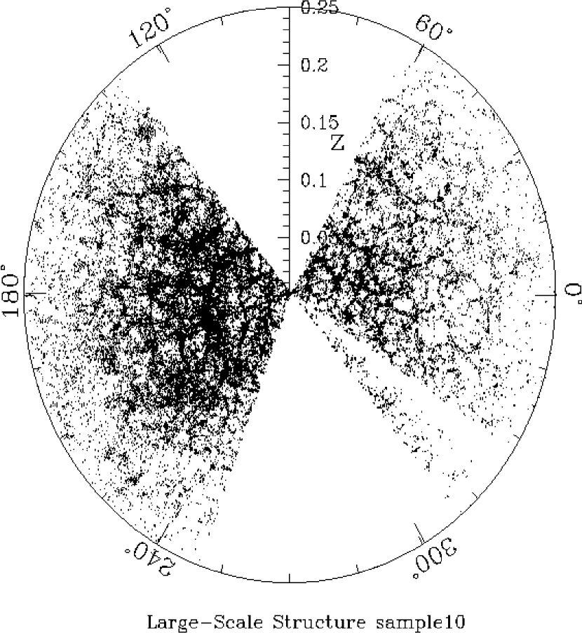
Figure 1: Equatorial distribution of right ascension and redshift for Main Sample galaxies within 6^∘ of the Equator in sample10 of the SDSS. The half of the survey in the Galactic South (on the right) appears less dense than the Galactic North (on the left) simply because the imaging near the equator extends less in the declination direction in the south than in the north.

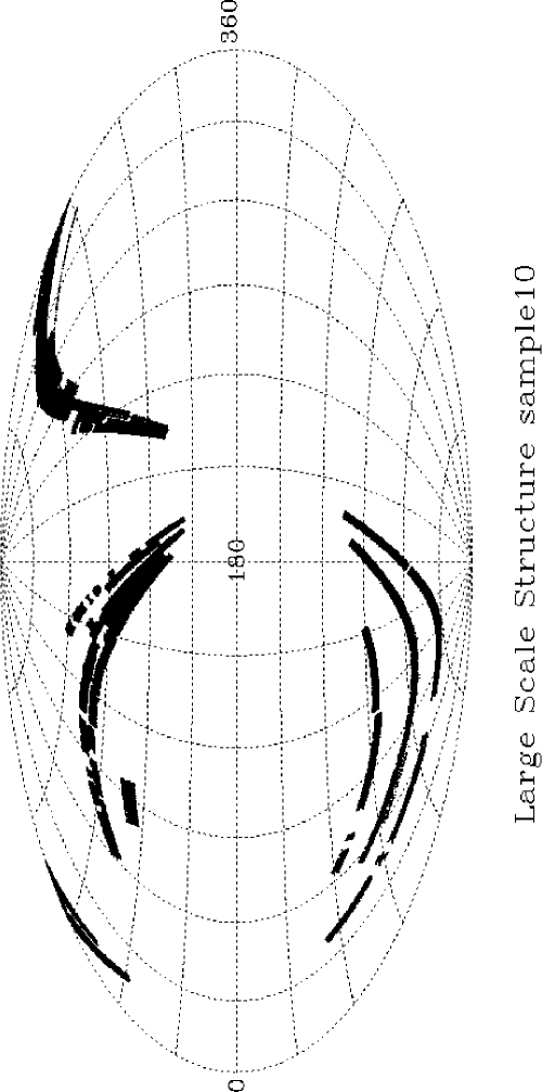
Figure 2: Distribution in Galactic coordinates of spectroscopically confirmed galaxies in the SDSS Large-Scale Structure sample10. The effective area covered (the integral of the SDSS sampling fraction over the covered area) is about 1844 deg².

As of April 2002, the SDSS had imaged and targeted 2,873 deg² of sky and taken spectra of approximately 350,000 objects over $\sim 2,000$ deg² of that area. From these results, we created a well-defined sample for calculating large-scale structure and galaxy property statistics, known as Large-Scale Structure sample10. sample10 consists of all of the photometry for all of the targets over that area (as extracted from the internal SDSS operational database), all of the spectroscopic results (as output from specBS), and, most significantly, a description of the angular window function of the survey and the flux and surface brightness limits used for galaxies in each area of the sky. For most of the area, the same version of the image analysis software used to create the spectroscopic target list was used in this sample. However, for the area covered by the Early Data Release (EDR; Stoughton et al. 2002) we used the version of the analysis software used for that data release, since it was substantially better than the early versions of the software used to target that area. For photo, the most important piece of analysis software run on the data, the versions used for the photometry range from v5_0 to v5_2. The region covered by this sample is similar to, but not exactly, the region which will be released in the SDSS Data Release 1 (DR1), scheduled for January 2003 (which will use photo v5_3, a newer version of the software which among other things improves the handling of large galaxies). Figure 1 shows the distribution in right ascension and redshift of Main Sample galaxies with redshifts in sample10 within 6^∘ of the Equator. Figure 2 shows the distribution of Main Sample galaxies with redshifts on the sky in Galactic coordinates.

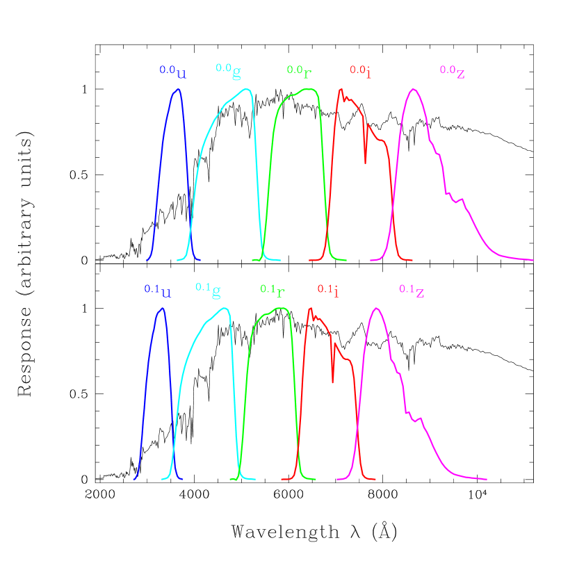
Figure 3: Demonstration of the differences between the unshifted SDSS filter system (${}^{0.0}\!{u}$, ${}^{0.0}\!{g}$, ${}^{0.0}\!{r}$, ${}^{0.0}\!{i}$, ${}^{0.0}\!{z}$) in the top panel and the SDSS filter system shifted by $0.1$ (${}^{0.1}\!{u}$, ${}^{0.1}\!{g}$, ${}^{0.1}\!{r}$, ${}^{0.1}\!{i}$, ${}^{0.1}\!{z}$) in the bottom panel. Shown for comparison is a 4 Gyr-old instantaneous burst population from an update of the Bruzual A. & Charlot (1993) stellar population synthesis models. The $K$-corrections between the magnitudes of a galaxy in the unshifted SDSS system observed at redshift $z=0.1$ and the magnitudes of that galaxy in the $0.1$-shifted SDSS system observed at redshift $z=0$ are independent of the galaxy’s spectral energy distribution (and for AB magnitudes are equal to $-2.5\log_{10}(1+0.1)$ for all bands; Blanton et al. 2002a). This independence on spectral type makes the $0.1$-shifted system a more appropriate system in which to express SDSS results, for which the median redshift is near redshift $z=0.1$.

We measure galaxy magnitudes through a set of bandpasses which is obviously constant in the observer frame. This set of observer frame magnitudes corresponds to a different set of rest-frame magnitudes depending on the galaxy redshift. In order to compare galaxies observed at different redshifts, we convert all the magnitudes to a single fixed set of bandpasses. To perform this conversion, we use the method of Blanton et al. (2002a) (kcorrect v1_11). These routines fit a linear combination of four spectral templates to each set of five magnitudes, assigning coefficients $a_{0}$, $a_{1}$, $a_{2}$, and $a_{4}$. The coefficient $a_{0}$ to the first template is an estimate of the flux in the optical range ($3500\mathrm{\AA}<\lambda<7500\mathrm{\AA}$) in ergs s^-1 cm^-2; the fractional contribution of the other coefficients $a_{1}/a_{0}$, $a_{2}/a_{0}$, and $a_{3}/a_{0}$ characterize the spectral energy distribution of the galaxy. The most significant variation is along $a_{3}/a_{0}$. Taking the sum of the templates and projecting it onto filter responses, we can calculate the $K$-corrections from the observed bandpass to any rest-frame bandpass. In order to minimize the uncertainties in the $K$-correction, we choose a fixed set of bandpasses blueshifted by $z=0.1$ in order that they cover the same region of the rest-frame spectrum as do the observed bandpasses for a galaxy at $z=0.1$ (chosen because it is near the median redshift of the sample). The bottom panel Figure 3 shows this set of shifted bandpasses in the SDSS (${}^{0.1}\!{u}$, ${}^{0.1}\!{g}$, ${}^{0.1}\!{r}$, ${}^{0.1}\!{i}$, ${}^{0.1}\!{z}$)); the top panel shows the more commonly used unshifted restframe bandpasses, measurements of which are more poorly constrained by our set of data.

For this paper, rather than using the full freedom of all four templates, we instead use $K$-corrections from a restricted set of models. We fix $a_{1}/a_{0}=0$ and $a_{2}/a_{0}=0$ (near the mean of the galaxy distribution in coefficient space). In addition, after fitting for $a_{3}/a_{0}$ we restrict that ratio to be one of the twelve values. Figure 4 shows the $K$-corrections in each band as a function of redshift for each of these twelve values. The reason to restrict the $K$-correction this way is to make the likelihood evaluation more efficient, as described in Blanton et al. (2002c). We have tested the effect of this approximation on our fit for the luminosity function by taking a smaller set of values (six), finding no significant differences. Furthermore, if we consider the residuals of the restricted $K$-corrections in Figure 4 to the $K$-corrections found using all four templates, there is no trend with redshift and the standard deviations of the differences are 0.03 mags at most (for the $u$ band; the value is much less for the other bands).

From this sample, we create one subsample for each band, $u$, $g$, $r$, $i$, and $z$, of galaxies satisfying the apparent magnitude and redshift limits listed in Table 1. We chose the same apparent magnitude limits for the bands other than $r$ as Blanton et al. (2001) chose; that paper chose the limits by imposing the requirement that $<2\%$ of galaxies brighter than the flux limit in the given band are fainter than $r^{\ast}=17.6$. By defining a separate magnitude-limited sample in each band, we avoid biasing our results in one band due to the fact that the galaxies were selected in another band (for example, if we calculated the luminosity function in the $u$ band from a sample limited in the $r$ band, all of the faintest $u$ band galaxies would tend to be red galaxies). For each band we include essentially all observed absolute magnitudes in our samples. However, we of course do not have good constraints at all absolute magnitudes; for this reason, we consider our model applicable only to a smaller range of evolution-corrected absolute magnitudes, which we define from the tenth least luminous object to the most luminous object. These absolute magnitude limits are also listed in Table 1.

3 Fitting the Luminosity Function

In this section, we describe how to recover the number density of galaxies $\Phi(M,z)$ as a function of absolute magnitude $M$ and redshift $z$, which we will use to calculate the luminosity density at $z=0.1$. Each galaxy has a measured magnitude in each band $m$, an associated uncertainty $\Delta m$, and a redshift $z$. The absolute magnitude $M_{{}^{0.1}\!{r}}$ may be constructed from the apparent magnitude $m_{r}$ and redshift $z$ as follows

$$M_{\mathrm{{}^{0.1}\!{r}}}-5\log_{10}h=m_{r}-\mathrm{DM}(z,\Omega_{0},\Omega_{\Lambda},h=1)-K_{{}^{0.1}\!{r}r}(z),$$ (6)

where as written $\mathrm{DM}(z,\Omega_{0},\Omega_{\Lambda},h=1)$ is the distance modulus as determined from the redshift assuming a particular cosmology (for example, using the formulae compiled by Hogg 1999) and $h=1$. $K_{{}^{0.1}\!{r}r}(z)$ is the $K$-correction from the $r$ band of a galaxy at redshift $z$ to the ${}^{0.1}\!{r}$ band.

In order to fit the distribution of the absolute magnitudes and redshifts of galaxies, we use a maximum likelihood method which allows for a generic luminosity function shape (it does not assume a Schechter function or any other simple form), allows for simple luminosity and number evolution, and accounts for the estimated uncertainties in the galaxy fluxes. The method is described in detail by Blanton et al. (2002c), and we outline it briefly here. It is akin to the stepwise maximum likelihood (SWML) method of Efstathiou et al. (1988). However, it includes evolution in our model for the luminosity function, it accounts for the effects of flux uncertainties, and (for computational convenience) it uses Gaussian basis functions rather than top hat basis functions. In addition, rather than maximizing the likelihood of absolute magnitude given redshift, it maximizes the joint likelihood of absolute magnitude and redshift. This choice makes our estimates more sensitive to large-scale structure in the sample, and more sensitive to evolution.

Our model for the luminosity-redshift function is

$$\Phi(M,z)={\bar{n}}10^{0.4(z-z_{0})P}\sum_{k}\Phi_{k}\frac{1}{\sqrt{2\pi\sigma_{M}^{2}}}\exp\left[-\frac{1}{2}\frac{\left(M-M_{k}+(z-z_{0})Q\right)^{2}}{\sigma_{M}^{2}}\right],$$ (7)

where the $M_{k}$ are fixed to be equally spaced in absolute magnitude and represent the centers of Gaussians of width $\sigma_{M}$. $\Phi_{k}$ are adjustable parameters signifying the amplitudes of the Gaussians.

Following Lin et al. (1999), $Q$ represents the evolution in luminosity, in units of magnitude per unit redshift; $Q>0$ indicates that galaxies were more luminous in the past. $P$ quantifies the change in the number density with redshift; we choose this particular parametrization (again following Lin et al. 1999) such that $P$ represents the contribution of number density evolution to the evolution in the luminosity density in units of magnitudes. $P$ can be interpreted as either due to true evolution in the number density or due to very large scale structure. Given the size of our data set and its relative shallowness, we cannot distinguish between these possibilities; when necessary to, we will interpret $P$ only as large-scale structure. In any case, our main interest in this paper is the luminosity density at $z=0.1$, not its evolution, and the luminosity density is insensitive to reasonable values of $P$. $z_{0}$ is the zeropoint redshift, with respect to which we measure the evolution; for this sample, we choose $z_{0}=0.1$, the median redshift, since it is at that redshift that we can observe galaxies in the luminosity range around $M_{\ast}$, which contribute the most to the luminosity density.

In principle we can include large-scale structure in the radial direction, $\rho(z)$, explicitly in the model, with the constraint that it have a reasonable power spectrum (since the power in the density field is constrained mostly by modes which are not purely radial). However, we have decided not to do so here because it is not necessary for our goals.

As described in Blanton et al. (2002c), we fit model parameters by maximizing the likelihood of the model parameters given the data:

$$\prod_{i}p(Q,P,\ln\Phi_{k}|M_{i},z_{i})=\prod_{i}\frac{p(M_{i},z_{i}|Q,P,\ln\Phi_{k})p(Q,P,\ln\Phi_{k})}{p(M_{i},z_{i})}$$ (8)

We assume a uniform prior distribution of $\ln\Phi_{k}$, $Q$, and $P$ (thus guaranteeing that $\Phi_{k}$ is positive). Because $p(M_{i},z_{i})$ obviously does not depend on the model parameters, the problem reduces to minimizing

$$E=-2\sum_{i}\log p(M_{i},z_{i}|Q,P,\ln\Phi_{k}).$$ (9)

We construct the likelihood $p(M_{i},z_{i}|Q,P,\ln\Phi_{k})$ of each galaxy $i$ by convolving the luminosity function with a Gaussian of width $\Delta m$ (the estimated apparent magnitude uncertainty defined above) and constraining the galaxies to satisfy the flux limits of the survey:

$$p(M,z|Q,P,\ln\Phi_{k})=\left\{\begin{array}[]{cc}\Phi(M,z)\otimes G(\Delta m)&\mathrm{if~{}}m_{\mathrm{min}}<M+\mathrm{DM}(z)+K(z)-(z-z_{0})Q<m_{\mathrm{max}}\cr 0&\mathrm{otherwise}\end{array}\right.$$ (10)

The number of parameters required for this fit ($50$–$100$) is small enough that standard function minimizers can handle the task in a reasonable amount of time (one hour) on modern workstations (in our case, a 2 GHz Pentium IV machine), for a sample of $\sim 10^{5}$ objects. In the fit, we constrain the integral of $\Phi(M,z=0.1)$ to be unity over our range of absolute magnitude (as listed in Table 1 for each band).

The overall normalization ${\bar{n}}$ cannot be determined from this likelihood maximization procedure. We use the standard minimum variance estimator of Davis & Huchra (1982) to perform the normalization.

$${\bar{n}}=\frac{\sum_{j=1}^{N_{\mathrm{gals}}}w(z_{j})}{\int dV\phi(z)w(z)},$$ (11)

where the integral is over the volume covered by the survey between the minimum and maximum redshifts used for our estimate. The weight for each galaxy is

$$w(z)=\frac{f_{t}}{1+{\bar{n}}10^{0.4P(z-z_{0})}J_{3}\phi(z)},$$ (12)

and the selection function is

$$\phi(z)=\frac{{\int_{L_{\mathrm{min}}(z)}^{L_{\mathrm{max}}(z)}dL\,\Phi(L,z)}}{{\int_{L_{\mathrm{min}}}^{L_{\mathrm{max}}}dL\,\Phi(L,z)}},$$ (13)

where $f_{t}$ is the galaxy sampling rate determined at each position of sky as the fraction of targets in each sector that were successfully assigned a classification. The integral of the correlation function is:

$$J_{3}=\int_{0}^{\infty}dr\,r^{2}\xi(r)=10000~{}h^{-3}~{}\mathrm{Mpc}^{3}.$$ (14)

Clearly, because ${\bar{n}}$ appears in the weight $w(z)$, it must be determined iteratively, which we do using the simple estimator ${\bar{n}}=(1/V)\sum 1/\phi(z_{j})$ as an initial guess.

To determine the uncertainties in our fit, we use thirty jackknife resamplings of the data. In each sampling, we omit $1/30$ of the effective area of sky (meaning, the area weighted by the sampling rate $f_{t}$). Each omitted area is a nearly contiguous set of sectors. This jackknife resampling procedure thus includes, to the extent possible, the uncertainties due to large-scale structure and calibration errors across the survey. Effectively, it includes the effects of errors which are correlated with angular position on the largest scales. Taking the results of all thirty fits to the data, we calculate the covariance between all of our measured parameters using the standard formula

$${\left\langle{\Delta x_{i}\Delta x_{j}}\right\rangle}=\frac{N-1}{N}\sum_{i}(x_{i}-{\bar{x}}_{i})(x_{j}-{\bar{x}}_{j})$$ (15)

The uncertainty correlation matrix is then defined in the standard way: $r_{ij}={\langle{\Delta x_{i}\Delta x_{j}}\rangle}/({\langle{\Delta x_{i}^{2}}\rangle}{\langle{\Delta x_{j}^{2}}\rangle})^{1/2}$.

We are not interested in the uncertainty correlations between the amplitudes of each Gaussian, because obviously neighboring Gaussians will be highly covariant. For this paper, we will not even be interested in the covariances between overall amplitude at different luminosities of the luminosity function calculated from the sum of the Gaussians. However, we will list in tables the covariances between the luminosity density, the evolution parameters, and overall measures of the shape, such as $M_{\ast}$ and $\alpha$ for the best fit Schechter function of each luminosity function. It is also important to track the covariances among the luminosity densities in all of the bands; because large-scale structure is an important source of uncertainty, the luminosity densities are highly covariant, and ignoring this covariance would lead to overconfidence in any fit to the stellar density in galaxies based on this data (and underconfidence in our knowledge of the relative luminosity density in different bands).

Note that the true uncertainties in the luminosity density may be dominated by the uncertainties in the overall photometric calibration or by the fraction of flux contained within the Petrosian aperture for the galaxies that contribute to the luminosity density, while the uncertainties in the level of evolution recovered may be dominated by possible systematic errors in the $K$-corrections, as well as a systematic dependence of the fraction of light contained within a Petrosian magnitude as a function of redshift (due to the effects of seeing).

4 Results

We have applied the procedure described in the Section 3 to the data described in Section 2. Our results are summarized in this section.

4.1 Luminosity Functions

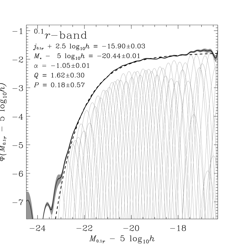
Figure 5: Luminosity function in the ${}^{0.1}\!{r}$ band. The thick solid line is the luminosity function fit; the thin solid lines are the individual gaussians of which it is composed. The grey region around the luminosity function fit represents the 1$\sigma$ uncertainties around the line; naturally, these uncertainties are highly correlated with each other. The dashed line is the Schechter function fit to the result. The luminosity density, the evolution parameters, and the parameters of the Schechter function are listed in the figure.

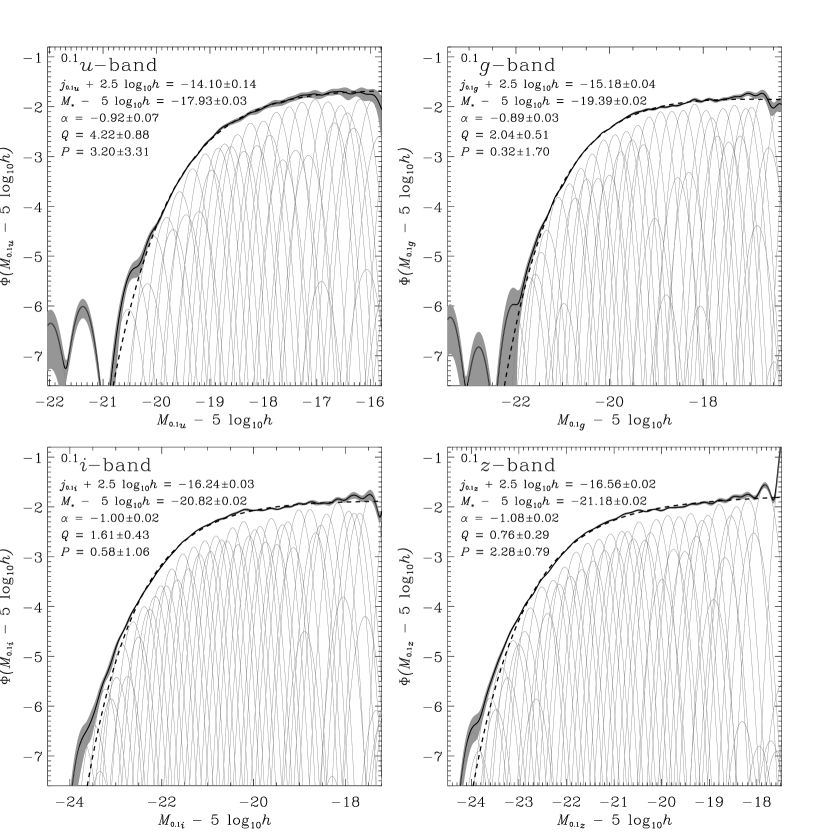
Figure 6: Same as Figure 5, for the ${}^{0.1}\!{u}$, ${}^{0.1}\!{g}$, ${}^{0.1}\!{i}$, and ${}^{0.1}\!{z}$ bands.

Figures 5 and 6 show the galaxy luminosity function in the ${}^{0.1}\!{u}$, ${}^{0.1}\!{g}$, ${}^{0.1}\!{r}$, ${}^{0.1}\!{i}$, and ${}^{0.1}\!{z}$ bands, assuming $\Omega_{0}=0.3$ and $\Omega_{\Lambda}=0.7$. The thick black line shows our best fit luminosity function. The thin black lines show the Gaussians which sum to form the full luminosity function. The grey region surrounding the thick black line indicates the 1$\sigma$ uncertainties in the luminosity function — of course, these uncertainties are all correlated with one another, and are closer to representing the uncertainties in the overall normalization of the function than the individual uncertainties at each magnitude. The best-fit $Q$ and $P$ evolution parameters are listed in the figure.

We have taken the thick black lines and their uncertainties and fit a Schechter function to each curve. The dotted lines in Figures 5 and 6 represent the best fit Schechter functions, which provide a reasonable fit to our non-parametric results. The luminosity density we list in the figure, expressed as the absolute magnitude from galaxies in an $h^{-3}$ Mpc³ on average, is the result of integrating this Schechter function fit over all luminosities. The values associated with the Schechter function are listed in Table 2. We list results for the ($\Omega_{0}=1.0$, $\Omega_{\Lambda}=0.0$) and ($\Omega_{0}=0.3$, $\Omega_{\Lambda}=0.0$) cosmologies as well. We have found that to an accuracy of about 3%, we can convert the results of one cosmology to those of another by scaling $\phi_{\ast}$ by the inverse ratio of the comoving volumes at $z=0.1$ between the two cosmologies, and by scaling $M_{\ast}$ by the difference of the distance moduli at $z=0.1$ for the two cosmologies. We therefore recommend this procedure for readers interested in comparing our results to those in some other cosmological model.

Table 3 lists some salient quantitative measurements of the luminosity function in each band, including the evolution parameters and the luminosity density (expressed in magnitudes, solar luminosities, and flux at the effective filter wavelength) for a Mpc³. To obtain the physical expressions of the luminosity density, we used measurements of the SDSS camera response performed by Mamoru Doi, which James Gunn combined with estimates of the atmospheric extinction as a function of wavelength at $1.3$ airmasses (to which all SDSS observations are calibrated) and the primary and secondary mirror reflectivities. Projecting the solar model of Kurucz (1991) onto these bandpasses (shifted to $z=0.1$) yields the absolute solar AB magnitudes:

$$M_{\odot,^{0.1}\!{u}}=6.80\mathrm{;}\quad M_{\odot,^{0.1}\!{g}}=5.45\mathrm{;}\quad M_{\odot,^{0.1}\!{r}}=4.76\mathrm{;}\quad M_{\odot,^{0.1}\!{i}}=4.58\mathrm{;}\quad M_{\odot,^{0.1}\!{z}}=4.51$$ (16)

The luminosity densities expressed in ergs s^-1 Å^-1 are calculated from the AB magnitudes as follows. First, we use the equation which relates an AB magnitude to the effective flux density at the effective wavelength,

$$f_{\lambda}=(3.631\times 10^{-20}\mathrm{ergs~{}cm}^{-2}\mathrm{~{}s}^{-1}\mathrm{~{}Hz}^{-1})\frac{c}{\lambda_{\mathrm{eff}}^{2}}10^{-0.4m},$$ (17)

to convert the absolute magnitudes in an $h^{-3}$ Mpc³ to the flux density which would be observed if an average $h^{-3}$ Mpc³ of the universe were compressed to a point source and placed 10 pc distant from the observer. Second, we multiply this value by $4\pi(10\mathrm{~{}pc})^{2}$ to obtain the average luminosity per unit wavelength at the effective wavelength in an $h^{-3}$ Mpc³. The “effective wavelength” of a passband with a quantum efficiency $R(\lambda)$ is defined:

$$\lambda_{\mathrm{eff}}=\exp\left[\frac{\int d(\ln\lambda)R(\lambda)\ln\lambda}{\int d(\ln\lambda)R(\lambda)}\right],$$ (18)

following Fukugita et al. (1996) and Schneider et al. (1983). The effective flux density defined above is that which an AB standard source ($f_{\lambda}(\lambda)\propto\lambda^{-2}$) of magnitude $m$ in passband $R$ would have at the effective wavelength. Both of these quantities are obviously only nominal since, in any case, the average spectrum of galaxies is nothing like an AB standard source, but it does give a sense of the physical flux associated with a magnitude. We also list $f_{\mathrm{np}}$, the fraction of the integrated luminosity density of the Schechter luminosity function included in the non-parametric estimate of the luminosity density. Results for the cosmologies ($\Omega_{m}=0.3$, $\Omega_{\Lambda}=0.0$) and ($\Omega_{m}=1.0$, $\Omega_{\Lambda}=0.0$) are also listed.

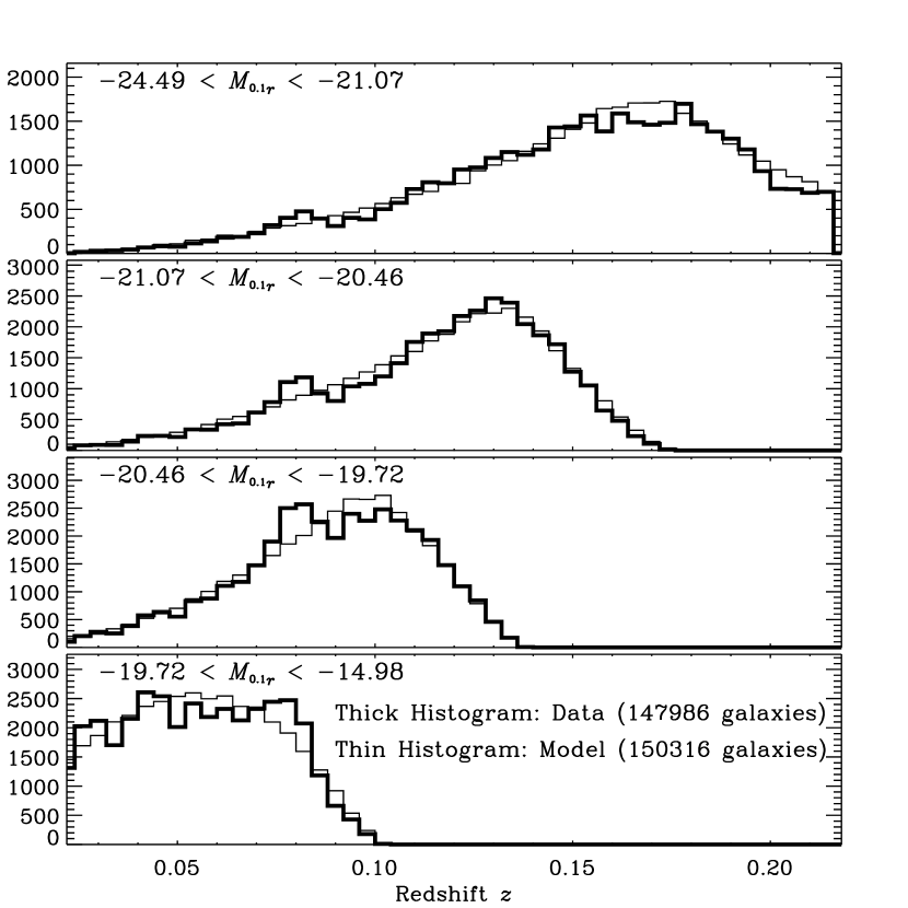
Figure 7: Redshift distribution of the ${}^{0.1}\!{r}$ band sample, for each quartile (weighted by number) in absolute magnitude. The thick line represents the data; the thin line is a Monte Carlo representation of the model, including the selection effects in the survey. In this figure and in the following Figures 8–12, the model is a decent representation of the data, but not a perfect one; much of the difference is likely to be due to large-scale structure, but it is possible that further complications of our evolution model or our error model might be necessary to fully reproduce the data.

It is worth asking how well this model reproduces the number counts of galaxies as a function of redshift and absolute magnitude. Figure 7 shows the redshift distribution of galaxies in our sample for quartiles in absolute magnitude in the ${}^{0.1}\!{r}$ band as a thick histogram. The expectation from our model fit (based on Monte Carlo realizations of the sample) is shown as the thin histogram. Figures 8–12 show the counts in bins of absolute magnitude for several slices in redshift. Again, the thick histogram represents the data and the thin histogram represents the model. The model appears to the eye to be a reasonable fit to the data. However, it is clear that there are statistically significant discrepancies in these figures (note the large number of objects in each bin). Some of these discrepancies occur because there is large-scale structure in the sample; however, it is possible that we will need to introduce a more sophisticated model for the evolution of the galaxies or for the relationship between density and luminosity in order to explain all of these discrepancies. As discussed in the conclusions, we postpone the investigation of these issues to a later paper.

As described above, we have quantified our uncertainties by taking 30 jacknife resamplings of the data. In Tables 4–8 we display the resulting correlation matrices between various properties of our fit for each band. Note that many of the parameters are highly correlated. In particular we note that $M_{\ast}$ and $\alpha$, which characterize the shape of the Schechter luminosity function, are highly correlated. One should be cautious when quoting $M_{\ast}$ values as representative of the “typical luminosity” of a luminous galaxy. This statement is true to an extent, but not in detail.

Table 9 displays the correlation matrix between the luminosity densities and evolution parameters $Q$ in all of the bands. Note that this matrix is entirely positive. In any particular resampling, if the luminosity density is slightly high in one band relative to the mean, all the bands are slightly high; when one band evolves a bit more strongly, so do they all. This correlation occurs because our errors are dominated by large-scale structure, which affects all the bands simultaneously. These correlations are strong, so it is important to account for this correlation matrix of uncertainties when using these results.

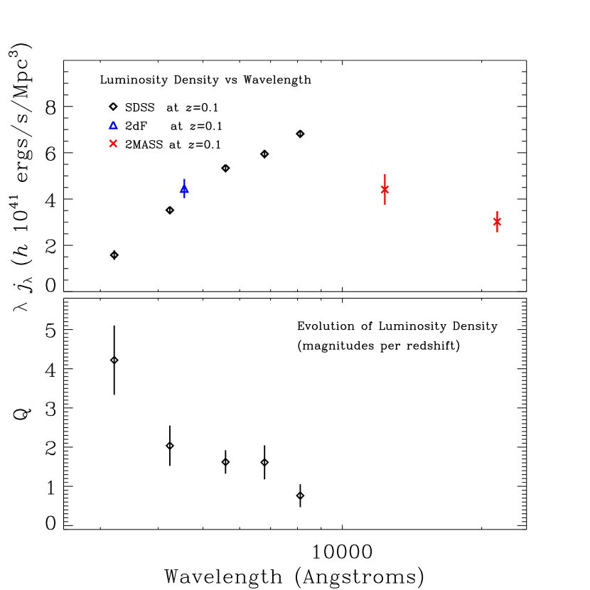
Figure 14: Luminosity density and its evolution as a function of wavelength, for the SDSS (diamonds; this paper), the 2dFGRS (triangle; Norberg et al. 2002), and 2MASS (crosses, Cole et al. 2001). The 2dFGRS has been evolution-corrected to $z=0.1$ using $Q_{b_{j}}=1$ (the effective value used by Norberg et al. 2002) and 2MASS has been evolution-corrected to $z=0.1$ using $Q_{J}=Q_{K}=1$.

The top panel of Figure 14 shows the luminosity density as a function of wavelength at $z=0.1$ using the results of all five bands.

4.2 Galaxy Luminosity Density Evolution

One product of our fit is $Q$, the evolution of the luminosity density. However, we caution that we have restricted our model such that galaxies of all luminosities evolve identically. This assumption is probably incorrect, because different galaxy types have different luminosity function and are expected to evolve in different ways (since their differing colors obviously imply different star-formation histories). Furthermore, our understanding of our photometric error model, particularly in $u$ and $z$, is currently rather primitive. While we believe that the flaws in our model for the evolution do not greatly bias the main result of this paper, the luminosity function and luminosity density at $z=0.1$, we do warn the reader that because of the deficiencies of our model the measured $Q$ values might be biased.

We show our results for the luminosity evolution, $Q$, and its uncertainties, in the bottom panel of Figure 14, for all the bands. The ${}^{0.1}\!{u}$ band has very strong evolution ($Q\sim 4$), although with large uncertainties. The other bands all have $Q\sim 1$–$2$. The evolution in these bands is generally consistent with the evolution of a relatively old stellar population. However, we will consider fits to theoretical models more carefully in a separate paper, and draw no particular conclusions here.

It is likely that these evolution results reflect the evolution of the more luminous galaxies in the sample, for two reasons. First, more luminous galaxies are observable over a larger redshift range. Second, the low luminosity end of the luminosity function is nearly a power-law, which makes it more difficult to detect evolution. If $Q$ traces the evolution of primarily the luminous galaxies, it might explain why the evolution in the ${}^{0.1}\!{u}$ band is unusually large; the most luminous objects in the ${}^{0.1}\!{u}$ band are the blue, exponential profile objects, which we expect to evolve more rapidly than red, concentrated galaxies.

For the flat, $\Lambda$-dominated cosmology, ${}^{0.1}\!{u}$ and ${}^{0.1}\!{z}$ bands have $P\neq 0$, though at low significance in the case of ${}^{0.1}\!{u}$. We do not believe that $P$ reflects true number density evolution, which we regard as a priori unlikely, especially since the other bands have $P$ consistent with zero. Instead $P$ probably is compensating for inaccuracies in some other aspect of our model. In the case of the ${}^{0.1}\!{u}$ band it may compensate for the fact that our model does not include large-scale structure. In the case of the ${}^{0.1}\!{z}$ band, our error model could be insufficient, or the $K$-corrections might be incorrect (though they are small in any case). Thus, one might claim that the luminosity density evolution we measure should be $Q+P$; however, we think it better to interpret a non-zero $P$ to reflect large-scale structure in the sample rather than true evolution. A more sophisticated approach would be to treat the problem in more detail by fitting for the radial large-scale structure simultaneously with the luminosity function.

We note in passing that the differences in $P$ and $Q$ between the flat, $\Lambda$-dominated cosmology and the other cosmologies are consistent with the differences in the redshift dependence of the luminosity distance and the differential comoving volume among these cosmologies. We do not regard the low value of $P$ for $g$, $r$, and $i$ in the flat, $\Lambda$-dominated cosmology necessarily as evidence that that cosmological model is correct.

5 Systematics Tests of Petrosian Magnitudes

One of the challenges in studying the luminosity function and its redshift dependence is that one must verify that one’s measurements of galaxy luminosity are consistent as a function of redshift. That is, one must test whether observing an identical galaxy at different redshifts will yield the same fraction of the total independent of redshift. Otherwise, systematic errors in the measurement of galaxy luminosities as a function of redshift could masquerade as evolution.

Several :w effects can yield artificial redshift dependence in one’s determination of galaxy flux (which is to say, redshift dependence which cannot be accounted for using the distance modulus and the $K$-correction). First, the increased physical size corresponding to the angular PSF width for galaxies at high redshift can change both the metric size (in physical units at the galaxy) of the aperture used to calculate the galaxy flux and the amount of light scattered outside of any particular aperture. Second, color gradients in galaxies mean that the different radii in the galaxy profile $K$-correct differently. Since in the SDSS the size of the aperture is based on the shape of the profile, this effect can change the metric size of the aperture used to calculate the galaxy flux. Third, cosmological surface brightness dimming can make the outermost measurable isophote have a smaller metric size.

Because the SDSS has high signal-to-noise ratio imaging and because it uses Petrosian rather than isophotal magnitudes, the third effect is negligible. However, Petrosian magnitudes are sensitive to some degree to seeing; as an object becomes small with respect to the seeing width, the fraction of the total flux measured by the Petrosian magnitudes tends to that fraction for a pure PSF (e.g. Blanton et al. 2001, Strauss et al. 2002). For the SDSS, the fraction of the total light in a pure PSF measured by the Petrosian magnitude is about 95%. Thus, galaxies with exponential profiles will tend to have their measured fluxes reduced in the presence of bad seeing from the fraction of nearly 100% for the no-seeing case. On the other hand, galaxies with de Vaucouleurs profiles will tend to have their measured fluxes increased from the fraction of only 82% for the no seeing case. Furthermore, the apertures of the Petrosian magnitudes are determined by the $r$-band image of the galaxy, which, while it is less sensitive to differential $K$-corrections than bluer bands, is still somewhat dependent on these effects.

Several methods exist for estimating what fraction of the flux is outside the SDSS Petrosian apertures. First, one could compare SDSS imaging to deeper imaging. Second, one could stack many SDSS images of different galaxies but of similar types, and use the composite profile to characterize the fraction of light missing outside of a Petrosian aperture. Third, one can use a reasonable model for galaxy light profiles to extrapolate to a “total” flux for each object. Here, we take the third approach, using the Sérsic magnitudes described in Section 2 as a seeing-corrected, “total” magnitude. In addition, because the Sérsic fit is based on the $i$-band image, the issue of the $K$-correction of the galaxy profile is negligible (as the $K$-corrections in the $i$-band are small) for the redshifts considered in this paper.

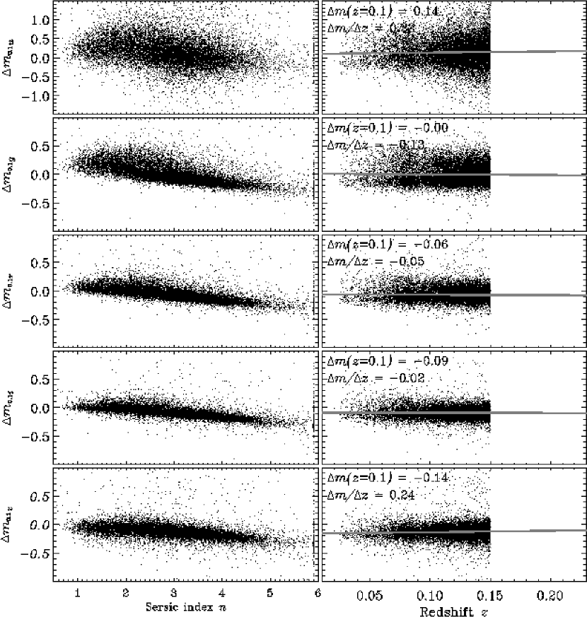
Figure 13: Differences $\Delta m\equiv m_{S}-m_{P}$ between Sersic and Petrosian magnitudes for each band for a volume-limited sample with $-23<M_{{}^{0.1}\!{r}}<-21$ and $0.02<z<0.15$. The left column shows the differences as a function of Sersic index $n$. As expected, for galaxies at high Sersic index (close to the de Vaucouleurs value $n=4$) the Petrosian magnitudes are an underestimate relative to Sersic magnitudes. For $r$, $i$, and $z$, the differences between the two remain small at low Sersic index (near the exponential value $n=1$). The right column shows the differences as a function of redshift $z$. A linear regression is shown as a grey line, along with the parameters associated with the best-fit regression. The slopes are generally insignificant compared to our uncertainties in the evolution parameter $Q$.

Figure 13 shows the differences between Sérsic and Petrosian magnitudes in each band, as a function of Sérsic index $n$ and redshift $z$. Clearly, the difference is sensitive to the Sérsic index and is larger for galaxies which are similar to de Vaucouleurs galaxies, in accordance with the estimates in Blanton et al. (2001) of the fraction of flux included in the SDSS Petrosian magnitudes for different profile types. For $u$ and $g$ the Sérsic magnitude is significantly fainter than the Petrosian magnitude at low Sérsic index. This fact might reflect color gradients within exponential galaxies. The shape of the Sérsic model we use is determined in the $i$-band; if the effective size of the galaxy is larger in bluer bands, known to be the case for spiral galaxies, the flux determined by fitting the Sérsic model amplitude will be smaller than the flux determined by counting the flux within an unweighted aperture. The right panel shows a linear regression versus redshift. The mean offset at $z=0.1$ ranges from 0.14 for the ${}^{0.1}\!{u}$ band to -0.14 for the ${}^{0.1}\!{z}$ band. Again, this result suggests that the Sérsic magnitude traces a redder population, perhaps as a consequence of color gradients in galaxies.

For our purposes here, we are interested primarily in the differences in the resulting luminosity density from Sérsic magnitudes relative to Petrosian magnitudes. When we fit luminosity functions to all five bands using the Sérsic magnitudes, we obtain luminosity densities offset from the Petrosian values as follows:

$$j_{{}^{0.1}\!{u}}(\mathrm{Sersic}) = j_{{}^{0.1}\!{u}}(\mathrm{Petrosian})-0.01$$ (19)

$$j_{{}^{0.1}\!{g}}(\mathrm{Sersic}) = j_{{}^{0.1}\!{g}}(\mathrm{Petrosian})-0.03$$ (20)

$$j_{{}^{0.1}\!{r}}(\mathrm{Sersic}) = j_{{}^{0.1}\!{r}}(\mathrm{Petrosian})-0.03$$ (21)

$$j_{{}^{0.1}\!{i}}(\mathrm{Sersic}) = j_{{}^{0.1}\!{i}}(\mathrm{Petrosian})-0.06$$ (22)

$$j_{{}^{0.1}\!{z}}(\mathrm{Sersic}) = j_{{}^{0.1}\!{z}}(\mathrm{Petrosian})-0.10$$ (23)

The values of $Q$ for Sérsic magnitudes are consistent with the results for Petrosian magnitudes. We caution that the estimates of the luminosity density using Sérsic magnitudes are not necessarily more correct than the estimates from Petrosian magnitudes; because the Sérsic profile is not a perfect fit to the observed radial profiles of galaxies, there is likely to be a bias in the resulting estimates of luminosity density associated with Sérsic magnitudes. However, the small differences in Equation (19) suggest that the differences are also small between either of these estimates and the luminosity density we would derive using true “total” magnitudes.

6 Comparison with Other Results

6.1 Galaxy Luminosity Density in Other Bands

In order to compare our results to those of other investigators, we have used the routines in kcorrect v1_14 (a slight update on the version kcorrect v1_11 used elsewhere in this paper and in Blanton et al. 2002a) to fit the SED of the universe and derive the luminosity densities in other bands. In particular, we list in Table 10 results for the unshifted SDSS bandpasses for comparison to Blanton et al. (2001), for the unshifted $B$, $V$, $R$ and $I$ Johnson bandpasses (using the responses listed by Bessell 1990), and for $b_{j}$ for comparison to 2dFGRS. To create the $b_{j}$ result we applied the equation $b_{j}-B=-0.28(B-V)$ to the results in the Johnson bandpasses, originally from Blair & Gilmore (1982). We derive these luminosity densities both at $z=0.1$ and (by using $Q$ to evolve the SDSS results) $z=0$. For comparison, we show in the same table the results of Blanton et al. (2001) and Norberg et al. (2002). For the Norberg et al. (2002) we use the mean evolutionary correction from their Figure 8 to evaluate a luminosity density at $z=0.1$. There is only 0.09 magnitude difference between our result in $b_{j}$ at $z=0.1$ and theirs; this difference is less than 1$\sigma$ taking into account the 2dFGRS statistical uncertainties.

The results of Table 10 reflect a general agreement between these different determinations of the luminosity function. In contrast to these results, Blanton et al. (2001) reported a higher luminosity density than found in other surveys, such as the 2dFGRS results of Folkes et al. (1999) and the Las Campanas Redshift Survey (LCRS; Shectman et al. 1996) results of Lin et al. (1996). Most recently, Liske et al. (2002) found that the ${}^{0.0}\!{g}$-band luminosity function of Blanton et al. (2001) overpredicted the number counts of galaxies found in the Millenium Galaxy Catalog. Furthermore, as pointed out by Wright (2001), the luminosity density in the ${}^{0.0}\!{z}$-band reported by Blanton et al. (2001) was unreasonably high relative to the luminosity density found by Cole et al. (2000) in ${}^{0.0}\!{J}$ and ${}^{0.0}\!{K}$. While our luminosity density is still considerably higher than that found by the LCRS, we no longer disagree significantly with 2dFGRS. Naturally, the question arises as to why the discrepancy existed in the first place.

Table 10 makes clear that there are large differences between our present results and those of Blanton et al. (2001). We should emphasize here that if we apply the same methods used in that paper to our current sample, the results are within 1$\sigma$ of the results in that paper. This change in the luminosity density estimates are not due to statistical fluctuations, nor to a change in the photometric calibration, but are instead due to improvements in our model for the luminosity function and the observations. In particular, we are using a better estimate of the $K$-corrections and we are including evolution in our model for the luminosity function. The largest changes are the luminosity densities in the ${}^{0.0}\!{u}$ and ${}^{0.0}\!{g}$ bands (which are 1.2 and 0.75 magnitudes less luminous respectively), where the changes in the $K$-corrections were largest and where evolution is most important. Ignoring evolution in the luminosity function model causes a large bias in the estimate of the luminosity density, because it causes the expected number of objects at high redshift to be inaccurate. If galaxies in fact are brighter in the past, a non-evolving model tends to yield lower number counts at high redshift, at a given normalization. Since the normalization procedure of Davis & Huchra (1982) weights according to volume, and thus accords higher weight at higher redshift, in this case a non-evolving model would result in an overestimate of galaxies at low redshift. Due to bad luck, the systematics comparison of Figure 8 in that paper, which compared the normalizations of the luminosity function at high and low redshift, happened not to reveal this effect, presumably due to the large supercluster at $z\sim 0.08$ in those data (and still distinctly visible in Figure 7 in this, much larger, dataset!). Figures 7–12 in the present paper show decisively that our current model explains the redshift counts very well.

So how does this affect our comparisons to other surveys? For the LCRS, whose method of fitting the luminosity function and its normalization was identical to that of Blanton et al. (2001), the original comparison remains the fair one. That is, even though our estimate of the luminosity density is now only $0.2$ magnitudes brighter than that of Lin et al. (1996), this is only an accident, resulting from a combination of two effects in the LCRS: using bright isophotal magnitudes, which lowers the luminosity density estimate, and ignoring (as Blanton et al. 2001 also did) evolution, which raises the luminosity density estimate. For 2MASS, the change in our result makes the SDSS more compatible with the results of Cole et al. (2001). However, it is more difficult to directly compare these surveys, since the SDSS bands and 2MASS bands do not overlap.

For the 2dFGRS, Norberg et al. (2002) report a luminosity density of $j_{b_{j}}=-15.35$ absolute magnitudes at $z=0$ (integrating the Schechter function for the $\Omega_{0}=0.3$, $\Omega_{\Lambda}=0.7$ cosmology in the first line of their Table 2 over all luminosities). This result is based on extrapolating to $z=0$ the luminosities of galaxies whose typical redshifts are $z=0.05$–$0.2$, using assumptions about the luminosity evolution. Figure 8 of Norberg et al. (2002), which shows the mean $K$-correction and evolution correction used in their analysis, shows that their evolution correction corresponds closely to $Q=1$. Since we find a somewhat different value of $Q\sim 2$ at these wavelengths, and both surveys have similar median redshifts, the fair comparison of the luminosity densities involves evaluating the luminosity density at around $z=0.1$. For this reason, we evolution-correct their results back to $z=0.1$ by applying $\Delta m=-0.1Q=-0.1$. Thus, for 2dFGRS $j_{b_{j}}(z=0.1)=-15.45\pm 0.1$, within 1$\sigma$ of our result in Table 10. Note that if we instead compare our $z=0$ value of the $b_{j}$ luminosity density to theirs, the discrepancy is about 0.2 magnitudes. However, in either comparison the differences between the SDSS and 2dFGRS luminosity densities are rather small.

We find similarly small differences between our results and the galaxy counts data from the Millenium Galaxy Catalog of Liske et al. (2002). Our Schechter function model for the ${}^{0.1}\!{g}$-band luminosity function, crudely transformed into $B_{\mathrm{MGC}}$ bandpass by applying $-0.09$ to $M_{\ast}$, and using $Q=2$ as for ${}^{0.1}\!{g}$, nicely predicts their galaxy counts to $B_{\mathrm{MGC}}=20$ to within about 5%.

The original Folkes et al. (1999) 2dFGRS result that Blanton et al. (2001) compared to did not evolution-correct their magnitudes either. So why was there a discrepancy between those two results? First of all, as Norberg et al. (2002) have pointed out, the linear transformation used by Blanton et al. (2001) to convert SDSS magnitudes to 2dFGRS magnitudes (which was based on the linear transformation between $b_{j}$ and $B$ and $V$ published by Metcalfe et al. 1995) was inappropriate. Using the Blair & Gilmore (1982) transformation from $B$ and $V$ to $b_{j}$ ($b_{j}-B=-0.28(B-V)$) instead results in a 10% reduction in the luminosity density, not enough to explain the original discrepancy. However, one significant difference between Folkes et al. (1999) and the mock $b_{j}$ luminosity function in Blanton et al. (2001) was that Folkes et al. (1999) normalized to the number counts instead of using a volume-weighted method. Due to this normalization, the Folkes et al. (1999) result was less affected by luminosity evolution, because their normalization was set by galaxies close to the median redshift of the survey, rather than those at the distant edge of the survey. This difference seems to account for the bulk of the discrepancy between Blanton et al. (2001) and Folkes et al. (1999). Norberg et al. (2002) reach the same conclusion. As stated above, comparison of our results to those of Norberg et al. (2002), who perform an evolution correction to their magnitudes, now results in a consistent measurement of the luminosity density.

Nevertheless, Blanton et al. (2001) did show that the isophotal magnitudes meaured by the APM survey did not include a significant fraction of the flux for a typical galaxy, and further that the “Gaussian-correction” to total magnitudes (described in detail by Maddox et al. 1990) performed on the galaxy fluxes were insufficient to replace this difference. If this were the whole story, there should remain a difference of roughly 30% between the Norberg et al. (2002) results based on 2dFGRS magnitudes and the results presented here, based on SDSS Petrosian magnitudes. However, extensive further calibration of the plate magnitudes has been performed using deep CCD imaging, as described by Norberg et al. (2002). In effect, the overall calibration of the galaxy survey is set by a comparison between observations of a set of galaxies using the APM and using deep CCD imaging. Since the magnitudes in the deep CCD imaging count flux outside the limiting isophotes of the APM magnitudes, this overall calibration translates the isophotal to total magnitudes (on average, that is — naturally, for any particular galaxy the correction depends on the profile shape and size of that galaxy). For this reason, the comparisons in Norberg et al. (2002) of 2dFGRS magnitudes and SDSS magnitudes agree on average, for galaxies near the median surface brightness (although there is a strong correlation of the residuals with surface brightness). Blanton et al. (2001) did not account for these extra step of calibration and isophotal-to-total correction, and so overestimated the effect of the different magnitude definitions in the final luminosity density.

Both Liske et al. (2002) and Cole et al. (2001) have suggested that the results of Blanton et al. (2001) could have been biased high due to large-scale structure. This possibility can be ruled out by simply using the same methods used by that paper on the full sample presented here. The luminosity density so calculated is within $1\sigma$ of the original result, suggesting that the 10% uncertainties calculated for that sample were realistic. This agreement occurs despite the fact that the galaxy counts for $r<17.7$ in the region used by Blanton et al. (2001) are 10–15% higher than in the survey on average. As correctly pointed out by Norberg et al. (2002), the statistical uncertainties in the normalization are much smaller when using the volume-weighting method of Davis & Huchra (1982), rather than the normalizing to galaxy counts, though as those authors state one is more susceptible to systematic errors in the model for evolution. Using the luminosity function model in this paper, normalizing either way yields nearly identical results; for example, consider the counts predicted by the models listed in Figures 8–12. The possible exception is the $u$-band, for which there is a 10% difference (still within the $1\sigma$ statistical uncertainties). Again, we emphasize that the differences between the luminosity function derived here and in Blanton et al. (2001) are a product primarily of the model of the luminosity function we use.

In short, the discrepancies between SDSS and 2dFGRS appear to be resolved, for the most part due to a proper treatment of evolution in the SDSS luminosity function. It remains to be determined whether the results of SDSS and 2MASS are discrepant, but in any case they are ameliorated by the reduction of our estimate of the luminosity density.

6.2 Luminosity Density as a Function of Wavelength

Figure 14 plots the luminosity density versus wavelength using Equation (17) for the SDSS (diamonds). Using the above results, we add the 2dFGRS point from Norberg et al. (2002) (triangle), and the 2MASS points from Cole et al. (2001) (crosses), as described in this section.

For the 2dFGRS, translating the luminosity density expressed in magnitudes into physical units is a nontrivial endeavour. The zeropoint of the 2dFGRS $b_{j}$ system is set by the equation:

$$b_{j}-B=-0.28(B-V).$$ (24)

Although this slope was determined by Blair & Gilmore (1982) based only on a small set of stars, it can be checked a posteriori against CCD observations which are appropriately converted from their natural system into the Johnson $B$ and $V$ system. According to Norberg et al. (2002), such observations confirm the slope $-0.28$ to a surprising degree of accuracy given the estimated errors of Blair & Gilmore (1982). However, the typical galaxy used to perform this check is not anywhere near $B-V=0$, and because we expect the relationship between any set of bandpasses to be nonlinear (with or without photographic plate nonlinearities), it is not guaranteed that $b_{j}$, as zeropointed using Equation (24, is a Vega-relative magnitude. We perform a test of Equation (24) using an estimate of the spectral response of the plates, from Hewett & Warren (private communication), who have determined the response for one plate by dispersing a spectrum (with well-measured $f_{\lambda}(\lambda)$ from spectrophotometry) through 2mm of GG395 filter and onto Kodak IIIaJ emulsion, the definition of the $b_{j}$ bandpass. Using the nominal $B$ and $V$ responses derived by Bessell (1990) and typical galaxy spectra at $z=0$, we find that the relationship between $b_{j}$ and $B$ around a typical galaxy color of $B-V\sim 0.8$ is close to $b_{j}-B\approx 0.04-0.28(B-V)$. The relationship is indeed nonlinear and appears to cross $b_{j}-B=0$ at $B-V=0$. Again, if this difference existed in the 2dFGRS data, it would never be noticed because the zeropoint is explicitly set using CCD imaging of galaxies assuming Equation (24) holds at typical galaxy colors. On the other hand, the curve given to us by Hewett & Warren is based only on measurements of a single plate, whose response may not be typical of the plates in the APM. Given this uncertainty, we simply assume Hewett & Warren are correct, and derive an AB magnitude from 2dFGRS $b_{j}$ magnitudes:

$$b_{j}(\mathrm{AB})=b_{j}(\mathrm{2dFGRS})+0.04-0.07,$$ (25)

which we claim is uncertain at the 0.05 mag level. Then we can use Equation (17) to calculate the luminosity density in physical units.

In the near infrared, the Two-Micron All Sky Survey (2MASS) results of Cole et al. (2000) for the ${}^{0.0}\!{J}$ and ${}^{0.0}\!{K_{s}}$ bands are shown. We use the published responses of $J$ and $K_{s}$ from the 2MASS website and the Kurucz (1991) theoretical Vega spectrum (normalized at 5000 Å to match the Hayes (1985) spectrophotometry of Vega) to calculate zeropoint shifts from Vega to AB magnitudes of ($0.91$, $1.85$) for $J$ and $K_{s}$, respectively. The $J$ band AB zeropoint corresponds closely with that listed in the 2MASS Explanatory Supplement Section IV.5.a. However, the $K_{s}$ band AB zeropoint listed there is about 1.77; since the spectrophotometry or model used to calculate this zeropoint is not specified on that site, we cannot determine the source of this discrepancy. However, the difference is within the 1$\sigma$ statistical uncertainties of Cole et al. (2001). To evolution-correct the 2MASS luminosity densities to $z=0.1$, we assume $Q=1$, which is consistent with most stellar population synthesis models. We display this in Figure 14 as crosses.

We should note here that although we have done our best here to place all the observations on the same physical footing, absolute calibration of this sort is uncertain. No spectrophotometry we know of has been performed to verify the models of Kurucz (1991) in the infrared, which we rely on to put the 2MASS results in physical units in Figure 14. There are uncertainties of at least 5% percent in the spectrophotometric calibration of BD+17 4708, the primary standard used to calibrate the SDSS. In any of the observations there is uncertainty and quite possibly variability in the bandpass responses. So this plot (and any plot like it in the literature) should not be trusted to better than 5% (which can be enough to substantially change one’s theoretical interpretation of the observations in terms of a star-formation history).

We leave until a later paper or to other authors a serious attempt to reconcile these various observations given a star-formation history and stellar population synthesis models.

7 Conclusions and Future Work

We have presented the galaxy luminosity density across the optical range, and have shown that it is consistent with other determinations. Previous differences found between the SDSS and other surveys are primarily attributable to the effect of luminosity evolution on our results. We have accounted for luminosity evolution in our current fits, and have given our results, which appear loosely consistent with the predictions of passive evolution in most bands. Our results are similar to those found by Bernardi et al. (2002) for their sample of early-type galaxies.

We note that our results are in general agreement with the shape of the cosmic spectrum determined from the 2dFGRS and SDSS galaxy spectra by Baldry et al. (2002) and Glazebrook et al., in preparation. In the case of SDSS spectra, Glazebrook et al. use the same data as used here (Petrosian magnitudes in sample10) to apply an overall normalization to their spectrum, but use the $3^{\prime\prime}$ diameter fiber spectra (which typically contain about 20% of the Petrosian galaxy flux and cover regions of the galaxy about 0.1 mag redder in $g-r$ than that covered by the Petrosian aperture) to find the luminosity density as a function of wavelength. The power of their approach is that the emission and absorption lines contain more detailed information on the star-formation history than do broad-band colors; the question remains whether this star-formation history is representative of the global star-formation history.

We will continue to improve our estimates of evolution. First, we will quantify our uncertainties in flux measurements more robustly and understand how our estimates of magnitude are affected by seeing in more detail. Doing so will yield more reliable estimates of luminosity evolution. Second, different galaxy types are expected to evolve differently; redder galaxies are generally presumed to be older and thus more slowly evolving. The different evolution of different galaxy types can constrain theories of the formation of galaxies, and thus it is of interest to study this differential evolution. Furthermore, it is well known that different galaxy types have different luminosity functions (e.g., Blanton et al. 2001); thus, it is probable that the shape of the galaxy luminosity function evolves, not merely its overall luminosity scale.

One caveat to our results is the existence of surface-brightness selection effects. Blanton et al. (2001) demonstrated that if the SDSS can truly detect most of the objects which exist down to $\mu_{r,50}\sim 24$, not much luminosity density ($\sim 5\%$) can exist at lower surface brightnesses, unless the dependence of luminosity on surface brightness flattens dramatically below these limits or there is a sharp upturn in the luminosity function at low luminosities. Cross et al. (2001) demonstrated similar results for 2dFGRS. This result is not necessarily inconsistent with the results of O’Neil & Bothun (2000), who found that the number density of galaxies does not decline at low surface brightnesses; however, if the relationship between luminosity and surface brightness measured in the SDSS exists in their galaxy sample, the contribution to the luminosity density of galaxies should decline considerably at low surface brightness. Unfortunately, that paper and its predecessors do not evaluate the luminosity density contributed by different ranges of surface brightness in their sample.

The possibility remains that the SDSS is very incomplete at $\mu_{r,50}\sim 24$. Such incompleteness would probably not be due to low signal-to-noise (see the order-of-magnitude calculation in Blanton et al. 2001); it would more likely be due to systematic difficulties in subtracting the sky background. We find no evidence for changes in the measured extinction-corrected surface-brightness distribution at Galactic extinctions varying from 0 to nearly 2 in the $r$-band (as determined by Schlegel et al. 1998), which indicates that the surface brightnesses of most galaxies in the survey are not close to the surface brightness limit of the survey. In fact, there are a number of “objects” detected at low surface brightness $\mu_{r,50}>24$, nearly all of which turn out to be scattered light or other image defects; thus, such low surface brightness features are readily detectable. We can test these effects more thoroughly by searching for simulated galaxies inserted into actual data, and such tests are currently ongoing.

These results (and the accompanying covariance matrices) can be used to constrain aspects of the star-formation history of the universe, and in particular the overall stellar density. In addition, they can be used to develop a selection function for flux-limited galaxy redshift surveys selected from the SDSS. They also provide the state-of-the-art luminosity densities with which to calculate $\Omega_{m}$ using measured mass-to-light ratios. Finally, they can be compared to high redshift estimates of luminosity density in order to evaluate the evolution of galaxies to high redshift.

Table 1: Selection limits

Band	Flux Limit	Redshift Limits	Absolute Magnitude Limits	Number of Galaxies
${}^{0.1}\!{u}$	$m_{u}<18.36$	$0.02<z<0.14$	$-21.93<M_{{}^{0.1}\!{u}}-5\log_{10}h<-15.54$	$22020$
${}^{0.1}\!{g}$	$m_{g}<17.69$	$0.02<z<0.17$	$-23.38<M_{{}^{0.1}\!{g}}-5\log_{10}h<-16.10$	$53999$
${}^{0.1}\!{r}$	$m_{r}<17.79$	$0.02<z<0.22$	$-24.26<M_{{}^{0.1}\!{r}}-5\log_{10}h<-16.11$	$147986$
${}^{0.1}\!{i}$	$m_{i}<16.91$	$0.02<z<0.22$	$-23.84<M_{{}^{0.1}\!{i}}-5\log_{10}h<-17.07$	$88239$
${}^{0.1}\!{z}$	$m_{z}<16.50$	$0.02<z<0.22$	$-24.08<M_{{}^{0.1}\!{z}}-5\log_{10}h<-17.34$	$73463$

Note. — Arbitrarily apparently bright objects were included as long as they passed the galaxy target selection limits of Strauss et al. (2002). Absolute magnitude limits are those used for the ($\Omega_{0}=0.3$, $\Omega_{\Lambda}=0.7$) case.

Table 2: Schechter function fits

$\Omega_{0}$	$\Omega_{\Lambda}$	Band	$\phi_{\ast}$ ($10^{-2}h^{3}$ Mpc-3)	$M_{\ast}-5\log_{10}h$	$\alpha$
0.3	0.7	${}^{0.1}\!{u}$	$3.05\pm 0.33$	$-17.93\pm 0.03$	$-0.92\pm 0.07$
		${}^{0.1}\!{g}$	$2.18\pm 0.08$	$-19.39\pm 0.02$	$-0.89\pm 0.03$
		${}^{0.1}\!{r}$	$1.49\pm 0.04$	$-20.44\pm 0.01$	$-1.05\pm 0.01$
		${}^{0.1}\!{i}$	$1.47\pm 0.04$	$-20.82\pm 0.02$	$-1.00\pm 0.02$
		${}^{0.1}\!{z}$	$1.35\pm 0.04$	$-21.18\pm 0.02$	$-1.08\pm 0.02$
0.3	0.0	${}^{0.1}\!{u}$	$3.26\pm 0.40$	$-17.89\pm 0.04$	$-0.94\pm 0.09$
		${}^{0.1}\!{g}$	$2.42\pm 0.10$	$-19.34\pm 0.02$	$-0.92\pm 0.04$
		${}^{0.1}\!{r}$	$1.69\pm 0.06$	$-20.37\pm 0.02$	$-1.03\pm 0.03$
		${}^{0.1}\!{i}$	$1.62\pm 0.06$	$-20.78\pm 0.03$	$-1.02\pm 0.04$
		${}^{0.1}\!{z}$	$1.47\pm 0.05$	$-21.12\pm 0.02$	$-1.07\pm 0.03$
1.0	0.0	${}^{0.1}\!{u}$	$3.65\pm 0.40$	$-17.83\pm 0.04$	$-0.90\pm 0.06$
		${}^{0.1}\!{g}$	$2.62\pm 0.10$	$-19.30\pm 0.02$	$-0.91\pm 0.03$
		${}^{0.1}\!{r}$	$1.83\pm 0.06$	$-20.33\pm 0.03$	$-1.04\pm 0.03$
		${}^{0.1}\!{i}$	$1.73\pm 0.06$	$-20.74\pm 0.02$	$-1.03\pm 0.03$
		${}^{0.1}\!{z}$	$1.57\pm 0.05$	$-21.11\pm 0.02$	$-1.10\pm 0.02$

Note. — The uncertainties are correlated; see Tables 4–8 for the correlation matrix of the uncertainties.

Table 3: Luminosity density and evolution parameters

$\Omega_{0}$	$\Omega_{\Lambda}$	Band	$\lambda_{\mathrm{eff}}$	$j+2.5\log_{10}h$	$j$	$j$	$Q$	$P$	$f_{\mathrm{np}}$
			(Å)	(mags in Mpc3)	($h$ $10^{8}L_{\odot}$ Mpc-3)	($h$ $10^{37}$ ergs cm-2Mpc-3)
0.3	0.7	${}^{0.1}\!{u}$	3216	$-14.10\pm 0.15$	$2.29\pm 0.32$	$5.48\pm 0.75$	$4.22\pm 0.88$	$3.20\pm 3.31$	$0.90$
		${}^{0.1}\!{g}$	4240	$-15.18\pm 0.03$	$1.78\pm 0.05$	$8.54\pm 0.26$	$2.04\pm 0.51$	$0.32\pm 1.70$	$0.97$
		${}^{0.1}\!{r}$	5595	$-15.90\pm 0.03$	$1.84\pm 0.04$	$9.57\pm 0.22$	$1.62\pm 0.30$	$0.18\pm 0.57$	$1.00$
		${}^{0.1}\!{i}$	6792	$-16.24\pm 0.03$	$2.12\pm 0.05$	$8.82\pm 0.21$	$1.61\pm 0.43$	$0.58\pm 1.06$	$0.99$
		${}^{0.1}\!{z}$	8111	$-16.56\pm 0.02$	$2.69\pm 0.05$	$8.33\pm 0.15$	$0.76\pm 0.29$	$2.28\pm 0.79$	$1.01$
0.3	0.0	${}^{0.1}\!{u}$	3216	$-14.14\pm 0.19$	$2.39\pm 0.42$	$5.70\pm 1.00$	$3.67\pm 0.89$	$4.02\pm 3.18$	$0.90$
		${}^{0.1}\!{g}$	4240	$-15.26\pm 0.07$	$1.92\pm 0.12$	$9.17\pm 0.55$	$1.22\pm 0.73$	$1.82\pm 2.10$	$0.97$
		${}^{0.1}\!{r}$	5595	$-15.95\pm 0.03$	$1.93\pm 0.06$	$10.03\pm 0.30$	$1.11\pm 0.48$	$0.99\pm 0.96$	$1.00$
		${}^{0.1}\!{i}$	6792	$-16.31\pm 0.04$	$2.27\pm 0.09$	$9.47\pm 0.36$	$0.94\pm 0.46$	$1.71\pm 1.14$	$0.98$
		${}^{0.1}\!{z}$	8111	$-16.59\pm 0.04$	$2.75\pm 0.09$	$8.52\pm 0.29$	$0.48\pm 0.48$	$2.54\pm 1.23$	$1.01$
1.0	0.0	${}^{0.1}\!{u}$	3216	$-14.18\pm 0.14$	$2.48\pm 0.33$	$5.94\pm 0.78$	$3.33\pm 0.66$	$4.89\pm 2.67$	$0.90$
		${}^{0.1}\!{g}$	4240	$-15.29\pm 0.05$	$1.99\pm 0.09$	$9.50\pm 0.42$	$0.95\pm 0.49$	$2.52\pm 1.61$	$0.97$
		${}^{0.1}\!{r}$	5595	$-16.01\pm 0.04$	$2.03\pm 0.07$	$10.54\pm 0.34$	$0.63\pm 0.55$	$2.16\pm 1.07$	$1.00$
		${}^{0.1}\!{i}$	6792	$-16.36\pm 0.03$	$2.36\pm 0.08$	$9.86\pm 0.32$	$0.60\pm 0.47$	$2.63\pm 1.21$	$0.98$
		${}^{0.1}\!{z}$	8111	$-16.67\pm 0.03$	$2.98\pm 0.08$	$9.24\pm 0.24$	$-0.29\pm 0.29$	$4.44\pm 0.79$	$1.01$

Note. — $f_{\mathrm{np}}$ is the fraction of the luminosity density contributed by the nonparametric fit; in principle $f_{\mathrm{np}}$ can be greater than unity. The uncertainties are correlated; see Tables 4–8 for the correlation matrix of the uncertainties. See Table 9 for the correlation matrix of the luminosity densities and the luminosity evolution parameters of all the bands.

Table 4: ${}^{0.1}\!{u}$ band uncertainty correlation matrix

	box 0.7 setgray fill$\delta j_{M}$	$\delta Q$	box 0.7 setgray fill$\delta P$	$\delta\phi_{\ast}$	box 0.7 setgray fill$\delta M_{\ast}$	$\delta\alpha$
$\delta j_{M}$	$\psboxit{box0.7setgrayfill}{\spbox{1.000}}$	$0.949$	$\psboxit{box0.7setgrayfill}{\spbox{-0.934}}$	$-0.938$	$\psboxit{box0.7setgrayfill}{\spbox{-0.091}}$	$0.746$
$\delta Q$	$\psboxit{box0.7setgrayfill}{\spbox{0.949}}$	$1.000$	$\psboxit{box0.7setgrayfill}{\spbox{-0.955}}$	$-0.834$	$\psboxit{box0.7setgrayfill}{\spbox{0.042}}$	$0.823$
$\delta P$	$\psboxit{box0.7setgrayfill}{\spbox{-0.934}}$	$-0.955$	$\psboxit{box0.7setgrayfill}{\spbox{1.000}}$	$0.837$	$\psboxit{box0.7setgrayfill}{\spbox{-0.013}}$	$-0.802$
$\delta\phi_{\ast}$	$\psboxit{box0.7setgrayfill}{\spbox{-0.938}}$	$-0.834$	$\psboxit{box0.7setgrayfill}{\spbox{0.837}}$	$1.000$	$\psboxit{box0.7setgrayfill}{\spbox{0.425}}$	$-0.484$
$\delta M_{\ast}$	$\psboxit{box0.7setgrayfill}{\spbox{-0.091}}$	$0.042$	$\psboxit{box0.7setgrayfill}{\spbox{-0.013}}$	$0.425$	$\psboxit{box0.7setgrayfill}{\spbox{1.000}}$	$0.560$
$\delta\alpha$	$\psboxit{box0.7setgrayfill}{\spbox{0.746}}$	$0.823$	$\psboxit{box0.7setgrayfill}{\spbox{-0.802}}$	$-0.484$	$\psboxit{box0.7setgrayfill}{\spbox{0.560}}$	$1.000$

Note. — Correlation matrix calculated from 30 jackknife resamplings of the data, as described in the text. This correlation matrix determined from the $\Omega_{0}=0.3$, $\Omega_{\Lambda}=0.7$ cosmology.

Table 5: ${}^{0.1}\!{g}$ band uncertainty correlation matrix

	box 0.7 setgray fill$\delta j_{M}$	$\delta Q$	box 0.7 setgray fill$\delta P$	$\delta\phi_{\ast}$	box 0.7 setgray fill$\delta M_{\ast}$	$\delta\alpha$
$\delta j_{M}$	$\psboxit{box0.7setgrayfill}{\spbox{1.000}}$	$0.930$	$\psboxit{box0.7setgrayfill}{\spbox{-0.885}}$	$-0.701$	$\psboxit{box0.7setgrayfill}{\spbox{-0.093}}$	$0.493$
$\delta Q$	$\psboxit{box0.7setgrayfill}{\spbox{0.930}}$	$1.000$	$\psboxit{box0.7setgrayfill}{\spbox{-0.949}}$	$-0.494$	$\psboxit{box0.7setgrayfill}{\spbox{0.130}}$	$0.584$
$\delta P$	$\psboxit{box0.7setgrayfill}{\spbox{-0.885}}$	$-0.949$	$\psboxit{box0.7setgrayfill}{\spbox{1.000}}$	$0.447$	$\psboxit{box0.7setgrayfill}{\spbox{-0.144}}$	$-0.656$
$\delta\phi_{\ast}$	$\psboxit{box0.7setgrayfill}{\spbox{-0.701}}$	$-0.494$	$\psboxit{box0.7setgrayfill}{\spbox{0.447}}$	$1.000$	$\psboxit{box0.7setgrayfill}{\spbox{0.766}}$	$0.219$
$\delta M_{\ast}$	$\psboxit{box0.7setgrayfill}{\spbox{-0.093}}$	$0.130$	$\psboxit{box0.7setgrayfill}{\spbox{-0.144}}$	$0.766$	$\psboxit{box0.7setgrayfill}{\spbox{1.000}}$	$0.760$
$\delta\alpha$	$\psboxit{box0.7setgrayfill}{\spbox{0.493}}$	$0.584$	$\psboxit{box0.7setgrayfill}{\spbox{-0.656}}$	$0.219$	$\psboxit{box0.7setgrayfill}{\spbox{0.760}}$	$1.000$

Note. — Correlation matrix calculated from 30 jackknife resamplings of the data, as described in the text. This correlation matrix determined from the $\Omega_{0}=0.3$, $\Omega_{\Lambda}=0.7$ cosmology.

Table 6: ${}^{0.1}\!{r}$ band uncertainty correlation matrix

	box 0.7 setgray fill$\delta j_{M}$	$\delta Q$	box 0.7 setgray fill$\delta P$	$\delta\phi_{\ast}$	box 0.7 setgray fill$\delta M_{\ast}$	$\delta\alpha$
$\delta j_{M}$	$\psboxit{box0.7setgrayfill}{\spbox{1.000}}$	$0.724$	$\psboxit{box0.7setgrayfill}{\spbox{-0.295}}$	$-0.644$	$\psboxit{box0.7setgrayfill}{\spbox{0.325}}$	$0.053$
$\delta Q$	$\psboxit{box0.7setgrayfill}{\spbox{0.724}}$	$1.000$	$\psboxit{box0.7setgrayfill}{\spbox{-0.849}}$	$-0.285$	$\psboxit{box0.7setgrayfill}{\spbox{0.460}}$	$0.222$
$\delta P$	$\psboxit{box0.7setgrayfill}{\spbox{-0.295}}$	$-0.849$	$\psboxit{box0.7setgrayfill}{\spbox{1.000}}$	$-0.048$	$\psboxit{box0.7setgrayfill}{\spbox{-0.364}}$	$-0.296$
$\delta\phi_{\ast}$	$\psboxit{box0.7setgrayfill}{\spbox{-0.644}}$	$-0.285$	$\psboxit{box0.7setgrayfill}{\spbox{-0.048}}$	$1.000$	$\psboxit{box0.7setgrayfill}{\spbox{0.498}}$	$0.654$
$\delta M_{\ast}$	$\psboxit{box0.7setgrayfill}{\spbox{0.325}}$	$0.460$	$\psboxit{box0.7setgrayfill}{\spbox{-0.364}}$	$0.498$	$\psboxit{box0.7setgrayfill}{\spbox{1.000}}$	$0.866$
$\delta\alpha$	$\psboxit{box0.7setgrayfill}{\spbox{0.053}}$	$0.222$	$\psboxit{box0.7setgrayfill}{\spbox{-0.296}}$	$0.654$	$\psboxit{box0.7setgrayfill}{\spbox{0.866}}$	$1.000$

Note. — Correlation matrix calculated from 30 jackknife resamplings of the data, as described in the text. This correlation matrix determined from the $\Omega_{0}=0.3$, $\Omega_{\Lambda}=0.7$ cosmology.

Table 7: ${}^{0.1}\!{i}$ band uncertainty correlation matrix

	box 0.7 setgray fill$\delta j_{M}$	$\delta Q$	box 0.7 setgray fill$\delta P$	$\delta\phi_{\ast}$	box 0.7 setgray fill$\delta M_{\ast}$	$\delta\alpha$
$\delta j_{M}$	$\psboxit{box0.7setgrayfill}{\spbox{1.000}}$	$0.889$	$\psboxit{box0.7setgrayfill}{\spbox{-0.763}}$	$-0.195$	$\psboxit{box0.7setgrayfill}{\spbox{0.495}}$	$0.568$
$\delta Q$	$\psboxit{box0.7setgrayfill}{\spbox{0.889}}$	$1.000$	$\psboxit{box0.7setgrayfill}{\spbox{-0.950}}$	$0.021$	$\psboxit{box0.7setgrayfill}{\spbox{0.599}}$	$0.607$
$\delta P$	$\psboxit{box0.7setgrayfill}{\spbox{-0.763}}$	$-0.950$	$\psboxit{box0.7setgrayfill}{\spbox{1.000}}$	$-0.131$	$\psboxit{box0.7setgrayfill}{\spbox{-0.574}}$	$-0.654$
$\delta\phi_{\ast}$	$\psboxit{box0.7setgrayfill}{\spbox{-0.195}}$	$0.021$	$\psboxit{box0.7setgrayfill}{\spbox{-0.131}}$	$1.000$	$\psboxit{box0.7setgrayfill}{\spbox{0.735}}$	$0.616$
$\delta M_{\ast}$	$\psboxit{box0.7setgrayfill}{\spbox{0.495}}$	$0.599$	$\psboxit{box0.7setgrayfill}{\spbox{-0.574}}$	$0.735$	$\psboxit{box0.7setgrayfill}{\spbox{1.000}}$	$0.905$
$\delta\alpha$	$\psboxit{box0.7setgrayfill}{\spbox{0.568}}$	$0.607$	$\psboxit{box0.7setgrayfill}{\spbox{-0.654}}$	$0.616$	$\psboxit{box0.7setgrayfill}{\spbox{0.905}}$	$1.000$

Note. — Correlation matrix calculated from 30 jackknife resamplings of the data, as described in the text. This correlation matrix determined from the $\Omega_{0}=0.3$, $\Omega_{\Lambda}=0.7$ cosmology.

Table 8: ${}^{0.1}\!{z}$ band uncertainty correlation matrix

	box 0.7 setgray fill$\delta j_{M}$	$\delta Q$	box 0.7 setgray fill$\delta P$	$\delta\phi_{\ast}$	box 0.7 setgray fill$\delta M_{\ast}$	$\delta\alpha$
$\delta j_{M}$	$\psboxit{box0.7setgrayfill}{\spbox{1.000}}$	$0.328$	$\psboxit{box0.7setgrayfill}{\spbox{-0.110}}$	$-0.312$	$\psboxit{box0.7setgrayfill}{\spbox{0.086}}$	$0.249$
$\delta Q$	$\psboxit{box0.7setgrayfill}{\spbox{0.328}}$	$1.000$	$\psboxit{box0.7setgrayfill}{\spbox{-0.908}}$	$-0.265$	$\psboxit{box0.7setgrayfill}{\spbox{0.085}}$	$0.028$
$\delta P$	$\psboxit{box0.7setgrayfill}{\spbox{-0.110}}$	$-0.908$	$\psboxit{box0.7setgrayfill}{\spbox{1.000}}$	$0.171$	$\psboxit{box0.7setgrayfill}{\spbox{-0.008}}$	$-0.053$
$\delta\phi_{\ast}$	$\psboxit{box0.7setgrayfill}{\spbox{-0.312}}$	$-0.265$	$\psboxit{box0.7setgrayfill}{\spbox{0.171}}$	$1.000$	$\psboxit{box0.7setgrayfill}{\spbox{0.860}}$	$0.760$
$\delta M_{\ast}$	$\psboxit{box0.7setgrayfill}{\spbox{0.086}}$	$0.085$	$\psboxit{box0.7setgrayfill}{\spbox{-0.008}}$	$0.860$	$\psboxit{box0.7setgrayfill}{\spbox{1.000}}$	$0.885$
$\delta\alpha$	$\psboxit{box0.7setgrayfill}{\spbox{0.249}}$	$0.028$	$\psboxit{box0.7setgrayfill}{\spbox{-0.053}}$	$0.760$	$\psboxit{box0.7setgrayfill}{\spbox{0.885}}$	$1.000$

Note. — Correlation matrix calculated from 30 jackknife resamplings of the data, as described in the text. This correlation matrix determined from the $\Omega_{0}=0.3$, $\Omega_{\Lambda}=0.7$ cosmology.

Table 9: Uncertainty correlation matrix between luminosity density and evolution fits to all SDSS bands

	$\sigma$	box 0.7 setgray fill$\delta j_{{}^{0.1}\!{u}}$	$\delta Q_{{}^{0.1}\!{u}}$	box 0.7 setgray fill$\delta j_{{}^{0.1}\!{g}}$	$\delta Q_{{}^{0.1}\!{g}}$	box 0.7 setgray fill$\delta j_{{}^{0.1}\!{r}}$	$\delta Q_{{}^{0.1}\!{r}}$	box 0.7 setgray fill$\delta j_{{}^{0.1}\!{i}}$	$\delta Q_{{}^{0.1}\!{i}}$	box 0.7 setgray fill$\delta j_{{}^{0.1}\!{z}}$	$\delta Q_{{}^{0.1}\!{z}}$
$\delta j_{{}^{0.1}\!{u}}$	$0.14364$	$\psboxit{box0.7setgrayfill}{\spbox{1.00000}}$	$0.94949$	$\psboxit{box0.7setgrayfill}{\spbox{0.57194}}$	$0.54212$	$\psboxit{box0.7setgrayfill}{\spbox{0.44706}}$	$0.48121$	$\psboxit{box0.7setgrayfill}{\spbox{0.33898}}$	$0.34904$	$\psboxit{box0.7setgrayfill}{\spbox{0.11632}}$	$0.40158$
$\delta Q_{{}^{0.1}\!{u}}$	$0.88265$	$\psboxit{box0.7setgrayfill}{\spbox{0.94949}}$	$1.00000$	$\psboxit{box0.7setgrayfill}{\spbox{0.58686}}$	$0.59719$	$\psboxit{box0.7setgrayfill}{\spbox{0.43549}}$	$0.41320$	$\psboxit{box0.7setgrayfill}{\spbox{0.26201}}$	$0.28808$	$\psboxit{box0.7setgrayfill}{\spbox{0.10207}}$	$0.35697$
$\delta j_{{}^{0.1}\!{g}}$	$0.03854$	$\psboxit{box0.7setgrayfill}{\spbox{0.57194}}$	$0.58686$	$\psboxit{box0.7setgrayfill}{\spbox{1.00000}}$	$0.92950$	$\psboxit{box0.7setgrayfill}{\spbox{0.57137}}$	$0.51576$	$\psboxit{box0.7setgrayfill}{\spbox{0.63139}}$	$0.60449$	$\psboxit{box0.7setgrayfill}{\spbox{0.43418}}$	$0.71319$
$\delta Q_{{}^{0.1}\!{g}}$	$0.51236$	$\psboxit{box0.7setgrayfill}{\spbox{0.54212}}$	$0.59719$	$\psboxit{box0.7setgrayfill}{\spbox{0.92950}}$	$1.00000$	$\psboxit{box0.7setgrayfill}{\spbox{0.63424}}$	$0.54834$	$\psboxit{box0.7setgrayfill}{\spbox{0.62528}}$	$0.64712$	$\psboxit{box0.7setgrayfill}{\spbox{0.30430}}$	$0.71878$
$\delta j_{{}^{0.1}\!{r}}$	$0.02843$	$\psboxit{box0.7setgrayfill}{\spbox{0.44706}}$	$0.43549$	$\psboxit{box0.7setgrayfill}{\spbox{0.57137}}$	$0.63424$	$\psboxit{box0.7setgrayfill}{\spbox{1.00000}}$	$0.72439$	$\psboxit{box0.7setgrayfill}{\spbox{0.83202}}$	$0.67494$	$\psboxit{box0.7setgrayfill}{\spbox{0.56304}}$	$0.68807$
$\delta Q_{{}^{0.1}\!{r}}$	$0.29843$	$\psboxit{box0.7setgrayfill}{\spbox{0.48121}}$	$0.41320$	$\psboxit{box0.7setgrayfill}{\spbox{0.51576}}$	$0.54834$	$\psboxit{box0.7setgrayfill}{\spbox{0.72439}}$	$1.00000$	$\psboxit{box0.7setgrayfill}{\spbox{0.80281}}$	$0.86152$	$\psboxit{box0.7setgrayfill}{\spbox{0.23505}}$	$0.82870$
$\delta j_{{}^{0.1}\!{i}}$	$0.03295$	$\psboxit{box0.7setgrayfill}{\spbox{0.33898}}$	$0.26201$	$\psboxit{box0.7setgrayfill}{\spbox{0.63139}}$	$0.62528$	$\psboxit{box0.7setgrayfill}{\spbox{0.83202}}$	$0.80281$	$\psboxit{box0.7setgrayfill}{\spbox{1.00000}}$	$0.88864$	$\psboxit{box0.7setgrayfill}{\spbox{0.59246}}$	$0.86096$
$\delta Q_{{}^{0.1}\!{i}}$	$0.43340$	$\psboxit{box0.7setgrayfill}{\spbox{0.34904}}$	$0.28808$	$\psboxit{box0.7setgrayfill}{\spbox{0.60449}}$	$0.64712$	$\psboxit{box0.7setgrayfill}{\spbox{0.67494}}$	$0.86152$	$\psboxit{box0.7setgrayfill}{\spbox{0.88864}}$	$1.00000$	$\psboxit{box0.7setgrayfill}{\spbox{0.21461}}$	$0.93603$
$\delta j_{{}^{0.1}\!{z}}$	$0.02110$	$\psboxit{box0.7setgrayfill}{\spbox{0.11632}}$	$0.10207$	$\psboxit{box0.7setgrayfill}{\spbox{0.43418}}$	$0.30430$	$\psboxit{box0.7setgrayfill}{\spbox{0.56304}}$	$0.23505$	$\psboxit{box0.7setgrayfill}{\spbox{0.59246}}$	$0.21461$	$\psboxit{box0.7setgrayfill}{\spbox{1.00000}}$	$0.32770$
$\delta Q_{{}^{0.1}\!{z}}$	$0.29156$	$\psboxit{box0.7setgrayfill}{\spbox{0.40158}}$	$0.35697$	$\psboxit{box0.7setgrayfill}{\spbox{0.71319}}$	$0.71878$	$\psboxit{box0.7setgrayfill}{\spbox{0.68807}}$	$0.82870$	$\psboxit{box0.7setgrayfill}{\spbox{0.86096}}$	$0.93603$	$\psboxit{box0.7setgrayfill}{\spbox{0.32770}}$	$1.00000$

Note. — Correlation matrix calculated from 30 jackknife resamplings of the data, as described in the text. This correlation matrix determined from the ($\Omega_{0}=0.3$, $\Omega_{\Lambda}=0.7$) cosmology. We keep enough significant figures that no element of the inverse of this correlation matrix differs by more than a couple of percent from that calculated using the machine precision result, purely to avoid confusion between results we might obtain from a machine precision version of this matrix and those others might obtain from this table.

Table 10: Luminosity density $K$-corrected to various bandpasses

					$j+2.5\log_{10}h$
Band	$\lambda_{\mathrm{eff}}$ (Å)	$\Delta m_{AB}$	This paper	This paper	SDSS Comm. Data	2dFGRS	2dFGRS
			$z=0$	$z=0.1$	$z=0$	$z=0$	$z=0.1$
${}^{0.0}\!{u}$	$3538$	$0.00$	$-13.99$	$-14.35$	$-15.21$	—	—
${}^{0.0}\!{g}$	$4664$	$0.00$	$-15.27$	$-15.46$	$-16.05$	—	—
${}^{0.0}\!{r}$	$6154$	$0.00$	$-15.90$	$-16.06$	$-16.41$	—	—
${}^{0.0}\!{i}$	$7471$	$0.00$	$-16.29$	$-16.41$	$-16.74$	—	—
${}^{0.0}\!{z}$	$8922$	$0.00$	$-16.74$	$-16.79$	$-17.02$	—	—
${}^{0.0}\!{B}$	$3974$	$-0.12$	$-14.98$	$-15.17$	—	—	—
${}^{0.0}\!{V}$	$4980$	$0.02$	$-15.69$	$-15.85$	—	—	—
${}^{0.0}\!{R}$	$5906$	$0.21$	$-16.23$	$-16.39$	—	—	—
${}^{0.0}\!{I}$	$7291$	$0.45$	$-16.90$	$-16.99$	—	—	—
${}^{0.0}\!{b_{j}}$	$4141$	$-0.08$	$-15.18$	$-15.36$	$-15.97$	$-15.35$	$-15.45$

Note. — We have taken the luminosity densities in Table 3 for the ($\Omega_{0}=0.3$, $\Omega_{\Lambda}$) cosmology and applied the methods of Blanton et al. (2002a) in order to evaluate the luminosity density in a number of other bandpasses. We also show 2dFGRS results from Norberg et al. (2002) and old SDSS results from Blanton et al. (2001). We have inferred the $z=0.1$ value of the luminosity density from Norberg et al. (2002) based on the evolutionary corrections in their Figure 8. $BVRI$ magnitudes assume the Bessell (1990) response curves. We set $b_{j}=B-0.28(B-V)$ by definition (except in the value from Blanton et al. 2001, where we copy the number directly from their table). $\Delta m_{AB}$ is the offset to apply to translate the listed magnitude into an AB magnitude (using the Hayes 1985 Vega spectrum).

Figure 4: $K$-corrections for the twelve SED types used for this paper, for each band. Because we are $K$-correcting to bands shifted to $z=0.1$, all galaxies have the same $K$-correction ($-2.5\log_{10}(1+0.1)$) at $z=0.1$. For this reason, choosing this set of bandpasses minimizes our uncertainties in the luminosity density at $z=0.1$.

Figure 8: Absolute magnitude distribution in the ${}^{0.1}\!{u}$ band, for several slices of redshift. The thick line reperesents the data; the thin line is a Monte Carlo representation of the model, including the selection effects in the survey.

Figure 9: Same as Figure 8, for the ${}^{0.1}\!{g}$ band.

Figure 10: Same as Figure 8, for the ${}^{0.1}\!{r}$ band.

Figure 11: Same as Figure 8, for the ${}^{0.1}\!{i}$ band.

Figure 12: Same as Figure 8, for the ${}^{0.1}\!{z}$ band.

References

- Baldry et al. (2002) Baldry, I. K., Glazebrook, K., Baugh, C. M., Bland-Hawthorn, J., Bridges, T., Cannon, R., Cole, S., Colless, M., Collins, C., Couch, W., Dalton, G., De Propris, R., Driver, S. P., Efstathiou, G., Ellis, R. S., Frenk, C. S., Hawkins, E., Jackson, C., Lahav, O., Lewis, I., Lumsden, S., Maddox, S., Madgwick, D. S., Norberg, P., Peacock, J. A., Peterson, B. A., Sutherland, W., & Taylor, K. 2002, ApJ, 569, 582
- Bernardi et al. (2002) Bernardi, M. et al. 2002, AJ, submitted (astro-ph/0110344)
- Bessell (1990) Bessell, M. S. 1990, PASP, 102, 1181
- Blair & Gilmore (1982) Blair, M. & Gilmore, G. 1982, PASP, 94, 742
- Blanton et al. (2002a) Blanton, M. R., Brinkmann, J., Csabai, I., Doi, M., Eisenstein, D. J., Fukugita, M., Gunn, J. E., Hogg, D. W., & Schlegel, D. J. 2002a, AJ, in press (astro-ph/0205243)
- Blanton et al. (2002b) Blanton, M. R., Lin, H., Lupton, R. H., Maley, F. M., Young, N., Zehavi, I., & J., L. 2002b, AJ, in press (astro-ph/0105535)
- Blanton et al. (2001) Blanton, M. R. et al. 2001, AJ, 121, 2358
- Blanton et al. (2002c) Blanton, M. R. et al. 2002c, in preparation
- Bruzual A. & Charlot (1993) Bruzual A., G. & Charlot, S. 1993, ApJ, 405, 538
- Cole et al. (2000) Cole, S., Lacey, C. G., Baugh, C. M., & Frenk, C. S. 2000, MNRAS, 319, 168
- Cole et al. (2001) Cole, S., Norberg, P., Baugh, C. M., Frenk, C. S., Bland-Hawthorn, J., Bridges, T., Cannon, R., Colless, M., Collins, C., Couch, W., Cross, N., Dalton, G., De Propris, R., Driver, S. P., Efstathiou, G., Ellis, R. S., Glazebrook, K., Jackson, C., Lahav, O., Lewis, I., Lumsden, S., Maddox, S., Madgwick, D., Peacock, J. A., Peterson, B. A., Sutherland, W., & Taylor, K. 2001, MNRAS, 326, 255
- Colless et al. (2001) Colless, M., Dalton, G., Maddox, S., Sutherland, W., Norberg, P., Cole, S., Bland-Hawthorn, J., Bridges, T., Cannon, R., Collins, C., Couch, W., Cross, N., Deeley, K., De Propris, R., Driver, S. P., Efstathiou, G., Ellis, R. S., Frenk, C. S., Glazebrook, K., Jackson, C., Lahav, O., Lewis, I., Lumsden, S., Madgwick, D., Peacock, J. A., Peterson, B. A., Price, I., Seaborne, M., & Taylor, K. 2001, MNRAS, 328, 1039
- Cross et al. (2001) Cross, N. et al. 2001, MNRAS, 324, 825
- Davis & Huchra (1982) Davis, M. & Huchra, J. 1982, ApJ, 254, 437
- Efstathiou et al. (1988) Efstathiou, G., Ellis, R. S., & Peterson, B. S. 1988, MNRAS, 232, 431
- Eisenstein et al. (2001) Eisenstein, D. J. et al. 2001, accepted by AJ(astro-ph/0108153)
- Fan (1999) Fan, X. 1999, AJ, 117, 2528
- Folkes et al. (1999) Folkes, S., Ronen, S., Price, I., Lahav, O., Colless, M., Maddox, S., Deeley, K., Glazebrook, K., Bland-Hawthorn, J., Cannon, R., Cole, S., Collins, C., Couch, W., Driver, S., Dalton, G., Efstathiou, G., Ellis, R., Frenk, C., Kaiser, N., Lewis, I., Lumsden, S., Peacock, J., Peterson, B., Sutherland, W., & Taylor, K. 1999, MNRAS, 308, 459
- Fukugita et al. (1996) Fukugita, M., Ichikawa, T., Gunn, J. E., Doi, M., Shimasaku, K., & Schneider, D. P. 1996, AJ, 111, 1748
- Gunn et al. (1998) Gunn, J. E., Carr, M. A., Rockosi, C. M., Sekiguchi, M., et al. 1998, AJ, 116, 3040
- Hayes (1985) Hayes, D. S. 1985, in IAU Symp. 111: Calibration of Fundamental Stellar Quantities, Vol. 111, 225–249
- Hogg (1999) Hogg, D. W. 1999, astro-ph/9905116
- Huchra et al. (1983) Huchra, J., Davis, M., Latham, D., & Tonry, J. 1983, ApJS, 52, 89
- Kurucz (1991) Kurucz, R. L. 1991, in Precision Photometry: Astrophysics of the Galaxy, L. Davis Press, Inc., 27–44
- Lin et al. (1996) Lin, H., Kirshner, R. P., Shectman, S. A., Landy, S. D., Oemler, A., Tucker, D. L., & Schechter, P. L. 1996, ApJ, 464, 60
- Lin et al. (1999) Lin, H., Yee, H. K. C., Carlberg, R. G., Morris, S. L., Sawicki, M., Patton, D. R., Wirth, G., & Shepherd, C. W. 1999, ApJ, 518, 533
- Liske et al. (2002) Liske, J., Lemon, D. J., Driver, S. P., Cross, N. J. G., & Couch, W. J. 2002, submitted to MNRAS (astro-ph/0207555)
- Maddox et al. (1990) Maddox, S. J., Efstathiou, G., & Sutherland, W. J. 1990, MNRAS, 246, 433
- Metcalfe et al. (1995) Metcalfe, N., Fong, R., & Shanks, T. 1995, MNRAS, 274, 769
- Norberg et al. (2002) Norberg, P. et al. 2002, MNRAS, 332, 827
- O’Neil & Bothun (2000) O’Neil, K. & Bothun, G. 2000, ApJ, 529, 811
- Petrosian (1976) Petrosian, V. 1976, ApJ, 209, L1
- Pier et al. (2002) Pier, J. R., A., M. J., Hindsley, R. B., Hennessy, G. S., Kent, S. M., Lupton, R. H., & Ivezić, Z. 2002, AJ, submitted
- Richards et al. (2002) Richards, G. et al. 2002, AJ, 123, 2945
- Schlegel et al. (1998) Schlegel, D. J., Finkbeiner, D. P., & Davis, M. 1998, ApJ, 500, 525
- Schneider et al. (1983) Schneider, D. P., Gunn, J. E., & Hoessel, J. G. 1983, ApJ, 264, 337
- Sérsic (1968) Sérsic, J. L. 1968, Atlas de Galaxias Australes (Cordoba: Obs. Astronomico)
- Shectman et al. (1996) Shectman, S. A., Landy, S. D., Oemler, A., Tucker, D. L., Lin, H., Kirshner, R. P., & Schechter, P. L. 1996, ApJ, 470, 172
- Smith et al. (2002) Smith, J. A., Tucker, D. L., Kent, S., Richmond, M. W., Fukugita, M., Ichikawa, T., Ichikawa, S.-I., Jorgensen, A. M., Uomoto, A., Gunn, J. E., Hamabe, M., Watanabe, M., Tolea, A., Henden, A., Annis, J., Pier, J. R., McKay, T. A., Brinkmann, J., Chen, B., Holtzman, J., Shimasaku, K., & York, D. G. 2002, AJ, 123, 2121
- Stoughton et al. (2002) Stoughton, C. et al. 2002, AJ, 123, 485
- Strauss et al. (2002) Strauss, M. A. et al. 2002, AJ, accepted
- Wright (2001) Wright, E. L. 2001, ApJ, 556, L17
- York et al. (2000) York, D. et al. 2000, AJ, 120, 1579