The microlensing signatures of photospheric starspots

Abstract

Point lens microlensing events with impact parameter close to the source stellar radius allow the observer to study the surface brightness profile of the lensed source. We have examined the effects of photospheric star spots on multicolour microlensing lightcurves and investigated the detectability of such spots in different wavebands as a function of spot temperature, position, radius and lens trajectories. We include the effects of limb darkening and spot projection as a function of position on the stellar disk. In particular we apply the updated, state-of-the-art ‘NextGen’ stellar atmosphere models of Hauschildt et al. which predict very strong limb darkening, and which are likely to be applicable to the source stars considered here.

Our results indicate that star spots generally give a clear signature only for transit events. Moreover, this signature is strongly suppressed by limb darkening for spots close to the limb, although the spots may still be clearly detected for favourable lens trajectories.

It is also clear that intensive temporal sampling thoughout the duration of the transit is necessary in order for such events to be effective as a tool for imaging stellar photospheres. Nonetheless, with sufficiently well sampled light curves of good photometric precision, microlensing can indeed place useful constraints on the presence or otherwise of photospheric starspots.

1 Introduction

Recently gravitational microlensing has been developed as a tool to probe the distribution and nature of dark matter in the Milky Way (see Paczyński 1996 for a detailed review), with several hundred candidate events detected to date.

In the past few years, several authors have established that analysis of microlensing events can, in principle, provide much useful information about the star being lensed, in the particular case where the star has significant angular extent. Such ‘finite source effects’ were considered initially for a uniform circular disk (see e.g. Bontz 1979; Nemiroff and Wickramasinghe 1994; Gould 1994, 1995; Witt and Mao 1994; Peng 1997 ). These calculations demonstrated that the finite extent of the source would produce a deviation from the standard lightcurve for a point source, allowing estimation of the source radius and hence the Einstein radius of the lens. Heyrovský and Loeb (1997) extended this treatment to the microlensing of a uniform elliptical source.

The microlensing signature of a non-uniform disk (due to, for example, limb darkening) was considered by Valls-Gabaud (1994), Witt (1995), Bogdanov and Cherepashchuk (1995, 1996) and Simmons, Newsam and Willis (1995) and Simmons, Willis and Newsam (1995), who showed that the microlensed lightcurves would display a chromatic signature as the lens effectively sees a star of different radius at different wavelengths. Further studies of the chromatic signature of extended sources followed in, e.g. Gould and Welch (1996), Valls-Gabaud (1996), Sasselov (1997) and Valls-Gabaud (1998). These authors discussed the possibility of using microlensing to constrain stellar atmosphere models by determining the radial surface brightness profile of the lensed star as a function of wavelength. Hendry et al. (1998) investigated a non-parametric approach to inverting the radial surface brightness profile from multi-colour lightcurves, using the Backus-Gilbert method (see also Gray and Coleman 2002).

The calculations of Simmons, Newsam and Willis (1995) were carried out for a grey model atmosphere with a linear limb darkening law; this simple model was improved in Valls-Gabaud (1998) to incorporate linear, quadratic and logarithmic limb darkening laws, with coefficients calculated for the Johnson wavebands $U$ to $K$. More recently Heyrovský, Sasselov and Loeb (2000) have used one particular model atmosphere for a red giant star to explore the efficacy of high-precision photometric and spectroscopic microlensing data as a detailed probe of red giant atmosphere models.

The study of stellar atmospheres is one of several specific astrophysical applications of extended source events which have been discussed in recent literature. Others include the measurement of stellar rotation (e.g. Maoz and Gould 1994), diagnosis of stellar winds (Ignace and Hendry 1999), and detection of extra-solar planets (Gaudi and Gould 1997).

A subject which has received comparatively little attention to date is the microlensing signatures of non-radial surface brightness profiles on the source disk - as would result from e.g. the presence of photospheric starspots. Sasselov (1997) presented light curves for a simple model of a cool circular spot on the photosphere of a red giant star. This treatment was extended in Heyrovský and Sasselov (2000), hereafter HS00, to consider the signatures of hot and cool circular spots as a function of spot position, lens impact parameter, stellar radius and spot area. The authors presented maps of “spot detectability”, adopting a change in the microlensed flux of 2% as the criterion for detectable features in that particular model atmosphere of a red giant. Han et al. (2000) extended this analysis for the case of caustic crossings produced by a binary lens, but did not consider the effects of limb darkening nor used model atmospheres.

The stellar atmosphere model adopted in HS00 – based on those developed in Heyrovský, Sasselov and Loeb (2000) – included the effects of limb darkening, which – as one would expect – suppresses the signature of a hot or cool feature close to the stellar limb. The numerical procedure adopted both by HS00 and Han et al. (2000), however, ignored geometrical foreshortening which would result in a circular spot appearing as an ellipse in projection, as the spot is displaced from the centre of the disk.

In Bryce, Hendry and Valls-Gabaud (2002) we improved the geometrical treatment of HS00 and Han et al. (2000) by introducing an accurate model of the effects of foreshortening for a circular spot plus an exploration of the effects of limb darkening within the spots themselves as opposed to the uniform spots in these two papers. Here we extend the analysis of that paper to include a more comprehensive exploration of the effects of non-radial surface brightness variations as a function of source, spot and lens parameters. In particular we extend our model atmospheres calculations to incorporate the recent ‘Next Generation’ (NextGen) atmosphere models of Hauschildt et al. (1999a,b), which include a more comprehensive treatment of spherical geometry and the effects of molecular opacity in the outer atmospheres of cool giants.

The gravitational imaging of stellar photospheres is a potentially very useful tool for stellar astrophysics. The atmospheres of cool giants are relatively poorly understood – not least because of their highly evolved and thus theoretically complex nature. Fundamental issues such as their typical rotation speeds remain uncertain, and in fact spectroscopic observations of microlensing events have already been proposed as a useful diagnostic of red giant rotation (Gould 1997).

Detecting photospheric spots in ways different from, e.g., rotationally induced photometric modulation or Doppler imaging could bring considerable insight on their properties. For instance it is not clear what the covering factor could be, particularly if many spots are present which bias the determination of unspotted surface properties. In Doppler imaging analyses the temperature of the spots is usually cooler than the photosphere of the stars under study, typically by 600 – 1200 K, but this may be at least in part due to selection effects. There is an interplay between spot area and temperature which microlensing could perhaps remove. Although Doppler imaging has revealed irregularly-shaped spots, there are still many uncertainties in the precise interpretation of such maps.

The precise role of, e.g., convection in the outer atmospheres of red giants is also unclear. Semi-regular variables, such as $\alpha$ Orionis, undergo brightness changes of about one-half magnitude on a timescale of years; this variability has been associated with the intermittent appearance of large convection cells on the photosphere. HST observations of $\alpha$ Orionis do indeed reveal evidence of a single unresolved bright area on the photosphere (Gilliland and Dupree 1996) although subsequent spectroscopic observations suggest that its origin may be due not to convection but rather to “an outwardly propagating shock wave” (Uitenbroek, Dupree and Gilliland 1998).

The study of starspots is clearly, therefore, an important aspect of gravitational stellar imaging. Moreover, microlensing provides a unique opportunity for probing such features on the surface of (most probably) slowly rotating red giants, which are completely unsuitable candidates for the powerful Doppler Imaging technique (see e.g. Strassmeier and Linsky, 1996, and references therein).

Finally, we also note that when stars are resolved by a lens, the probability of planet detection may be reduced since the effect of the finite source is to smear out, and thus suppress, the planetary signature (see for instance Vermaak, 2000, for a recent analysis). Photospheric starspots could mimic such features, and hence provide an unexpected noise background for planet detection via microlensing, although the time of observation of the features and their chromatic signature should generally provide a suitable means of discriminating between spots and planets.

The structure of this paper is as follows. In §2 we discuss the Next Generation stellar atmosphere models used in our calculations, in §3 we discuss our model for the microlensing of an extended source and in §4 we provide some informative examples of the lightcurves produced by spotted stars and explore the “detectability” of starspots as a function of e.g. size, position and temperature. In §5 we present our conclusions. Appendix A describes in detail our geometrical treatment of a circular spot.

2 NextGen model atmospheres

Computations of stellar surface brightness profiles have been carried out for several decades but until very recently were based on an approximate treatment whereby the Planck function was used to compute central intensities, $I_{0}$, for different wavebands, and the intensity, $I(\mu)$, as a function of (the cosine of) emergent angle, $\mu$, was then given by a simple parametric model, such as the linear model, namely:

$$I(\mu)=I_{0}\left[1-c_{1}(1-\mu)\right]$$ (1)

The coefficient $c_{1}$ depends on the temperature, gravity and chemical composition of the source and on the wavelength of observation. Although several improvements have been made in recent years (see Valls-Gabaud, 1998, for further references) it is clear that some of the underlying hypotheses are not realistic.

The recent ‘Next Generation’ stellar atmosphere models, computed by Hauschildt and collaborators (1999a,b), considerably improve upon these simplistic models in several important respects. The calculations are carried out assuming spherical geometry for giant stars, and the intensity profiles are computed directly – without assuming a Planck law or a parametric model for the dependence on emergent angle. Moreover, the intensity calculations are based on a huge library of atomic and molecular lines, with about $2\times 10^{8}$ molecular lines contributing to a typical giant atmosphere model at $T_{\rm eff}=3000$ K.

Figure 1: Intensity profiles for a giant star of $T_{\rm eff}=4250$K and $\log g=0.5$, in four Johnson colour bands: $V$, $R$, $I$ and $K$. The solid curve shows the NextGen profiles, while the dashed, dash-dotted and dotted curves denote the linear, logarithmic and square root models respectively.

The dramatic difference in the dependence of limb darkening on emergent angle between the traditional models and NextGen models is illustrated in Figure 1. This figure shows the intensity profiles for a giant star of $T_{\rm eff}=4250$K and $\log g=0.5$, in four Johnson colour bands: $V$, $R$, $I$ and $K$. The solid curve shows the NextGen profiles, while the dashed, dash-dotted and dotted curves denote the linear, logarithmic and square root models respectively. We can see from this figure that there is a sudden decrease in the intensity of the NextGen models as one approaches the limb of the star – i.e. at $\mu\simeq 0.2$. This feature arises from the adoption of spherical geometry and the improved modelling of molecular scattering in the outer atmosphere of the star, and is clearly an effect which one would expect to be highly relevant to stellar atmospheres probed by microlensing, but is completely absent from the earlier parametric models (e.g. Kurucz, 1994) which predict significant intensity all the way to $\mu=0$.

This strong limb feature was detected during the recent EROS 2000–BUL–5 event, where a NextGen model was able to fit the $H\alpha$ equivalent width variation across the photosphere of a K giant (Albrow et al. 2001b), improving the earlier calculations by Valls–Gabaud (1996, 1998). Accordingly the results presented in this paper are calculated using NextGen atmosphere models rather than parameterised limb darkening laws.

3 Microlensing of an extended spotted source

The majority of candidate microlensing events are well fitted by a point source, point lens model. The characteristic scale for microlensing is usually taken to be the Einstein radius of the lens, defined as

$$R_{E}=\sqrt{\frac{4GM}{c^{2}}\frac{(D_{S}-D_{L})D_{L}}{D_{S}}}$$ (2)

Here $M$, $D_{S}$, $D_{L}$ are the lens mass, the distance to source and the distance to lens respectively. The angular Einstein radius, $\theta_{E}$, is

$$\theta_{E}=\frac{R_{E}}{D_{L}}=\sqrt{\frac{4GM}{c^{2}}\frac{(D_{S}-D_{L})}{D_{L}D_{S}}}$$ (3)

In the case of a point source being lensed by a point mass the amplification, $A$, of the source depends only on the projected angular separation, $u$ of the lens and source.

$$A(u)=\frac{u^{2}+2}{u\sqrt{u^{2}+4}}$$ (4)

and hence is independent of wavelength.

However when the angular stellar radius is comparable to the angular Einstein radius of the lens (i.e. an extended source) the integrated, lensed flux from the stellar disk is then given by

$$F(u)=\int_{s=0}^{R}\int_{\theta=0}^{2\pi}\,I(s,\theta)A(u)\,s\,dsd\theta$$ (5)

where the source angular radius, $R$, and angular separation, $u$, are measured in units of $\theta_{E}$. The amplification factor, $A(u)$, is simply the point source, point lens amplification given by Equation 4.

For the background, unspotted photosphere we assume that $I_{*}(s,\theta)=I_{*}(s)$ – i.e. the surface brightness profile is radially symmetric, and these values are then taken from the NextGen model atmospheres, for the appropriate waveband under examination and the effective temperature and $\log g$ of the source being modelled.

Our procedure for integrating the flux difference due to starspots is very similar to the above, except that the appropriate temperature at which we evaluate the surface brightness now varies as a function of the polar angle, $\theta$. Thus

$$\Delta F(u)=\int_{\cal{A}}\,\left[I_{\rm{sp}}(s,\theta)-I_{*}(s)\right]\,A(u)\,s\,dsd\theta$$ (6)

where $\cal{A}$ is the projected area of the disk covered by spots. We may apply Eq. 6 for the case of several starspots by simply adding together the contribution, $\Delta F(u)_{i}$, from each spot – provided only that none of the spots overlaps with any other. Furthermore we also apply the NextGen limb darkening to the spots modelled, i.e. spots close to the limb will not be as bright as spots of the same effective temperature in the centre of the photosphere. The key problem is, then, a purely geometrical one: to determine the $(s,\theta)$ coordinates marking the boundary of the area covered by each starspot at any given time. A similar problem was dealt with by Dorren (1987), but we describe our method fully in Appendix A. The only physical simplification we have made is to assume that the effective gravity within each spot is the same as the gravity in the photosphere. (It would be computationally straightforward – but prohibitively time-consuming – to allow for variations in effective gravity within each spot). Although there is as yet no direct observational evidence to support this assumption (Donati, private communication) we can show that it is reasonable by the following physical argument. Assuming that the growth of spots is regulated by horizontal pressure gradients created by the evaporation of magnetic flux tubes, Gray (1992) quotes the approximate relation, $g_{\rm spot}^{0.6}P_{\rm spot}=\rm{constant}$, between the spot effective gravity and pressure – i.e. the larger the spot pressure, the lower its effective gravity. Relating $P_{\rm spot}$ to the stellar magnetic field and inserting typical values for a solar-type star with $\log g=4.5$, one finds $\log g_{\rm spot}\sim 3.6$. For giant stars, with a smaller magnetic field, the difference in $\log g$ should be smaller than about 0.2 dex, and so the small effect of varying effective gravity within the spot can be neglected.

4 Results

4.1 Illustrative examples

Figure 2: The $V$, $R$, $I$ and $K$ microlensing light curves produced by the transit of a lens, with impact parameter $u_{0}=0.0\theta_{E}$, across the disk of a $5000$ K star, of radius 1 $\theta_{E}$, with $\log g=4.0$, with five $4200$ K starspots (as shown in the left hand panel) of radius $10^{\circ}$. The magnitude changes, $\Delta m$ and $\Delta m_{\mathrm{S}}$ are as defined in Equations 7 and 8.

Figure 3: The $V$, $R$, $I$ and $K$ microlensing light curves produced and represented in the same manner as Figure 2 but with five hot $4800$ K starspots on the disk of a $4000$ K, $\log g=1.0$ star.

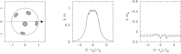
Figures 2 to 5 present illustrative lightcurves for several different configurations of star, lens and spots. In each of these figures we have assumed that the angular radius of the source is equal to the angular Einstein radius of the lens. While this choice of stellar radius is observationally unrealistic and produces low amplification events, for illustrative purposes it has the advantage of producing spot features on the lightcurves which are clearly distinguishable by eye. We will consider somewhat more realistic values of the ratio of stellar radius to Einstein radius later in this section. Lightcurves were computed from the NextGen models in the $U$ to $K$ bands; however for clarity only 4 bands are shown in the following figures. The $V$, $R$, $I$ and $K$ bands are represented by a continuous, a dashed, a dotted and dashed-dotted line respectively.

In Figures 2 to 5 three panels are shown. The left hand panel shows the stellar disk, illustrating the position and size of the starspots and the trajectory (indicated by an arrow) of the lens during the event (in fact all four cases are for a lens impact parameter, $u_{0}=0$). The middle panel indicates the (absolute value of the) change, $\Delta m$, in apparent magnitude as a function of time, as given by the formula

$$\Delta m=\left|2.5\log_{10}\left(\frac{F_{\mathrm{LSP}}}{F_{\mathrm{USP}}}\right)\right|$$ (7)

where $F_{\mathrm{LSP}}$ and $F_{\mathrm{USP}}$ denote the flux from the lensed, spotted star and unlensed spotted star respectively. (Note that, since the effect of lensing is – of course – to amplify the unlensed flux, the sign of the change in apparent magnitude is alwys negative). Similarly the right hand panel shows the change, $\Delta m_{\mathrm{S}}$ in apparent magnitude resulting specifically from the presence of the spot(s), as given by the formula

$$\Delta m_{\mathrm{S}}=-2.5\log_{10}\left(\frac{F_{\mathrm{LSP}}}{F_{\mathrm{LSF}}}\right)$$ (8)

where $F_{\mathrm{LSF}}$ denotes the lensed flux from the spot-free star. (Note that $\Delta m_{\mathrm{S}}$ may be either positive or negative).

While the middle panel indicates the time evolution in observed apparent magnitude of the stellar disk plus spot(s) during the microlensing event, it is difficult to isolate from this panel the contribution to the lightcurve of the spots themselves. Thus, although the final panel indicates a flux ratio which would not be directly observable, it nevertheless makes clear the residual magnitude change between the observed flux from a spotted source and the predicted flux from an event with identical stellar and lens parameters (i.e. stellar radius, atmospheric limb darkening, lens impact parameter etc) but without the non-radial surface brightness variations due to the presence of spots.

Note that $\Delta m_{\mathrm{S}}$ as defined by Equation 8 would give a wavelength dependent non-zero offset, even in the absence of lensing. This arises because the integrated unlensed flux from the spotted star would, in any case, introduce a magnitude change when compared to the unspotted star. Thus we can think of $\Delta m_{\mathrm{S}}$ as composed of two contributions;

$$\Delta m_{\tiny{S}}=\Delta m_{\tiny{SL}}-2.5\log_{10}\left(\frac{F_{\tiny{USP}}}{F_{\tiny{USF}}}\right)$$ (9)

where $F_{\mathrm{USF}}$ denotes the unlensed flux from the spot-free star. Hence $\Delta m_{\mathrm{SL}}$ can be regarded as the magnitude change due to the lensing of the spots, while the second term represents the non-zero offset discussed above. Although we are, of course, primarily interested in $\Delta m_{\mathrm{SL}}$, it is useful to include the non-zero offset in the right hand panels of Figures 2 to 5 as it adds to the clarity of the lightcurve deviations.

Figure 2 illustrates the $V$, $R$, $I$ and $K$ lightcurves produced by the transit of a lens across the disk of a $5000$ K dwarf star and five $4200$ K circular spots of radius $10^{\circ}$. These spot parameters are motivated by, and are broadly consistent with, the results of stellar maps derived from Doppler imaging studies of active dwarfs (see e.g. Strassmeier and Linsky, 1996, and references therein). It can be seen that the two cool spots very close to the lens trajectory are the only features which contribute significantly to the lightcurve. The central spot produces a noticeable ‘dip’ in the central portion of the lightcurve, although the feature becomes less prominent at longer wavelengths and is barely detectable in the $K$ band. This is not surprising as the contrast in limb darkening between $5000$ K and $4200$ K diminishes at longer wavelengths. The spot close to the right hand limb of the star produces a signal of slightly smaller amplitude – although with a similar dependence on wavelength – which is due in part to the geometrical foreshortening clearly visible in the left hand panel.

Note also that the position of this spot, in the ‘wings’ of the light curve, renders it very difficult to isolate in the middle panel, although its presence is obvious in the right hand panel.

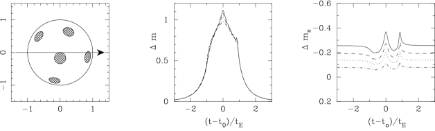
Figure 3 shows the same lens trajectory and configuration of five spots as in Figure 2, but now with a temperature of $4800$ K on a $4000$ K giant star. Here the spot radius and temperature difference is motivated by the HST observations of $\alpha$ Orionis (Gilliland and Dupree 1996). Once again, only the two spots which lie very close to the lens trajectory are ‘imaged’ by the lens, producing a peak in the lightcurves, which diminishes in amplitude at longer wavelengths. Note from the right hand panel that the unlensed offset between different wavebands and the peak magnitude change due to lensing are both somewhat larger than in Figure 2; i.e. the unlensed (and lensed) contrast of hotspots is greater than that of cool spots. This is not surprising, since what is important is the (log) ratio of spotted to unspotted flux; this translates to a larger magnitude change for the hot spot than for the cool spot, although the temperature difference has the same absolute value in both examples.

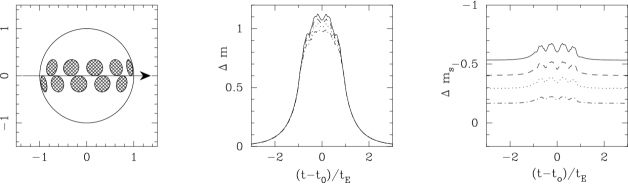
The lensing signature of multiple spots is also interesting, particularly if spots are restricted to a given latitudinal band. Figures 4 and 5 show a $4000$ K giant star with a large group of $4800$ K, $10^{\circ}$ radius spots filling a $40^{\circ}$ band in latitude, straddling the equator. In Figure 4 the inclination of the source star is $90^{\circ}$, so that the lens trajectory intersects the spot bands. We can see from the middle and right hand panels that the spots produce a complex pattern, with a series of ‘bumps’ each one of which is roughly identifiable with an individual spot. The amplitude of each feature, however, varies with spot longitude – due to foreshortening and limb darkening – and also diminishes considerably with increasing wavelength as before.

Another interesting feature is apparent in the right hand panel of Figure 4. We can see in the wings of the light curve that even in the absence of lensing the presence of the large band of spots produces, as one might expect, a substantial magnitude offset which is also strongly wavelength dependent (more than 0.5 mag. at $V$, reducing to less than 0.2 mag. at $K$). In the central part of the lightcurve, as the lens transits the star and crosses the band of spots, the flux in each waveband is amplified due to lensing. Moreover the effect of the lensing is also to increase very slightly the differential magnitude offset in the central part of the light curve, compared with the offset in the wings. However, this differential effect is slightly smaller between the series of ’bumps’ (when the lens is passing through a ’gap’ in the band of spots – e.g. at $t=t_{0}$) than it is at the peaks of the bumps (when the lens is at its closest to one or more of the spots in the band). Thus, the increase in flux due to the presence of the spots (which is augmented by the lens but which would be apparent even if there were no lensing) is slightly diluted when the lens is amplifying the flux from the background star more than the spots themselves.

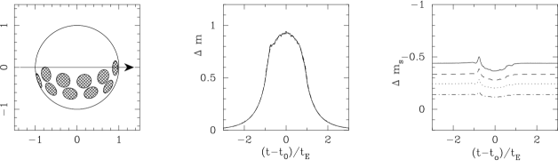
This interplay between the amplified flux from the spots and the background star is more clearly seen in the corresponding panels of Figure 5, which shows the microlensing light curves of the same band of spots, but now on a star of inclination $60^{\circ}$. Again we see a wavelength-dependent magnitude offset even when there is no lensing, due to the presence of the hot spots. Shortly after the stellar transit begins there is a small ’spike’ in the light curves, as the lens passes very close to one of the spots. Thereafter, however, there is a large dip around the central part of each light curve, which also slightly reduces the differential magnitude offset between the wavebands. This is because, during this time, the flux is dominated by the amplified contribution from the region of the star very close to the lens, which – as can be seen from the left hand panel of Figure 5 – is spot free. Thus we see that even when the lens does not pass directly over a spotted region, the presence of spots elsewhere on the star still results in a clearly detectable microlensing signature in the lightcurve as a whole.

The systematic deviations from the unspotted light curves illustrated in Figures 2 to 5 highlight a potential pitfall of estimating stellar and lens parameters from discretely sampled data. In Figure 3, for example, the peak produced by the central spot feature could – if sampled with poor time resolution – lead to the estimation of a stellar radius which was systematically smaller than the true radius. In this respect, in addition to the obvious benefit of increasing the time resolution of observations, multiwavength photometry can also be effective in breaking the apparent degeneracy between a spotted star and a spot-free star of smaller radius. This is because the effect of the starspot is considerably reduced at longer wavelengths. Similar remarks apply to the case of the cool spots on Figure 2, although since the amplitude at a given wavelength of the spot feature is somewhat smaller for cool spots, the (positive) systematic bias in the estimated stellar radius would be less significant than the (negative) bias obtained from higher amplification hotspots.

Figure 4: The $V$, $R$, $I$ and $K$ microlensing light curves produced by the transit of a lens, with impact parameter $u_{0}=0.0AER$, across the disk of a $4000$ K star, of radius 1 $\theta_{E}$, with $\log g=1.0$, with a band of $4800K$ starspots (as shown in the left hand panel) of radius $10^{\circ}$ viewed at an inclination of $90^{\circ}$. The magnitude changes, $\Delta m$ and $\Delta m_{s}$ are as defined in Equations 7 and 8.

Figure 5: The $V$, $R$, $I$ and $K$ microlensing light curves of the same source as in Figure 4 but now viewed at an inclination of $60^{\circ}$.

4.2 Investigating spot detectability

Figure 6: The regions of excess magnification of $0.01,0.05$ and $0.1$ magnitudes from the lightest gray to darkest due to a spot feature of $4800$ K on a 0.1 $\theta_{E}$, $\log g=1.0$, $4000$ K star. Rows from top to bottom correspond to lens trajectories with minimum impact parameter, $u_{0}=0.0,0.4,0.8$ and $1.2$, respectively, normalised to the source radius. Columns from left to right correspond to spots of radius $3^{\circ},6^{\circ},9^{\circ}$ and $12^{\circ}$ respectively.

We next carried out an extensive investigation of spot detectability as a function of spot radius and position and lens impact parameter. These calculations were performed for the somewhat more realistic case of a star with angular radius $R_{*}=0.1\theta_{E}$. This value is comparable to – albeit slightly larger than – the estimated stellar radius for MACHO 95-30 (Alcock et al. 1997), and is similar to the value adopted in the calculations of HS00. There could, of course, be some merit in considering sources of smaller angular radius since MACHO 95-30 represents the largest source star detected to date. Moreover, a smaller source star would also yield a larger microlensing signature. However, given the reduced probability of a point lens transit for such a star – together with the greatly reduced likelihood of intensive photometric monitoring during that transit – we adopt $R_{*}=0.1\theta_{E}$ as a reasonable compromise between considering a star with unrealistically large angular radius and a star with unrealistically low probability of being observed undergoing a point lens transit. (See also Section 5 below).

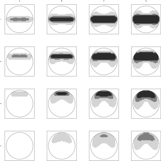
Figure 6 presents $V$ band contour maps of spot detectability for a range of spot and lens parameters. In all cases, the background stellar temperature and spot temperature were taken to be $4000$ K and $4800$ K respectively. Rows from top to bottom correspond to lens trajectories with impact parameter, $u_{0}=0.0,0.4,0.8$ and $1.2$, respectively, normalised to the source radius. Columns from left to right correspond to spots of radius $3^{\circ},6^{\circ},9^{\circ}$ and $12^{\circ}$ respectively.

We assume for each light curve that a total of 80 equally spaced observations were made during $t_{E}$, i.e. the time taken for the lens to move 1 angular Einstein radius. (Hence, for example $t_{E}=40$ days would imply a sampling rate of two observations per day).

The contours shown denote the contribution to the change in magnitude arising specifically from the lensing of the spot, defined as $\Delta m_{\mathrm{SL}}$ in Equation 9 above. The darkest level shown denotes a peak magnitude change of at least 0.1 mag.(i.e. at least one observation for which $\Delta m_{\mathrm{SL}}\geq 0.1$); the lightest level denotes a peak change of 0.01 mag.

It is clear from these contour maps that, as one might expect, the detectability of starspots is improved greatly in regions where the spot lies close to the trajectory of the lens.

Nevertheless, at least for the larger spots, a substantial fraction of the stellar surface would give a detectable signature if a starspot were present at that location. For a spot of radius $12^{\circ}$ and a lens impact parameter $u_{0}=0$, for example, we can see from the top right panel of Figure 6 that the spot would provide a magnitude change of 0.1 mag. or greater over about 30% of the visible disk of the star. We can compare that with the area covered by the spot itself as a fraction of the area of the visible hemisphere, that is $\sin^{2}\delta$, so in this case about 4.3%. Hence microlensing is very efficient at detecting spots under these conditions.

It is interesting to note, however, that even for the case of $u_{0}=0.12\theta_{E}$ (i.e. impact parameter slightly greater than the stellar radius) one still finds that approximately $40$ % of the stellar disk yields a magnitude change in excess of 0.01 mag (compared with the 4% area covered by each spot). Although such a signal would clearly be difficult to detect, its residuals are comparable to the accuracy levels achieved by the best current photometry in microlensing follow up surveys.

The furthest left column of Figure 6 (spot radius of $3^{\circ}$) shows, as expected, the smallest ‘detectable’ regions of the photosphere. Indeed, for $u_{0}=0.12\theta_{E}$ it can be seen that no detectable signal would be obtained. Note also the discrete features in the top left panel (and in a few other panels) which arise because of the small size of the spots and the discrete nature of the the temporal sampling. With more intensive time coverage these features would become more smooth.

It should be stressed, of course, that the contour maps shown in Figure 6 assume that one can predict accurately the unspotted lightcurve – i.e. one can accurately estimate the source radius and lens impact parameter from the lightcurves as a whole. Uncertainty in those parameters would generally impair the sensitivity of the lightcurves to the presence of spots by reducing the detectability area of the contour maps. A detailed investigation of the impact of ‘global’ parameter errors on the estimation of linear limb darkening coefficients from analysis of event OGLE-99-BUL-23 was carried out by Albrow et al. (2001a), and a similar statistical analysis would be important in the context of starspots when confronting real microlensing data. Global parameter errors would clearly have the most damaging effect for small spots, and indeed might ‘wash out’ completely the signature of $3^{\circ}$ spots in the leftmost column of Figure 6. In those regions where the spot signature exceeds 0.1 mag., however, spots would still be easily detectable by current folow up surveys, even allowing for uncertainties in the global parameters.

4.3 The feasibility of gravitational imaging

Figure 7: A comparison of the $V$, $R$, $I$ and $K$ microlensing light curves produced by the transit of a lens, with impact parameter $u_{0}=0.0AER$, across the disk of a $4000$ K star, of radius 1 $AER$, with $\log g=1.0$, with five $4800$ K starspots of radius $10^{\circ}$ (i.e. Figure 2) against an identical source other than additional central temperature structure at $5600$ K of $5^{\circ}$ (as shown in the left hand panel) within the spots. $\Delta A$ is as defined in Equation 10.

We have seen in the previous section that high time resolution observations during a transit event can place useful constraints on the existence or otherwise of spots on particular regions of the photosphere. The question remains as to whether one can constrain the detailed structure of spot features from such observations.

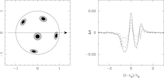
Figure 7 shows a comparison between the light curves produced by the event illustrated in Figure 3 and a similar event, with the same stellar and lens parameters, but in which the spots have additional temperature structure – specifically a central ‘umbra’ of temperature $5600$ K and radius $5^{\circ}$ surrounded by a cooler ‘penumbra’ of temperature $4800$ K (the same temperature as the uniform spots of Figure 3). The right hand panel of Figure 7 shows the difference, in the amplification between the two scenarios, given by

$$\Delta A=\left(\frac{F_{\mathrm{LSP}}}{F_{\mathrm{USP}}}\right)_{\rm struc}\;-\;\left(\frac{F_{\mathrm{LSP}}}{F_{\mathrm{USP}}}\right)_{\rm no-struc}$$ (10)

It is evident from Figure 7 that the effect of the spot structure is small, with a peak deviation from the uniform temperature case of only $\Delta A\simeq 0.02$, which corresponds to $\Delta m\simeq 0.01$ mag. Clearly, then the detection of temperature structure, given the accuracy of current photometry, would be very difficult. A more serious difficulty, however, is presented by the severe ill-posedness of the problem: since spots need not in general be circular it is likely that the specific photometric signature of temperature structure within a circular spot could be closely approximated by a non-circular spot of uniform temperature. In essence, one cannot effectively constrain the 2 dimensional structure of a given spot feature from only a 1 dimensional microlensing light curve. Similar remarks clearly apply to the photosphere as a whole, where groups of (arbitarily shaped) individual spots could mimic the signature of a single, larger, spot and vice versa.

Possible rotation of the source star (which is certainly an area of some interest in the study of red giants and supergiants) is another potential source of degeneracy in the signatures of starspots. Depending on the orientation of the rotation axis with respect to the lens trajectory, a small rotation of the source during the transit of a spot of radius, say, $10^{\circ}$ might broaden or narrow the spot signature in the light curve by an amount equivalent to a change in the spot radius of about $1^{\circ}$. Clearly the magnitude of the effect depends on the star’s rotation period and the lens timescale, but the main point is that – without a precise model for the shape and size of the spot feature – one cannot accurately constrain the rotation period from the spot signature. It is interesting to consider whether the use of multicolour lightcurves might at least partially break the degeneracy between models of spot structure and/or stellar rotation. The practical limitation here, however, is the fact that at longer wavelengths spot signatures are considerably supressed and are less sensitive to surface temperature and other stellar parameters. In future work, we will, nevertheless, investigate optimal methods for combining multicolour data to constrain atmosphere and spot models in this manner.

5 Discussion

The results presented in Section 4 clearly show that the impact of non-uniform surface brightness profiles on the microlensing light curves of point caustic events is, in principle, detectable with current observational precision. There are several important caveats, however.

Firstly, as discussed in Section 4.3, the degenerate nature of the microlensing light curve, which is a convolution over the stellar disk, renders the task of constraining the precise number, position, shape, size and temperature contrast of starspot(s) an ill-posed problem. Notwithstanding these limitations, however, Figure 6 shows that – for a transit or near transit event – a significant fraction of the photosphere will yield an observable magnitude change due to the presence of even a single spot, provided it has sufficient area and temperature contrast. (In fact, since the important quantity in determining the size of the spot signature is the ratio of spotted to unspotted flux, changing the spot temperature contrast is a more important factor than changing the spot area – at least in the wavebands considered here; for the idealised case of black-body radiation and ignoring limb darkening, the spot flux will be proportional to the product of the area and the fourth power of the temperature).

Thus it is clear that the failure to detect a significant deviation from the light curve signature expected for an unspotted source does indeed allow one to place robust limits on the fraction of the stellar disk (i.e. the ‘filling factor’) which could be covered by starspots.

Of course the crucial issue here is not simply the presence or otherwise of spot features, but also one’s ability to detect them.

As we discussed in Section 4.2, an important consideration here is the question of how well determined are the ‘global’ parameters of the event – i.e. the lens minimum impact parameter and the source radius which determine the predicted spot-free lightcurve. These can, in principle, still be determined from the overall light curve shape, and indeed the use of multicolour observations – which we have shown can be an important diagnostic of the properties of the spots – can also improve the accuracy with which the global parameters are determined. However, any significant uncertainty in the global parameters would weaken the constraints on the spot features since the predicted spot-free light curve would be less well determined. A rigorous statistical treatment of the impact of errors in the global parameters would be a crucial step before robust limits on the properties of spots could be inferred from real microlensing data.

The main practical limitation, however, to the use of point lens events as probes of stellar surface features is simply the trajectory of the lens. Spots which lie in regions of the disk far from the lens path will not be readily detected under any circumstance. Even regions lying very close to the lens trajectory, however, would require excellent photometry and high temporal sampling, in order to detect smaller features. In the illustrative example of Figure 6 – for which we assumed a sampling rate of e.g. approximately twice per day for an event with timescale $t_{E}=40$ days – spots smaller than $3^{\circ}$ in radius were undetectable even with a minimum detection criterion of having only one observation with $\Delta m_{\mathrm{s}}\geq 0.1$ mag. Clearly a statistically convincing detection might require several consecutive data points with $\Delta m_{\mathrm{s}}$ greater than some chosen threshold. This could be achieved either through having larger spots (as is indeed the case for the other columns of Figure 6) or by increasing the temporal sampling. While the latter is, of course, always desirable, telescope logistics dictate that – without prior warning that a transit is about to occur – a sampling rate greater than about twice per day is not realistic. Transits of a point mass lens are rare and even for high amplification events, difficult to predict from the pre-transit lightcurve. A more ‘observationally friendly’ scenario is the transit of an extended source by the caustic structure produced by a binary lens. This is because in such a high amplification microlensing event it becomes necessary to treat every source as an extended source and hence the source’s surface brightness profile can be investigated. Furthermore the intial transit ‘into’ the structure acts as a alert, allowing intensive observations of the second crossing ‘out of’ the structure to be planned. Such ‘alert response’ photometry is currently being carried out with the aim of detecting low-mass companions but clearly has scope to image stellar atmospheres, allowing the detection or otherwise of photospheric starspots. Gravitational imaging by non-point lens objects will be addressed in a forthcoming paper.

Appendix A Starspot geometry and integration limits

A.1 Coordinate systems

We calculate the integrated flux from the star, in both the lensed and unlensed case, in terms of an integral over the projected stellar disk. There are three coordinate systems relevant to this calculation:

1. $(\alpha^{\prime},\phi^{\prime})$ : spherical polar coordinates on the surface of the star, with the stellar equator defining $\phi^{\prime}=0$, and with $\alpha^{\prime}$ measured counter-clockwise from the direction which is co-planar with the star’s rotation axis and the line of sight (as shown in Fig. A1).

2. $(\alpha,\phi)$ : spherical polar coordinates on the surface of the star, but with polar axis $(\phi={\pi\over 2})$ defined as the projection of the star’s rotation axis on the plane of the sky and with azimuthal angle, $\alpha$, measured counter-clockwise from the line of sight (as shown in Fig. A2).

3. $(s,\theta)$ : projected circular polar coordinates on the stellar disk (i.e. the plane of the sky), with $\theta$ measured counter-clockwise from the $y$-axis (see below).

Figures A1 and A2 illustrate these coordinate systems and their associated Cartesian coordinate axes. Thus, we define the $x$-axis to be the line of sight, the $z$-axis to be the projection of the star’s rotation axis onto the plane of the sky, and the $y$-axis to be the direction which completes a right-handed coordinate system. It is then easy to see that the $y$-axis and $y^{\prime}$-axis are identical, and the $x^{\prime}$-axis and $z^{\prime}$-axis are obtained from the $x$-axis and $z$-axis by a rotation of $({\pi\over 2}-i)$ about the $y$-axis, where $i$ is the inclination of the star. In summary, for a star of radius, $R$, and a general point $(x,y,z)$ on the stellar surface

$$x = R\cos\alpha\cos\phi\,\,=\,\,R(\cos\alpha^{\prime}\cos\phi^{\prime}\sin i+\sin\phi^{\prime}\cos i)$$

$$y = R\sin\alpha\cos\phi\,\,=\,\,R\sin\alpha^{\prime}\cos\phi^{\prime}$$

$$z = R\sin\phi\,\,=\,\,R(\sin\phi^{\prime}\sin i-\cos\alpha^{\prime}\cos\phi^{\prime}\cos i)$$ (11)

where all coordinates are expressed in units of the angular Einstein radius (AER) of the lens.

Figure 8: Spherical polar coordinates on the surface of the star, with the stellar equator defining $\phi^{\prime}=0$, and with $\alpha^{\prime}$ measured counter-clockwise from the direction which is co-planar with the star’s rotation axis and the line of sight.

Figure 9: Spherical polar coordinates on the surface of the star, but now with polar axis $(\phi={\pi\over 2})$ defined as the projection of the star’s rotation axis on the plane of the sky and with azimuthal angle, $\alpha$, measured counter-clockwise from the line of sight

Consider now the path of a point lens, as seen in projection on the sky. Figure 10 shows the lens trajectory and the position of the lens at some general point, $L$, and at time, $t$. Here, $u$ denotes the impact parameter of the lens and $u_{0}$ denotes the impact parameter at the time of closest approach, $t_{0}$, when the lens has position angle $\theta_{0}$, as shown. Let $t_{E}$ denote the time for the lens to move $1\theta_{E}$. The coordinates $(y_{\tiny{\rm{L}}},z_{\tiny{\rm{L}}})$, of the lens at position, $L$, are

$$y_{\tiny{\rm{L}}} = u_{0}\cos\theta_{0}-\frac{(t-t_{0})}{t_{E}}\sin\theta_{0}$$

$$z_{\tiny{\rm{L}}} = u_{0}\sin\theta_{0}+\frac{(t-t_{0})}{t_{E}}\cos\theta_{0}$$ (12)

The projected separation, $u$, of the lens from an arbitrary point, $(y,z)=(s\cos\theta,s\sin\theta)$, on the stellar disk is

$$u=\left[(y_{\tiny{\rm{L}}}-s\cos\theta)^{2}+(z_{\tiny{\rm{L}}}-s\sin\theta)^{2}\right]^{1/2}$$ (13)

Figure 10: Lens trajectory

A.2 Defining the boundary of a circular starspot

We consider circular starspots – i.e. the locus of points defining the boundary of a spot is a small circle of angular radius $\delta$, say. We suppose that each starspot maintains constant radius, temperature and latitude (in the stellar-based coordinate system) throughout the microlensing event, but that its longitude changes if the star is rotating.

Let $({\alpha_{p}}^{\prime},{\phi_{p}}^{\prime})$ denote the (stellar-based) coordinates of the centre of the starspot. If the star is not rotating, these coordinates remain fixed; if the star is rotating with period, $P$, and the spot centre transits at time, $t_{0}$, then

$${\alpha_{p}}^{\prime}=\frac{2\pi}{P}(t-t_{0})$$ (14)

We can easily obtain from eqs. 11 the projected circular polar coordinates, $(s_{p},\theta_{p})$, of $P$ in the observer-based coordinate system. The circumference of the spot describes a planar circle of radius $R\sin\delta$. The centre, $C$, of this circle lies inside the star, i.e.

$$x_{c} = R\cos\delta\cos\alpha_{c}\cos\phi_{c}$$

$$y_{c} = R\cos\delta\sin\alpha_{c}\cos\phi_{c}\,\,=\,\,s_{c}\cos\theta_{c}$$

$$z_{c} = R\cos\delta\sin\phi_{c}\,\,=\,\,s_{c}\sin\theta_{c}$$ (15)

Note that $s_{c}=s_{p}\cos\delta$ and $\theta_{c}=\theta_{p}$.

Thus, when seen in projection the centre, $C$, of the planar circle defining the spot boundary is not coincident with the centre, $P$, of the spot on the surface of the star, but does lie along the same radial vector joining $P$ to the centre of the stellar disk.

Consider a general point $(x,y,z)$ on the circumference of the spot. We have

$$(x-x_{c})^{2}+(y-y_{c})^{2}+(z-z_{c})^{2}=R^{2}\sin^{2}\delta$$ (16)

and

$$x^{2}+y^{2}+z^{2}=R^{2}$$ (17)

Combining eqs. 16 and 17 gives, after some manipulation

$$xx_{c}+yy_{c}+zz_{c}=R^{2}\cos^{2}\delta$$ (18)

which, as expected, defines a plane perpendicular to the position vector $(x_{c},y_{c},z_{c})$.

A.3 Spot visibility conditions

Consider a unit vector in the direction of the spot centre, $C$. i.e.

$${\hat{n}}_{c}=(\cos\alpha_{c}\cos\phi_{c},\sin\alpha_{c}\cos\phi_{c},\sin\phi_{c})$$ (19)

Let $\eta$ be the angle between the line of sight and ${\hat{n}}_{c}$. Then $\cos\eta=\cos\alpha_{c}\cos\phi_{c}$. A spot will be fully visible provided $\eta\leq{\pi\over 2}-\delta$, i.e.

$$\cos\alpha_{c}\cos\phi_{c}\geq\sin\delta$$ (20)

Similarly the spot will be fully invisible provided

$$\cos\alpha_{c}\cos\phi_{c}\leq-\sin\delta$$ (21)

and partially visible when

$$-\sin\delta\leq\cos\alpha_{c}\cos\phi_{c}\leq\sin\delta$$ (22)

A.4 Spot centred on the limb of the star

Suppose first that $x_{p}=0$. It is straightforward to show that the spot circumference appears in projection as a straight line perpendicular to the radius vector to $(y_{c},z_{c})$ and the integration limits are

$$\theta_{c}-\delta\leq\theta\leq\theta_{c}+\delta\quad\quad\quad\frac{R\cos\delta}{\cos(\theta-\theta_{c})}\leq s\leq R$$ (23)

A.5 Fully visible spot

Suppose now that $x_{c}\neq 0$. For a fully visible spot, at any time the projected spot will appear as an ellipse centred on $(y_{c},z_{c})$. The semi-major axis is perpendicular to the radius vector to $(y_{c},z_{c})$ and some straightforward algebra shows that it has length $l_{1}=R\sin\delta$. To determine the semi-minor axis we require to solve for the value(s) of $s$ at which the spot projection intersects the radius vector through $(y_{c},z_{c})$. Clearly, at the points of intersection we have

$$y=s\cos\theta_{c}\quad\quad\quad z=s\sin\theta_{c}$$ (24)

From eq. 18 it follows that

$$x=\frac{R^{2}\cos^{2}\delta-yy_{c}-zz_{c}}{x_{c}}$$ (25)

Combining eqs. 17 and 25 gives

$$(R^{2}\cos^{2}\delta-yy_{c}-zz_{c})^{2}+y^{2}x_{c}^{2}+z^{2}x_{c}^{2}=R^{2}x_{c}^{2}$$ (26)

which, substituting from eqs. 15 and 24, may be reduced to the quadratic equation in $s$

$$R^{2}\cos^{2}\delta-2s_{c}s+s^{2}-R^{2}\cos^{2}\alpha_{c}\cos^{2}\phi_{c}=0$$ (27)

This has determinant, $\Delta$, which some algebra reduces to

$$\Delta=4R^{2}\cos^{2}\alpha_{c}\cos^{2}\phi_{c}\sin\delta$$ (28)

Hence eq. 27 has roots

$$s=s_{c}\pm R\cos\alpha_{c}\cos\phi_{c}\sin\delta$$ (29)

from which we see immediately that the projected spot ellipse has semi-minor axis $l_{2}=R\cos\alpha_{c}\cos\phi_{c}\sin\delta$.

We can parametrise a general point inside this ellipse as

$$y_{E}=\omega\,l_{1}\,\cos\theta_{E}\quad\quad\quad z_{E}=\omega\,l_{2}\,\sin\theta_{E}$$ (30)

Where $0\leq\omega\leq 1$ and $0\leq\theta_{E}\leq 2\pi$. The coordinates $(y_{E},z_{E})$ are related to $(y,z)$ via

$$y = y_{E}\sin\theta_{c}+z_{E}\cos\theta_{c}+s_{c}\cos\theta_{c}$$

$$z = z_{E}\sin\theta_{c}-y_{E}\cos\theta_{c}+s_{c}\sin\theta_{c}$$ (31)

The integral in eq. 17 may then be expressed in terms of $\omega$ and $\theta_{E}$, viz

$$\Delta F=l_{1}l_{2}\int_{\theta_{E}=0}^{2\pi}\int_{\omega=0}^{1}\left[I_{\rm{sp}}(s,\theta)-I_{*}(s)\right]\,A(d)\,\omega\,d\omega d\theta_{E}$$ (32)

A.6 Partially visible spot

The case where a spot is only partially visible is slightly more complicated. Consider the intersection of the projected spot ellipse with a circle of radius $s$ on the stellar disk and centered on $O$. Putting $y=s\cos\theta$, $z=s\sin\theta$, $y_{c}=s_{c}\cos\theta_{c}$, $z_{c}=s_{c}\sin\theta_{c}$ and substituting in eq. 18, gives, after some further reduction

$$\cos(\theta-\theta_{c})=\frac{R^{2}\cos^{2}\delta-x_{c}\sqrt{R^{2}-s^{2}}}{ss_{c}}$$ (33)

or, writing in terms of $\alpha_{c}$ and $\phi_{c}$,

$$\theta=\theta_{c}\pm\cos^{-1}\left[\frac{R\cos\delta-\cos\alpha_{c}\cos\phi_{c}\sqrt{R^{2}-s^{2}}}{s(\sin^{2}\alpha_{c}\cos^{2}\phi_{c}+\sin^{2}\phi_{c})^{1/2}}\right]$$ (34)

Thus, for a partially visible spot we integrate eq. 17 using the limits

$$s_{c}-R\cos\alpha_{c}\cos\phi_{c}\sin\delta\leq s\leq R$$ (35)

for $s$ and using eq. 34 to define the corresponding limits of $\theta$.

References

- [1] Albrow M., et al., 2001b, ApJ, 549, 759
- [2] Albrow M., et al., 2001a, ApJ, 550, 173
- [3] Alcock C., et al., 1997, ApJ, 486, 697
- [4] Bogdanov M.B., Cherepashchuk, 1995, Astron. Rep., 39, 873
- [5] Bogdanov M.B., Cherepashchuk, 1996, Astron. Rep., 40, 713
- [6] Bontz R.J., 1979, ApJ, 233, 402
- [7] Bryce H. M., Hendry M. A., Valls-Gabaud D., 2002, in ’Microlensing 2000: A New Era of Microlensing Astrophysics’, J.W. Menzies and P.D. Sackett eds., ASP Conf. Ser. 239, 195 (ASP: San Francisco)
- [8] Dorren J.D., 1987, ApJ, 320, 756
- [9] Gaudi B. S., Gould A., 1997, ApJ, 482, 83
- [10] Gilliland R. L., Dupree A. K., 1996, ApJ, 463, L29
- [11] Gould A., 1994, ApJ, 421, 71
- [12] Gould A., 1995, ApJ, 441, L21
- [13] Gould A., 1997, ApJ, 483, 989
- [14] Gould A., Welch D. L., 1996, ApJ, 464, 212
- [15] Gray D.F., 1992, The Observation and Analysis of Stellar Photospheres, (CUP: Cambridge)
- [16] Gray N., Coleman I. J., 2002, in ’Microlensing 2000: A New Era of Microlensing Astrophysics’, J.W. Menzies and P.D. Sackett eds., ASP Conf. Ser. 239, 204 (ASP: San Francisco)
- [17] Han C., Park S.-H., Kim H.-I., Chang K., 2000, MNRAS, 316, 97
- [18] Hauschildt P.H., Allard F., Baron E., 1999, ApJ, 512, 377
- [19] Hauschildt P.H., Allard F., Ferguson J., Baron E., Alexander D.R., 1999, ApJ, 525, 871
- [20] Hendry M. A., Coleman I. J., Gray N., Newsam, A. M., Simmons, J. F. L., 1998, New Astronomy Reviews, 42, 125.
- [21] Heyrovský, D., Loeb, A., 1997, ApJ, 490, 38
- [22] Heyrovský D., Sasselov D., 2000, ApJ, 529, 69
- [23] Heyrovský D., Sasselov D., Loeb A., 2000, ApJ, 543, 406
- [24] Ignace R. Hendry M. A., 1999, Astron. Astrophys., 341, 201
- [25] Kurucz R.L., 1994, ATLAS9 CDROMs
- [26] Maoz D., Gould A., 1994, ApJ, 425, 67
- [27] Menzies J. W. and Sackett P. D., (eds.), 2001, Microlensing 2000: A New Era of Microlensing Astrophysics. ASP Conf. Ser. in press (ASP: San Francisco)
- [28] Nemiroff R. J., Wickramasinghe W., 1994, ApJ, 424, 21
- [29] Paczyński B., 1996, Ann. Rev. Aston. Astrophys., 34, 419
- [30] Peng E. W., 1997, ApJ, 475, 43
- [31] Sasselov D., 1997, in Variable Stars and the Astrophysical Returns of the Microlensing Surveys, ed. R. Ferlet et al., (Paris: Ed. Frontières), p. 141
- [32] Simmons J.F.L., Newsam A.M., Willis J.P., 1995, MNRAS, 276, 182
- [33] Simmons J. F. L., Willis J. P., Newsam A. M., 1995, A & A, 293, L46
- [34] Strassmeier K.G., Linsky J.L. (eds), 1996, IAU Symp. 176, Stellar surface structure, (Dordrecht: Kluwer)
- [35] Uitenbroek H., Dupree A. K., Gilliland R, L., 1998, ApJ, 116, 2501
- [36] Valls-Gabaud D., 1994, in Large Scale Structures in the Universe, eds. J. Mücket et al., (Singapore: World Scientific), p. 326
- [37] Valls-Gabaud D., 1996, in Astrophysical applications of gravitational lensing, IAU Symp 176, eds. C. S. Kochanek and J.N. Hewitt, (Dordrecht: Kluwer), p. 237
- [38] Valls-Gabaud D., 1998, MNRAS, 294, 747
- [39] Vermaak P., 2000, MNRAS, 319, 1011
- [40] Witt H.A., Mao S., 1994, ApJ, 430, 505
- [41] Witt H.A., 1995, ApJ, 449, 42