Multi–frequency Analysis of the two CSS quasars
3C 43 & 3C 298

We present and discuss observations made with MERLIN and VLBI at 1.7 and 5 GHz of the two CSS quasars 3C 43 and 3C 298. They show quite different morphologies, the former being a very distorted triple radio source, the latter a small FRII type object. Relativistic effects and structural distortions are discussed. Source ages are evaluated to be of the order of $\approx 10^{5}$ years, therefore 3C 43 and 3C 298 can be considered fairly “young” radio sources. Some inference is also derived on the properties of the medium surrounding the radio emitting regions in these sub–galactic objects, whose density could be as low as 10^-3 cm^-3.

1 Introduction

Compact Steep–spectrum Sources (CSS) and GHz Peaked spectrum Sources (GPS) are powerful objects whose projected sizes are shown, statistically (Fanti et al. fan3 (1990)), to be physically small ($<15-20\leavevmode\nobreak\ h^{-1}$ kpc). Their high–frequency spectrum is steep (and turns over at low frequencies in GPS) implying that these objects are not core dominated. When observed with the appropriate resolution they display a large variety of morphologies. Their nature has been a matter of debate for many years and several samples of CSSs and GPSs have been studied by numerous authors in an effort to understand their properties and their rôle in the radio source evolution. General discussions have been presented, for instance, by Fanti et al. (fan1 (1985)), Saikia (saik (1988)), Fanti et al. (fan3 (1990)), Spencer et al. (spen2 (1991)), Fanti et al. (fan5 (1995)), Readhead et al. (read (1996)), O’Dea & Baum (ode2 (1997)). An extensive review has been presented by O’Dea (ode (1998)).

It is now generally accepted that at least a large fraction of CSSs/GPSs are young radio sources in the early stage of their life ($\mathrel{<\kern-10.00002pt\lower 3.87495pt\hbox{$\sim$}}10^{6}$ years; see e.g. Fanti fan6 (2000) for a short review) and statistical studies of CSSs and GPSs are therefore important in order to refine the evolutionary scenario. Extensive studies of individual objects are also important, however, in order to understand the underlying physics. Moreover, due to their small physical sizes, these objects may give us an unique opportunity to probe the interstellar medium (ISM) of their host galaxy/quasar and, in the smallest of them, even the Narrow Line Region (NLR ) via jet–ambient gas interactions (see for instance de Vries, devr (1999), Conway & Schilizzi, con2 (2000), Axon et al. axon (2000) and references therein, Morganti et al. morg (2001)).

In this paper we present a detailed study of the CSS quasars 3C 43 and 3C 298 based on different resolution images we obtained using MERLIN and VLBI at 1.7 and 5 GHz and complemented by images at other frequencies. These quasars have similar redshift and radio power but very different radio morphologies: 3C 43 shows a very distorted structure; 3C 298, instead, has an almost linear morphology and appears to be a scaled down version of the large size quasars.

In the following sections we summarize the observations and the data reduction (Sect. 2), present the observational results (Sect. 3) and discuss the properties of both sources (Sect. 4). Finally, in Sect. 5 we provide a summary of the results and some conclusions.

2 Observations and Data reduction

Table 1: Observational information for 3C 43 and 3C 298

source	$\nu$(GHz)	date	Obs. Mode	Stations
3C 43	1.7	1993.60	MERLIN	Jodrell(MK2), Darnhall, Defford, Knockin, Tabley, Wardle, Cambridge,
		1986.75	MKII	Onsala, Medicina, Defford, Effelsberg, Westerbork, Lovell
	5.0	1991.70	MERLIN	Jodrell (MK2), Knockin, Darnhall, Defford, Tabley
			MKII	Effelsberg, Westerbork, Jodrell(MK2), Knockin, Cambridge
			MIIIB	Effelsberg, Westerbork, Jodrell(MK2), Onsala
3C 298	1.7	1982.82	MERLIN	Jodrell(MK2), Darnhall, Defford, Knockin, Tabley, Wardle
		1991.88	MKII	Effelsberg, Westerbork, Torun, Crimea, Lovell, Medicina,
				Green Bank, Y27, OVRO, VLBA_(NL, FD, LA, PT, KP)
	5.0	1983.66	MERLIN	Jodrell(MK2), Knockin, Darnhall, Defford, Tabley
		1992.24	MKII	Cambridge, Effelsberg, Jodrell(MK2), Knockin, Medicina
			MKIIIB	Effelsberg, Jodrell(MK2), Medicina, Noto, Onsala, Westerbork

The new observations presented in this paper were obtained with VLBI networks in different observing modes (MkII and MkIII) and with MERLIN, in the period 1991–1994 at the frequencies of 1.7 and 5 GHz (Table 1).

At 5 GHz the observations of 3C 43 were performed simultaneously with MERLIN and EVN while for 3C 298 we obtained EVN observations only. The EVN observing time was 12 hours for each source and included short scans on the calibration sources 0133+476, 0235+164 and OQ208, about every four hours.

At 1.7 GHz we performed for 3C 298 a global ($EVN+US+VLBA$) observation. The observing time was about 12 hours on both the European and the US networks with only four hours in common to the two networks due to the low source declination. For 3C 43 the EVN data by Spencer et al. (spen2 (1991)) were re-analyzed and a new image is presented here.

Given the complex structure of these sources the use of the combined VLBI and MERLIN data was necessary in order to obtain a good sampling of both the short and the long baselines. As said above, only for 3C 43 at 5 GHz we did manage to have simultaneous observations on the two arrays. The other MERLIN data were: for 3C 43 at 1.7 GHz from observations performed in 1993 with the extended array (i.e. including the 32-m telescope at Cambridge); for 3C 298 pre–existing data by Spencer at al. (spen (1989)) at 1.7 GHz and by Akujor et al. 1991b at 5 GHz.

In order to combine the VLBI and the MERLIN data sets properly, at least one common baseline is highly desirable to link the phases and the flux density scales. This was not possible for 3C 298 at 1.7 GHz. In this case the MERLIN and VLBI data were combined after carefully checking that the “a–priori” flux density scales of the two arrays were in agreement.

The whole data reduction was made in AIPS. The final combined images were obtained by initially mapping and phase self-calibrating the short baseline data and then by slowly adding increasingly longer baselines. For both sources we analyzed images made at different resolutions; they are referred to in the text as low, intermediate and high (see Tables 3 and 5).

3 Results

Some basic parameters for the two quasars 3C 43 and 3C 298 are given in Table 2.

Table 2: Basic information for 3C 43 and 3C 298

source	$z\leavevmode\nobreak\ \leavevmode\nobreak\$	mv	S1.7	S5.0	logP1.7	LS	$\nu_{\rm max}$	$\alpha$
			(Jy)	(Jy)		(kpc $\leavevmode\nobreak\ h^{-1}$)	MHz
3C 43	1.46	20.0	2.6	1.1a	27.83	$\approx 15\ \ \ \ \$	$<$30	0.71
0127+233
3C 298	1.44	16.8	4.9a	1.5b	28.24	6.5	80	1.10
1416+067

$z$: redshift; m_v: visual magnitude; ${\rm S}_{5.0},{\rm S}_{1.7}$: total flux density at the quoted frequency; ${\rm P}_{1.7}$ in W/Hz $h^{-2}$; LS: overall linear size; $\nu_{\rm max}$: observed spectral turnover frequency; $\alpha$: overall spectral index for $\nu\mathrel{>\kern-10.00002pt\lower 3.87495pt\hbox{$\sim$}}$100 MHz, defined as S$(\nu)\propto\nu^{-\alpha}$

$a$ – Spencer et al. (spen (1989)); $b$ – NED

The two sources have been analyzed in similar ways following this scheme:

Figure 1: 3C 43 at 18 cm: (a) MERLIN image ($220\times 145$mas); contours: ($\pm 2\times 2^{n},n\geq 0$) mJy/beam; $S_{\rm peak}=$1.06 Jy/beam; (b) EVN image ($25\times 20$mas) of the “Central” component or bright jet; contours: ($\pm 4.0\times 2^{n},n\geq 0)$ mJy/beam; $S_{\rm peak}=$0.308 Jy/beam

• The source morphology was studied by comparing the images of the present paper with others available in the literature. For the individual components of each source we report in Tables 4 and 6 flux density and beam–deconvolved sizes (HPW), derived using the AIPS task IMFIT. When components cannot be reliably approximated by two–dimensional Gaussians, flux densities have been measured by integration over the emission region (AIPS task TVSTAT) and sizes may have been estimated from the lowest reliable contour in the image. Note that in this case sizes are roughly twice the conventional HPW. Parameters estimated in such a way are preceeded by “$\sim$”.

• On the assumption of minimum energy conditions, we computed for each source component the physical parameters, i.e.: equipartition magnetic field (H_eq), minimum energy density (u_min), minimum total energy (U_eq), turnover frequency ($\nu_{\rm to}$) expected from synchrotron self–absorption. We used standard formulae (e.g. Pacholczyk, pach (1970)), with filling factor 1, equal energy in electrons and protons and an ellipsoidal geometry for sub–components.

• Component radio spectra are derived by combining our own data with those from images in the literature at resolutions not too different from ours.

3.1 3C 43

3.1.1 Source Morphology – Observed and Physical Parameters

At sub–arcsec resolution (Pearson et al. pear (1985); Akujor et al. 1991a , Spencer et al. spen (1989); Akujor & Garrington aku3 (1995)) the morphology is that of a very distorted triple source, with a very bright central component and two outer components, toward East and North–West, whose arms form an angle of $\approx 95^{\circ}$. In the 18 cm image obtained with the extended MERLIN (Fig. 1a) the north–western component is clearly double and the component to East is elongated towards the central one and connected to it. At higher resolutions (van Breugel et al. vanb (1992), Lüdke et al. lud (1998)) the latter component appears as a faint jet which widens at the eastern end in a sort of lobe (see also Fig. 2). No compact features which could be interpreted as “hot–spots” are visible within the eastern or north–western lobes at either frequency, even in the high resolution EVN images.

In the discussion of the source properties we refer to the labelling of Figs. 1 and 2. In these figures: $NW$, “Eastern” and “Central” are the north-western, the eastern and the central components seen at MERLIN resolution (Fig. 1a); $EAST$ and faint jet are the easternmost lobe and the elongated weak structure which connects it to the “Central” component (Fig. 2); bright jet is the “Central” component as seen at VLBI resolutions (Figs. 1b and 4). Here components are labelled from $A$ (North) to $F$ (South–East).

The general parameters of our own high and low resolution VLBI images at 1.7 (Figs. 1b and 2) and at 5 GHz (Fig. 4) are given in Table 3.

Table 3: Image characteristics for 3C 43

	1.7 GHz			5 GHz
resol.	beam	Flux‡	noise†	beam	Flux‡	noise†
	(mas)	(Jy)	(mJy/b)	(mas)	(Jy)	(mJy/b)
high	25$\times$20	1.07	1.3	15$\times$10	0.49	1.0
low	40$\times$40	2.48	1.2	25$\times$17	0.88	0.9

${\dagger}$ noise computed far from the source

${{\ddagger}}$ flux density in the image; at 1.7 GHz low resolution it includes lobe $NW$. The difference in flux density, at both frequencies, between the high and low resolution images is due to the missing short (MERLIN) baselines in the former case, which causes loss of extended low brightness features (see Figs. 1, 2, 4)

Figure 2: 3C 43: EVN+MERLIN image at 18 cm of the “Central” and “Eastern” [$EAST+$ faint jet] components ($40\times 40$mas); contours: ($\pm 2.5\times 2^{n},n\geq 0)$ mJy/beam; $S_{\rm peak}=$0.431 Jy/beam

Figure 3: 3C 43: EVN image at 92 cm ($40\times 40$mas) of the same region as in Fig. 2; contours: ($\pm 2.0\times 2^{n},n\geq 0)$ mJy/beam; $S_{\rm peak}=$1.025 Jy/beam

The low resolution image at 1.7 GHz shown in Fig. 2 is the only one where the faint jet is clearly visible. Component $NW$ (out of figure) is instead just barely detected. This image accounts for $\approx$95% of the total MERLIN flux density. A global VLBI image at 327 MHz of the “Central” and “Eastern” components (component $NW$ is heavily resolved out), with a resolution of $40\times 40$ mas (Dallacasa et al. unpublished) is shown in Fig. 3 for comparison. Most of the structure visible in Fig. 2 can be recognized here.

In the high resolution images presented in Figs. 1b and 4a, only the “Central” component is visible. It appears as a bright jet running initially in the N–S direction, with small oscillations and then sharply bent towards East (see also the 610 MHz image by Nan et al. 1991b , resolution $30\times 20$ mas). Only $\approx 55$% of the flux density measured at 1.7 GHz with MERLIN and $\approx 50$% of that measured at 5 GHz with the VLA by Spencer et al. (spen (1989)) is present in these images. More flux density is detected in the combined EVN$+$MERLIN image at 5 GHz shown in Fig. 4b, thanks to the better coverage of the short baselines. Here $\approx$90% of the VLA flux density of the “Central” component (Spencer et al. spen (1989)) has been recovered.

The 5 GHz low resolution image (Fig. 4b) compares reasonably well with the image at 1.7 GHz (Fig. 1b), with a similar resolution, although the match is not completely satisfactory. In particular the extended structure $C1$ appears more “knotty” here and components $E$ and $F$ are now blended into a single blob. We note that component $A$ (Fig. 1b), brighter at high frequencies, is just barely visible at 327 MHz, heavily blended with component $B$. We estimate that its flux density is not greater than $\approx$20 mJy at this frequency. This provides evidence that it has an inverted spectrum (Sect. 3.1.2) and that it is therefore likely to harbor the source core, as suggested already by Nan et al. (1991b )

Figure 4: the bright jet of 3C 43 at 6 cm: (a) EVN image ($15\times 10$mas); contours: ($\pm 2.0\times 2^{n},n\geq 0)$ mJy/beam; $S_{\rm peak}=$0.131 Jy/beam; (b) EVN+MERLIN image ($25\times 17$mas); contours: ($\pm 2.0\times 2^{n},n\geq 0)$ mJy/beam; $S_{\rm peak}=$0.158 Jy/beam

Table 4: Observed and Derived Parameters for 3C 43

	1.7 GHz	5 GHz			Physical Parameters
comp	S	S	$\theta_{1}\times\theta_{2}$	d${}_{1}\times$d2	$\alpha_{\rm thin}$	H${}_{\rm eq}\ \$	u${}_{\rm min}\ \ \ \$	U${}_{\rm eq}\ \$	$\nu_{\rm to}$
	mJy	mJy	mas	pc $\leavevmode\nobreak\ h^{-1}$		mG	erg/cm${}^{3}\leavevmode\nobreak\ h\ \$	1054erg $h^{-2}$	MHz
A	43	61	17$\times$11	73$\times$47
	–	26	unres.
B	202	121	7$\times$6	30$\times$26	0.54	7.8	5.7$\times 10^{-6}$	10	436
	–	152	8$\times$3
C1	$\sim$90	$\sim$65	39$\times$21	167$\times$90	0.30	1.8	3.0$\times 10^{-7}$	36	81
–		$\sim$40	10$\times$4
C2	$\sim$180	$\sim$80	30$\times$23	129$\times$99	0.63	2.4	5.2$\times 10^{-7}$	57	142
	–	$\sim$30	22$\times$6
D	459	275	20$\times$16	86$\times$69	0.48	4.0	1.5$\times 10^{-6}$	54	252
	–	175	15$\times$10
E+F	$\sim$200	108	28$\times$26	120$\times$111	0.66	2.4	5.1$\times 10^{-7}$	68	145
	–	–	–	–
$NW{\dagger}$	$\sim$185	50	400$\times$300	(1.7$\times 1.3)\times 10^{3}$	$\sim$ 1.1	0.4	1.5$\times 10^{-8}$	3600	32
“Eastern”${\dagger}$	$\sim$560	130	600$\times$300	(2.5$\times 1.3)\times 10^{3}$	1.27	0.6	3.5$\times 10^{-8}$	13000	48

At 5 GHz data on the first line are from the low resolution image, the others from the high resolution image.

${\dagger}$ Data at 5 GHz from Spencer et al. (spen (1989));

$\alpha_{\rm thin}$ spectral index in the frequency range 0.3–5 GHz; H_eq equipartition magnetic field; u_min minimum energy density; U_eq minimum energy; $\nu_{\rm to}$ computed self–absorption turnover frequency (except for $A$)

The EVN observations at 1.7 GHz were performed in September 1986 and those at 5 GHz in September 1991: this represents a time lag long enough to impose the exercise of checking if the source structure has somehow changed. To do this, we have convolved the 6 cm low resolution image to the resolution of the 18 cm (25$\times$20 mas; not shown). We find that all components from $B$ to $D$ appear to have systematically moved away from $A$ (assumed stationary) along PA$\approx-140^{\circ}$, the positional shifts being in the range 3.8–12.5 mas. These displacements are significant and, taken at face value, would imply an apparent outward speed $\beta_{\rm app}\geq 22c$.

Such displacements may be explained as a sort of “reflex motion” due to spectral index and resolution effects within component $A$. In effect $B$ and $D$, the two strongest and most reliable components, have not moved appreciably with respect to each other. If we then take as coordinate origin the position of $B$ instead of $A$, we find that the displacement of $A$ with respect to $B$ increases systematically when we use the 18 cm high resolution, the 6 cm low resolution and the 6 cm high resolution images. This systematic behaviour is consistent with the assumption that $A$ be actually composed by an inverted spectrum compact “true core” (dominating at 6 cm high resolution) at the eastern end of a mini–jet with a normal spectrum, pointing towards $B$ (dominating at 18 cm). Due to the different spectral indices, the relative weight of these two components changes depending on the observing frequency and resolution, and the position of $A$ shifts with respect to $B$ in a way consistent with what observed. Such a sub–structure, confirmed by a recent unpublished VLBA image at 8.4 GHz by Mantovani (private communication), could help in explaining some of the points discussed in Sect. 4.3.

Finally, by comparing the VLA polarization information at 5 GHz (Akujor et al. 1991a ), 8.4 GHz (Akujor & Garrington, aku3 (1995)) and 15 GHz (van Breugel et al. vanb (1992)) we find that both the “Eastern” and the “Central” components show a fair amount of depolarization between 15 and 5 GHz, while the $NW$ component is not depolarized between 8.4 and 5 GHz. Faraday rotation does not seem to be important. The high resolution polarization images by Lüdke et al. (lud (1998)) and by van Breugel et al. (vanb (1992)) show that the magnetic field is well aligned parallel to the bright and the faint jet and follows the bend at $D$.

Observed component parameters are given in Table 4. At 1.7 GHz no sizes are given for components $A$ to $F$ since they are not significantly different from the old ones by Spencer et al. (spen2 (1991)). At 5 GHz we give flux densities and sizes from both the low and the high resolution images, except for the $NW$ and “Eastern” components, whose data are from Spencer et al. (spen (1989)). The derived physical parameters are also reported in Table 4, except for $A$ which is unresolved with an inverted spectrum (Sect. 3.1.2).

3.1.2 Spectral Analysis

The overall spectrum of 3C 43 derived from low resolution data (Kuhr et al. kuh (1981); Steppe et al. step (1995)) is straight with $\alpha=$0.71 from $\approx$30 MHz to 230 GHz.

The addition to the present data of the measurements at 610 MHz (Nan et al. 1991b ) and 327 MHz (Dallacasa et al. unpublished) shows that the spectrum of the “Central” component, or bright jet, is straight ($\alpha\approx 0.6\pm 0.05$) at least down to $\approx$ 0.3 GHz. Here some flattening might be occurring since its flux density is $\approx 14\%$ lower than that extrapolated from the higher frequencies. For the $NW$ and “Eastern” ($EAST$ plus faint jet) components, data at sub–arcsec resolution are available at four frequencies (1.7 from Spencer et al. spen (1989) and from this paper, 5 and 15 GHz from Spencer et al. spen (1989), 15 GHz from van Breugel et al. 1992, and 8.4 GHz from Akujor & Garrington, aku3 (1995)). The spectrum of the “Eastern” component is straight and steep ($\alpha\approx 1.3$). The spectrum of component $NW$ is more uncertain, but very likely has $\alpha\approx 1.1$. In any case the combined spectrum of [“Eastern” $+\leavevmode\nobreak\ NW$] has to flatten, at $\leq$ 100 MHz, otherwise the extrapolated flux density would exceed the overall source flux density at low frequencies.

In order to analyze over a broader frequency range the spectrum of the extended features (including low surface brightness ones possibly missed by the present observations) and search for a frequency break, we have subtracted the spectrum of the “Central” component from the source total spectrum. The assumption that the spectrum of the “Central” component is straight and that the flux density missing at 327 MHz is caused by a poor $uv$ coverage at this frequency, sets a frequency break at $\approx$ 300 MHz in the subtracted spectrum. If, on the contrary, the spectrum of the “Central” component turns over at $\approx 300$ MHz the subtracted spectrum is well fitted by a power law with $\alpha=1.15$ down to $\approx 100$ MHz.

The knots in the bright jet compare reasonably well with each other in the VLBI images at the four available frequencies of 0.3, 0.6, 1.7 and 5 GHz and it is possible to derive their individual spectral indices in this frequency range. They are given in Table 4 ($\alpha_{\rm thin}$). All components but $A$ are transparent down to 327 MHz and their spectra are perhaps mildly steepening downstream the jet, except at $D$, where the jet sharply bends. Their synchrotron self-absorption frequencies, $\nu_{\rm to}$, computed under equipartition assumptions (see Table 4), are consistent with this finding.

The spectrum of $A$ is instead markedly inverted between 0.3 and 5 GHz, with $\alpha_{\rm thick}\approx 0.4$; this is a strong indication of the core location. This spectrum must however have a maximum below 15 GHz, since at this frequency the datapoints of the total spectrum (Kuhr et al. kuh (1981); Steppe et al. step (1995)) follow a power law with no indication of flattening or bending. Unpublished VLBA data at 8.4 GHz (Mantovani private communication) indicate indeed that the spectral peak occurs between 5 and 8.4 GHz.

3.2 3C 298

3.2.1 Source Morphology – Observed and Physical Parameters

There is a considerable amount of data in the literature on this source at many frequencies and resolutions. Images at sub–arcsec resolution, many of which also have polarization measurements, have been presented e.g. by Pearson et al. (pear (1985)); Spencer et al. (spen (1989)), van Breugel et al. (vanb (1992)), Akujor & Garrington (aku3 (1995)), Lüdke et al. (lud (1998)).

The basic morphology is that of a slightly bent ($\approx 20^{\circ}$) “triple” source (Fig. 6) with a compact component dominating at 6 cm which contains the source core, and two extended lobes on either side of it. These are asymmetric in “hot–spot” luminosity (1.9:1 at 1.7 GHz), arm ratio (2.7:1 as measured from the “hot–spots”) and polarization, the Western lobe having the brighter “hot–spot”, being closer to the core and unpolarized. The Eastern lobe is connected to the “Central” component by a narrow wiggling jet.

The polarization images at 5 GHz (Akujor et al. 1991a ), 8.4 GHz (Akujor & Garrington, aku3 (1995)) and 15 GHz (van Breugel et al. vanb (1992)) indicate that there is little Faraday rotation and depolarization on the East side. The magnetic field in the jet runs parallel to its axis and is circumferential in the lobe. On the western side of the source no significant polarization is present at any frequency,

VLBI images of the whole structure have been produced by Graham & Matveyenko (grah (1984)) at 1.7 GHz, Nan et al. (1991b ) at 610 MHz and Dallacasa et al. (dalla (1994)) at 327 MHz. The core region has been observed with the VLBA by Fey & Charlot (fey (1997)) at 2.3 and 8.5 GHz.

The 327 MHz VLBI image (100$\times$ 35 mas), reproduced from Dallacasa et al. (dalla (1994)), is shown in Fig. 5 and displays two wide tails or “plumes” emerging from the extremities of each lobe; the source has then an “S–shaped” appearance. In this image $\approx 30\%$ of the total flux density is missing, very likely in the extended components.

Figure 5: 3C 298: EVN image at 92 cm at 100$\times$35 mas; contours: ($\pm 6.0\times 2^{n},n\geq 0)$ mJy/beam; $S_{\rm peak}=$1.577 Jy/beam (from Dallacasa et al. dalla (1994), with permission of the authors)

Table 5: Image characteristics for 3C 298

	1.7 GHz			5 GHz
resol.	beam	Flux‡	noise†	beam	Flux‡	noise†
	(mas)	(Jy)	(mJy/b)	(mas)	(Jy)	(mJy/b)
high	11$\times$5	4.90	0.64	11$\times$5	1.37	0.25
int.	26$\times$15	4.74	0.93	26$\times$15	1.35	0.42
low	88$\times$39	5.18	3.33	88$\times$39	1.40	0.50

${\dagger}$ computed far from the source

${\ddagger}$ flux density in the image

In Figs. 6 to 9 we present a set of images at 1.7 GHz and 5 GHz made with different resolutions, in order to highlight the various features (Table 5). Images in each pair have been reconstructed with the same restoring beam in order to make the comparison of the morphologies and the calculation of the component spectra easier (Sect. 3.2.3).

Figure 6: 3C 298: EVN+MERLIN at 88$\times$39 mas (low resolution); (a) image at 18 cm; contours: (-5, $6.0\times 2^{n},n\geq 0)$ mJy/beam; $S_{\rm peak}=$0.595 Jy/beam; (b) image at 6 cm; contours: (-3.0, $2.0\times 2^{n},n\geq 0)$ mJy/beam; $S_{\rm peak}=$0.360 Jy/beam

Figure 7: 3C 298: EVN+MERLIN at 26$\times$15 mas (intermediate) resolution; (a) image at 18 cm contours: ($\pm 3.5\times 2^{n},n\geq 0)$ mJy/beam; $S_{\rm peak}=$0.229 Jy/beam; (b) image at 6 cm; contours: ($\pm 1.5\times 2^{n},n\geq 0)$ mJy/beam; $S_{\rm peak}=$0.335 Jy/beam

In the discussion of the source morphology we refer to the labelling of Fig. 6a and Fig. 5, where $B$ is the “nucleus”, $C+D$ the bright portion of the Eastern jet closest to the nucleus, referred to as intermediate jet, $E$ is the easternmost portion of the Eastern jet, $A$ and $F$ are the brightest regions within the two lobes, or “hot–spots”, $EAST$ and $WEST$ refer to the extended emission underlying them.

At the low resolution of 88$\times$39 mas the structure seen in the EVN+MERLIN image at 18 cm (Fig. 6a) closely resembles the 5 GHz MERLIN image by Lüdke et al. lud (1998). Remnants of the “plumes” seen in the 327 MHz image are clearly visible especially in the Western lobe. They mostly disappear at 6 cm (Fig. 6b), where the two lobes are dominated by the “hot–spots”. The jet to the East is clearly visible and well collimated, although the intermediate jet ($C+D$) is shorter at 6 cm. It is initially aligned with $B$ and $A$, then it changes direction by $\approx 20^{\circ}$ to North at about 0.35 arcsec from the nucleus, where it also becomes very faint. It brightens again at $E$, where it meets the Eastern lobe. On the Western side the presence of a jet is not obvious. It may be the narrow feature on the East of $A$, which however is not visible at 6 cm. We note that the “jetted side” of the source corresponds to the lobe which is farther from the core and more polarized (Lüdke et al. lud (1998)).

Component $B$ is brighter at 6 cm, indicating an inverted spectrum, and hence the location of the source core (Nan et al. 1991b ; van Breugel et al. vanb (1992)). In both images the measured total flux density coincides, within the errors, with the lower resolution measurements at these frequencies.

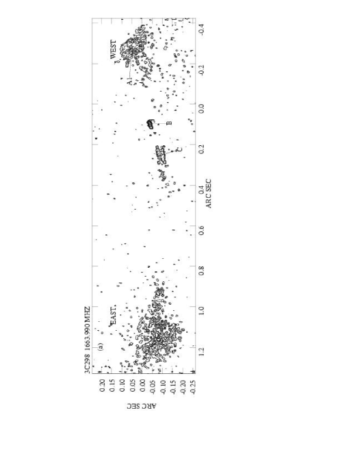
Figure 8: 3C 298 at 8$\times$8 mas (almost full resolution): (a) 18 cm image; contours: (-4.0, $2.0\times 2^{n},n\geq 0)$mJy/beam; $S_{\rm peak}=$0.156 Jy/beam; (b) 6 cm image; contours: (-2.0, $1.0\times 2^{n},n\geq 0)$mJy/beam; $S_{\rm peak}=$0.168 Jy/beam

Figure 9: 3C 298 “core” region at 11$\times$5 mas (high) resolution; (a) 18 cm image; contours: (-4.0, $2.0\times 2^{n},n\geq 0)$mJy/beam; $S_{\rm peak}=$0.147 Jy/beam; (b) 6 cm image; contours: (-4.0, $2.0\times 2^{n},n\geq 0)$mJy/beam; $S_{\rm peak}=$0.332 Jy/beam

At the intermediate resolution of 26$\times$15 mas (Fig. 7) further extended structure disappears into the noise. A number of features are better delineated and component $B$ begins to show hints of extension. At 18 cm (Fig. 7a) the Eastern lobe is very fragmented and the jet at $E$, now well collimated, can be traced, on colour images (not shown), within the lobe. The intermediate jet ($C+D$) is still present, quite collimated but shorter. A ridge of emission seems to run from the “hot–spot” $F$ to South–West. Of the Western lobe only the bright component $A$, now well resolved, and hints of the plume are still visible. The elongated feature East of $A$, that in Fig. 6a could have been interpreted as the Western jet end, appears now quite wide. Note that $A$ is elongated roughly perpendicular to the jet overall direction. At 6 cm (Fig. 7b) only components $A$, $B$, $C$, $E$ and $F$ are still clearly visible.

Images of the entire source, restored with a circular Gaussian beam of $8\times 8$ mas, are shown in Fig. 8. Here we see the “nucleus” and the start at $B$ of the Eastern jet (near jet), the intermediate jet at $C$ and, at 18 cm only, lobes $WEST$ and $EAST$, although much fragmented. It is interesting to note that the intermediate jet has a sharp edge on its western side at both frequencies (although not easy to see in Fig. 8) roughly perpendicular to the jet axis. This feature could be the result of a transverse shock.

At full resolution ($11\times 5$ mas, images not shown) only the region $B$ to $C$ can be well imaged at both frequencies. The two lobes are almost completely resolved out. In the Western one a quite compact bright “true” hot–spot ($A1$ in Table 6), accounting for $\approx$ 10% of component $A$ flux density, stands out at both frequencies clearly distinct from the surrounding low brightness emission. This hot–spot is barely distinguishable from the rest of the lobe in Fig. 8 due to the compressed angular scale. The “hot–spot” $F$ in the Eastern lobe is completely resolved out at both frequencies.

The nuclear region ($B$) is shown in Fig. 9 at the highest available resolution. At least 3 components, labelled $B1,B2,B3$ from West to East, are visible. The VLBA image by Fey & Charlot (fey (1997)) at 2.3 GHz, is in reasonable agreement with ours at 1.7 GHz, which has a similar resolution. From the images in the 1.7–8.4 GHz range we conclude that $B1$ is most likely the “true” core in the source, since it is the most compact feature and has a convex spectrum peaking between 2.3 and 5 GHz (Sect. 3.2.3). Components $B2$ and $B3$ represent the near jet.

Component parameters are given in Table 6 at both 1.7 (first line) and 5 GHz (second line). Observed parameters of all components (but $B$) are measured on the low resolution images (Fig. 6); parameters of $B1,B2,B3$ and of the hot–spot $A1$ are from the high resolution data. The flux density of the extended structure in the two lobes has been determined by measuring the whole lobe flux density with task TVSTAT (Sect. 3) and by then subtracting the contribution of the bright components $A$ and $F$ respectively. Their sizes have been estimated from the contour plots. For all the other components flux density and beam–deconvolved size were obtained using IMFIT.

Derived physical parameters for all components but $B1$ (which is unresolved and with a convex spectrum) have been computed assuming equipartition conditions and are reported in Table 6. They are computed from the 1.7 GHz data, except for $B2$ where we used the 5 GHz data.

Table 6: Observed and Derived Parameters for 3C 298

comp	S	$\theta_{1}\times\theta_{2}$	d${}_{1}\times$d2	$\alpha_{\rm thin}$	H${}_{\rm eq}\ \$	u${}_{\rm min}\ \ \$	U${}_{\rm eq}\ \ \ \$	$\nu_{\rm to}$
	mJy	mas	pc $\leavevmode\nobreak\ h^{-1}$		mG	erg cm${}^{-3}\leavevmode\nobreak\ h\ \$	1054erg $h^{-2}$	MHz
$A$	1024	57$\times$45	245$\times$193	1.28	4.3	1.8$\times 10^{-6}$	1400	234
	193	39$\times$24
${\dagger}A1$	63	$\mathrel{<\kern-10.00002pt\lower 3.87495pt\hbox{$\sim$}}2$	$\mathrel{<\kern-10.00002pt\lower 3.87495pt\hbox{$\sim$}}9$	0.49	$\mathrel{>\kern-10.00002pt\lower 3.87495pt\hbox{$\sim$}}$15	$\mathrel{>\kern-10.00002pt\lower 3.87495pt\hbox{$\sim$}}$2$\times 10^{-5}$	$\mathrel{<\kern-10.00002pt\lower 3.87495pt\hbox{$\sim$}}$1	$\mathrel{>\kern-10.00002pt\lower 3.87495pt\hbox{$\sim$}}$713
(h.sp)	37	$\mathrel{<\kern-10.00002pt\lower 3.87495pt\hbox{$\sim$}}2$
${\dagger}B1$	254	9$\times$2	26$\times$9	0.82				$\sim$3000
	330	unres
${\dagger}B2$	51	unres		0.80
	29	5$\times$4	21$\times$17		1.0	1$\times 10^{-5}$	5.6	477
${\dagger}B3$	33	9$\times$6	39$\times$26	0.87	5.5	2.8$\times 10^{-6}$	6.4	238
	9
$C$	245	43$\times$14	185$\times$60	0.74	3.4	1.1$\times 10^{-6}$	62	187
	102	41$\times$16
$D$	292	157$\times$58	674$\times$249	1.20	1.8	3.0$\times 10^{-7}$	1100	103
	77	162$\times$28
$E$	183	72$\times$26	309$\times$112	1.50	4.3	1.7$\times 10^{-6}$	590	173
	36	$<85\times 35$
$F$	416	108$\times$32	463$\times$137	0.78	1.9	3.6$\times 10^{-7}$	275	118
	107	54$\times$30
$WEST$	973	$\sim$700$\times$400	(3.0$\times 1.7)\times 10^{3}$	1.50	0.6	0.3$\times 10^{-7}$	3900	75
	87	$\sim$470$\times$320
$EAST$	1810	$\sim$800$\times$400	(3.4$\times 1.7)\times 10^{3}$	1.03	0.6	0.6$\times 10^{-7}$	4400	70
	346	$\sim$830$\times$470

1st line: 18 cm data; 2nd line: 6 cm data

${\dagger}$ data from the high resolution image; flux density of $A1$ included in $A$

$\alpha_{\rm thin}$ spectral index in the frequency range 0.3–5 GHz ; H_eq equipartition magnetic field; u_min minimum energy density; U_eq minimum energy; $\nu_{\rm to}$ computed turnover frequency (except for $B1$ which is observed; Sect. 3.2.3)

3.2.2 Jet brightness distribution

In the Eastern jet (near and intermediate portions) we have analyzed the surface brightness $B(\phi)$ at 1.7 GHz as a function of the (beam–deconvolved) jet transverse size ($\phi$) measuring the HPW of the jet perpendicular to its direction at several positions spaced by about one beam, in such a way as to have independent measurements.

The average jet opening angle is $\approx 17^{\circ}$. The deconvolved brightness decreases as $B(\phi)\propto\phi^{-m}$ with $m$ in the range $0.5-2$. In spite of the uncertainties, we conclude that the jet appears highly sub–adiabatic.

3.2.3 Spectral Analysis

The overall spectrum of 3C 298, derived from low resolution measurements (Kuhr et al. kuh (1981); Kameno et al. kame (1995); Steppe et al. step (1995), Murgia et al. mur (1999)) is straight and steep ($\alpha=$1.15) from $\approx$90 GHz (or possibly 230 GHz) down to $\approx$80 MHz, where it turns over.

An attempt to analyze the multi–frequency spectra (from 0.3 to 22 GHz) of the individual components has been carried out adopting a “low–resolution approach” (except for $A1$ and subcomponents of $B$ for which we used the data at the maximum available resolution). A complication is that some components are blended at some frequencies and well separated at others, so that the spectral indices, $\alpha_{\rm thin}$ in Table 6, do not always make use of all the six available frequencies (0.3, 0.6, 1.7, 5, 15, 22 GHz, Sect. 3.2.1). In addition, in order to fully exploit the whole frequency range, we have also fitted the spectra of the blends $E+F$ and $B+C+D$. For components $A1,B1,B2,B3$ two to four frequencies, from this paper and from Fey & Charlot (fey (1997)), are available. All components (and blends), except $B1$, have straight spectra in the available frequency range (often down to 0.3 GHz). Component $B1$, instead, has an inverted spectrum with a maximum around 3 GHz and $\alpha_{\rm thick}$ close to 2.5 between 1.7 and 2.3 GHz.

The two lobes $EAST$ and $WEST$ are heavily resolved in the 15 and 22 GHz images of van Breugel et al. (vanb (1992)) as well as at the low frequencies of 0.6 and 0.3 GHz. Therefore the spectral indices in Table 6 are computed using only the present flux densities at 1.7 and 5 GHz.

As done in Sect. 3.1.2 we computed the source subtracted spectrum by subtraction of the (core $+$ jet) flux densities (components $B+C\&D$) from the overall spectrum. This is a good estimate of the global spectrum of the two lobes (“hot–spots” included) and of the eventually missed low surface brightness features. This spectrum shows a break at $\approx$ 1 GHz, with spectral indices $\alpha_{\rm low}\approx 1$ and $\alpha_{\rm high}\approx 1.6$ respectively below and above it.

4 Discussion

4.1 Sources’ Morphology

In spite of the similarity in radio power the two sources are very dissimilar in radio morphology. 3C 298 has the typical FRII characteristics of a quasar: well separated lobes with “hot–spots”, a one sided jet and a bright core. Most of the radio emission at $\nu\leq 2$ GHz is from the lobes and the “hot–spots”.

On the other hand, 3C 43 has its radio emission dominated by a one-sided jet with sharp bends. Morphologies like these are seen among CSSs (see Mantovani et al. manto (1998) for a collection of similar objects), although they are not the majority. No bright features such as hot–spots are seen in the outer broad components. The overall structure is then far from an FRII type.

4.2 Relativistic Effects and Source Orientation

The presence of relativistic effects in the core and jets of the sources are evaluated by analyzing the core dominance and the jet asymmetry.

The core dominance at 5 GHz is the ratio $R_{\rm c}=S_{\rm c}/S_{\rm ext}$ of the $k-$corrected flux density in the core to that in the extended features. We assume that what we call “core” is actually the sum of the advancing and of the receding bases of the jet, moving on both sides of the true core at the same speed ($\pm\beta_{\rm c}$) and at the same angle ($\theta_{\rm c}$) to the line of sight. The value found for $R_{\rm c}$ is then compared with the median value $\left<R_{\rm c}\right>=$0.05$\pm$0.03 (error is 2$\sigma$) found at 5 GHz by Fanti et al. (fan3 (1990)) for CSS quasars of similar radio luminosity. $\left<R_{\rm c}\right>$ is related to the median angle that quasars make to the line of sight ($\left<\theta\right>\approx 30^{\circ}$ in the unified scheme, Urry & Padovani, urry (1995)). From the “normalized core power” defined as $P_{\rm c,n}=R_{\rm c}/\left<R_{\rm c}\right>\approx\left[(1-\beta{\rm{}_{c}}\leavevmode\nobreak\ \cos\left<\theta\right>)/(1-\beta_{\rm c}\leavevmode\nobreak\ \cos\theta_{\rm c})\right]^{(2+\alpha_{\rm c})}$ (Giovannini et al. giov (1994)) one can estimate ($\beta_{\rm c}\leavevmode\nobreak\ \cos\theta_{\rm c}$). Note that in the calculations we have ignored the contribution of the receding jet, since it is negligible, and have used $\alpha_{\rm c}=0$ to be consistent with Fanti et al. (fan3 (1990)).

The jet/counter–jet brightness ratio is given by:

$R_{\rm j}=\left(\frac{\displaystyle{{1+\beta_{\rm j}\cos\theta_{\rm j}}}}{\displaystyle{{1-\beta_{\rm j}\cos\theta_{\rm j}}}}\right)^{2+\alpha_{\rm j}}$

where $\beta_{\rm j}$ and $\theta_{\rm j}$ are the jet and counter–jet speed and the angle to the line of sight (both assumed to be identical for the two sides of the source) and $\alpha_{\rm j}$ the jet average spectral index. The most appropriate images for this purpose would be those at 1.7 GHz, which however do not show any obvious counter–jet.

Core Dominance

The two sources are quite different in core dominance, since we find:

$\leavevmode\nobreak\ \leavevmode\nobreak\ \leavevmode\nobreak\ \leavevmode\nobreak\ \leavevmode\nobreak\ \leavevmode\nobreak\ \leavevmode\nobreak\ R_{\rm c}=0.012\leavevmode\nobreak\ \leavevmode\nobreak\ \leavevmode\nobreak\ \leavevmode\nobreak\ \leavevmode\nobreak\ P_{\rm c,n}=0.24^{+0.35}_{-0.9}\leavevmode\nobreak\ \leavevmode\nobreak\ {\rm for}\leavevmode\nobreak\ \leavevmode\nobreak\ \leavevmode\nobreak\ 3{\rm C}\leavevmode\nobreak\ 43$

$\leavevmode\nobreak\ \leavevmode\nobreak\ \leavevmode\nobreak\ \leavevmode\nobreak\ \leavevmode\nobreak\ \leavevmode\nobreak\ \leavevmode\nobreak\ R_{\rm c}=0.103\leavevmode\nobreak\ \leavevmode\nobreak\ \leavevmode\nobreak\ \leavevmode\nobreak\ \leavevmode\nobreak\ P_{\rm c,n}=2.1^{+3.1}_{-0.8}\leavevmode\nobreak\ \leavevmode\nobreak\ \leavevmode\nobreak\ \leavevmode\nobreak\ \leavevmode\nobreak\ {\rm for}\leavevmode\nobreak\ \leavevmode\nobreak\ \leavevmode\nobreak\ 3{\rm C}\leavevmode\nobreak\ 298$

(errors are 2 $\sigma$ and are mainly due to the uncertainty in $\left<R_{\rm c}\right>$).

If we assume, according to the unified scheme, that quasar jets are oriented closer than $\approx 45^{\circ}$ to the line of sight, the ranges of the possible angles and $\beta_{\rm c}$ become:

$35^{\circ}\mathrel{<\kern-10.00002pt\lower 3.87495pt\hbox{$\sim$}}\theta_{\rm c}\mathrel{<\kern-10.00002pt\lower 3.87495pt\hbox{$\sim$}}45^{\circ}\leavevmode\nobreak\ \leavevmode\nobreak\ \leavevmode\nobreak\ \leavevmode\nobreak\ \beta_{\rm c}\mathrel{>\kern-10.00002pt\lower 3.87495pt\hbox{$\sim$}}0.75\leavevmode\nobreak\ \leavevmode\nobreak\ \leavevmode\nobreak\ \leavevmode\nobreak\ \leavevmode\nobreak\$ for 3C 43

$\leavevmode\nobreak\ \leavevmode\nobreak\ \leavevmode\nobreak\ \leavevmode\nobreak\ \leavevmode\nobreak\ \leavevmode\nobreak\ \leavevmode\nobreak\ \leavevmode\nobreak\ \leavevmode\nobreak\ \theta_{\rm c}\mathrel{<\kern-10.00002pt\lower 3.87495pt\hbox{$\sim$}}30^{\circ}\leavevmode\nobreak\ \leavevmode\nobreak\ \leavevmode\nobreak\ \beta_{\rm c}\mathrel{>\kern-10.00002pt\lower 3.87495pt\hbox{$\sim$}}0.7\leavevmode\nobreak\ \leavevmode\nobreak\ \leavevmode\nobreak\ \leavevmode\nobreak\ \leavevmode\nobreak\ \leavevmode\nobreak\ \leavevmode\nobreak\$ for 3C 298

Jet/counter–jet ratio

In neither source do we detect the counter-jet, so that we can only set upper limits. To be conservative and to minimize the effects of individual bright knots, we used the average surface brightness on the jet side and twice the local average r.m.s. noise, as upper limit, for the undetected counter–jet. We find:

$\leavevmode\nobreak\ \leavevmode\nobreak\ \leavevmode\nobreak\ \leavevmode\nobreak\ \leavevmode\nobreak\ \leavevmode\nobreak\ R_{\rm j}\mathrel{>\kern-10.00002pt\lower 3.87495pt\hbox{$\sim$}}15\leavevmode\nobreak\ \leavevmode\nobreak\ \leavevmode\nobreak\ \leavevmode\nobreak\ \leavevmode\nobreak\ \leavevmode\nobreak\ \leavevmode\nobreak\ \leavevmode\nobreak\ \leavevmode\nobreak\$ for 3C 43   —–$>\beta_{\rm j}\leavevmode\nobreak\ \cos\theta_{\rm j}\mathrel{>\kern-10.00002pt\lower 3.87495pt\hbox{$\sim$}}0.46$

$\leavevmode\nobreak\ \leavevmode\nobreak\ \leavevmode\nobreak\ \leavevmode\nobreak\ \leavevmode\nobreak\ \leavevmode\nobreak\ \leavevmode\nobreak\ \leavevmode\nobreak\ \leavevmode\nobreak\ \leavevmode\nobreak\ \mathrel{>\kern-10.00002pt\lower 3.87495pt\hbox{$\sim$}}5\leavevmode\nobreak\ \leavevmode\nobreak\ \leavevmode\nobreak\ \leavevmode\nobreak\ \leavevmode\nobreak\ \leavevmode\nobreak\ \leavevmode\nobreak\ \leavevmode\nobreak\ \leavevmode\nobreak\ \leavevmode\nobreak\$ for 3C 298 —–$>\beta_{\rm j}\leavevmode\nobreak\ \cos\theta_{\rm j}\mathrel{>\kern-10.00002pt\lower 3.87495pt\hbox{$\sim$}}0.3$

The above limits do not constrain the jet orientation and speed any better than the core dominance. We note however that for the jet of 3C 43 lower speeds and smaller angles to the line of sight than derived from the core dominance would be permitted, but this would imply a change in the jet direction out of the core $A$ (see also Sect. 4.3).

4.3 Distortions

3C 43 appears as a very distorted radio source, with sharp bends: $\approx 40^{\circ}$ at $C2,\leavevmode\nobreak\ \approx 60^{\circ}$ at $D$ ($\approx$200 mas, i.e. $\approx$850 pc$\leavevmode\nobreak\ h^{-1}$), $\approx 30^{\circ}$ at $F$ (see Figs. 1b and 2). Note that all these sharp bends appear to occur where a bright knot of emission is seen, suggestive of jet–ISM interactions.

On the basis of the present knowledge of NLR properties, Mantovani et al. (manto (1998)) estimated that in up to 10% of CSSs the jets are likely to hit a dense cloud which deflects them without disruption. The physics of jet-cloud interaction has been investigated by de Young (dey (1991)) and Norman & Balsara (norm (1993)) in 3-D hydrodynamical simulations. They show that a jet may maintain its collimation for deflections up to 90^∘. So the distortions we see may well be due to jet interactions with inhomogeneities of the ambient medium.

Sharp deflections might also be due to projection effects on a moderately distorted jet seen close to the line of sight. But this does not seem to be the case for 3C 43. According to Eq. (1) in the Appendix, the large bends we see could only be produced by projection effects if the bright jet is oriented at a very small angle to the line of sight (see also the extended discussion in Conway & Murphy con (1993)). This however is somewhat in contradiction with the discussion of Sect. 4.2, where, from the relative weakness of the core, angles larger than $\sim 30^{\circ}$ were suggested which are too large to produce large apparent deflections. For instance, for $\theta\approx 30^{\circ}$, an observed bend $\zeta\leavevmode\nobreak\ ^{\prime}\sim 95^{\circ}$ is obtained only with an intrinsic bend $\zeta\mathrel{>\kern-10.00002pt\lower 3.87495pt\hbox{$\sim$}}40^{\circ}$. Of course we cannot exclude that the mini-jet within $A$ (Sect. 3.1.1) be at large angles to the line of sight (as deduced from the core dominance), and that it changes its orientation at component $B$. The bright and faint jet (Fig. 2) would then be an intrinsically almost straight jet, oriented close to the line of sight (in agreement with the lack of a counter–jet, Sect. 4.2), whose visible bend is due solely to projection effects. But this would represent again a large intrinsic distortion occurring between $A$ and $B$. So it seems to us not very plausible that all the large bends we see are amplifications of small ones.

We note, finally, that all the bends are always in the same sense, as, e.g., in 3C 119 (Nan et al. 1991a ) and in 3C 287 (Fanti et al. fan2 (1989)). Therefore it appears unlikely that they are just due to random strikes of the jet against several dense NL clouds. A mechanism which governs on which side the jet has to turn around seems to be required (see discussion in Nan et al. 1991a ). An alternative possibility is that we are seeing a helical jet in projection (Conway & Murphy con (1993)), but this seems implausible since this model applies to high $\gamma$ core dominated objects, while 3C 43 it is not.

3C 298 has a much more linear structure, compared to 3C 43. Figs. 6 to 8 show a gentle regular bending. “Hot–spot” $A$ is in p.a.$\approx$$-73^{\circ}$ with respect to $B$. The Eastern jet starts with p.a.$\approx$$120^{\circ}$ and is roughly aligned with the intermediate jet (Fig. 8) then it deviates northward by $\approx$$20^{\circ}$ at about 350 mas (or 1.5 kpc $\leavevmode\nobreak\ h^{-1}$). Since in this case the jet is plausibly oriented at small angles to the line of sight, it is likely that a small intrinsic bending is amplified to the observed value by projection effects.

4.4 Source Ages

A conventional way to estimate a source age, with all the necessary caveats, is via its radiative age. To do so we estimated for both sources the radiation loss frequency break, $\nu_{\rm break}$, in the subtracted spectrum (Sect. 3.1.2 and 3.2.3), which we consider a good approximation of the overall spectrum of the more extended, and hence plausibly older, components, visible or not in the present observations. As pointed out by Murgia et al. (mur (1999)), radiative ages are likely to represent the source age only when the lobes, which have accumulated the electrons produced over the source lifetime, dominate the source spectrum, as it is the case for 3C 43 and 3C 298.

Both subtracted spectra may be fitted by a Continuum Injection model. From $\nu_{\rm break}$ the spectral age has been estimated adopting the equipartition magnetic field (H_eq). Such ages have been compared, whenever possible, with estimates obtained with different methods.

In 3C 43 the $\nu_{\rm break}$ in the subtracted spectrum falls in the range $\approx 0.3$ GHz to $\mathrel{<\kern-10.00002pt\lower 3.87495pt\hbox{$\sim$}}0.1$ GHz, depending on the low frequency behaviour of spectrum of the “Central” component. For an estimated equipartition magnetic field H${}_{\rm eq}\approx 0.5$ mG, the radiative age of the extended components is in the range 2 to 3 $\times 10^{5}$ years.

In the case of 3C 298 the subtracted spectrum has $\nu_{\rm break}\approx 1$ GHz. This implies, for the estimated equipartition magnetic field H${}_{\rm eq}\approx 0.6$ mG, a radiative age $\tau_{\rm r}\approx 7\leavevmode\nobreak\ 10^{4}$y for the extended components.

The age estimates for both sources disagree somewhat with those derived by Murgia et al. (mur (1999)). This is just due to the different frequency breaks adopted by those authors for the total spectrum, which is affected by the presence of the compact structures, and to the equipartition magnetic fields, poorly estimated due to the lack, at that time, of high resolution images.

For 3C 43, which is very twisted and with no visible “hot–spots” (Sect. 4.1), we have no other way to estimate its age. For 3C 298 instead, we have two alternative approaches.

(a) – We noticed earlier that the “jetted lobe” is significantly farther from the core than the “un-jetted” one. This is expected if the heads of the lobes advance at a velocity ($\beta_{\rm h}$) high enough that there are different travel time delays for the radiation from them. The more distant lobe would be the one advancing towards the observer. This is confirmed by the asymmetry in the polarization of the two lobes (Akujor & Garrington, aku3 (1995)), if the latter is interpreted in terms of the “Laing–Garrington” effect (Laing, lai (1988); Garrington et al. garr (1988)). The observed arm ratio is $R_{\rm arm}\approx 2.7:1$. On the assumption that the arm asymmetry is solely due to travel time delays, one obtains a $\beta_{\rm h}\cos\theta\approx 0.45$. For any $\theta\mathrel{<\kern-10.00002pt\lower 3.87495pt\hbox{$\sim$}}30^{\circ}$ (as in the core, Sect. 4.2) we have $\beta_{\rm h}\approx 0.45-0.5$. The above value of $\beta_{\rm h}\cos\theta$ would imply a luminosity ratio of the two “hot–spot” $R_{\rm h.sp.}=R_{\rm arm}^{3+\alpha}\approx 40$, while the observed $R_{\rm h.sp}.$ is $\approx 2.4$ only, and reversed, the supposedly receding “hot–spot” being more luminous than the approaching one. Part of the discrepancy may be attributed to the fact that the receding “hot–spot” $A$ is seen at an earlier stage of evolution compared to the advancing one $F$, which may have suffered radiative/adiabatic losses, but this is not sufficient. We could also speculate that the western arm is shortened by projection if the source structure is not linear but more bent toward the line of sight on the Western side, or that the “hot–spot” luminosities are dominated by relativistic back–flows. However, if we ignore these contradictions and assume that the lobe arm asymmetry is due to travel time delay, we deduce a lower limit for the “kinematic age” of the advancing and of the receding lobes of $\approx 3.2\times 10^{4}\times(\tan\theta)^{-1}$ years and $\approx 1.1\times 10^{4}\times(\tan\theta)^{-1}$ years respectively, which, for $\theta\leq 30^{\circ}$, are very close to the radiative age estimate.

(b) – We can estimate of the source age from energy budget arguments. The equipartition pressure in the “hot–spots” ($p_{\rm h.sp.}$) allows us to compute the jet thrust defined as $\Pi\approx p_{\rm h.sp.}\times{\cal A}$, where ${\cal A}$ is the jet impact area (estimated from the “hot–spot” diameters), and the jet energy flux is defined as $F_{\rm e,j}=c\leavevmode\nobreak\ \Pi$. The time required to feed the lobes (feeding age) is then derived from the ratio $2\times U_{\rm lobe}/F_{\rm e,j}$, where $U_{\rm lobe}$ is the lobe ($EAST$ or $WEST$) minimum total energy and the factor 2 roughly accounts for the work spent to expand the lobe. We obtain feeding ages $\tau_{\rm f}\approx 2-5\times 10^{4}$ years for $WEST$ and $EAST$ respectively, in fair agreement with the previous estimates.

4.5 The external medium

Some inferences on the properties of the medium surrounding the two sources can be obtained from their physical parameters. In the case of 3C 298, taking the source growth velocity derived from the arm ratio in Sect. 4.4, the balance between the ram pressure and the “hot–spot” pressure allows us to estimate the external medium density. We obtain $n_{\rm e}\approx 1\times 10^{-3}$ cm^-3 for “hot–spot” $A$ and a value two times lower for “hot–spot” $F$. Such a density estimate is quite low with respect to others found in the literature (see e.g. O’Dea, ode (1998) and references therein).

Taken at face value, these figures would indicate a decrease of the density with the distance $r$ from the core as $n_{\rm e}\propto r^{-0.7}$, suggesting, from the value of the exponent of $r$, that the lobes are just crossing the gas core radius. The internal pressure of the lobes, coupled to the above density estimate, is incompatible with a static confinement even for very high gas temperatures. It is therefore very likely that the lobes are over-pressured and therefore that they are expanding supersonically.

As pointed out in Sect. 4.1, 3C 43 lacks “hot–spots”. We remark, however, that its broad components have internal pressures not too far from those of the lobes of 3C 298. We are tempted to assume that the external medium properties and dynamics of expansion of the broad components are similar in the two sources. However the medium has to be very clumpy in this source, if the bends are caused by jet-cloud interaction. Furthermore a special space distribution of the clouds is required, in order to act as the wall of a cavity (see Nan et al. 1991a ) and to cause the jet to bend always in the same sense.

5 Summary and conclusions

In this paper we have presented multi–frequency and multi–resolution observations of two CSS quasars from the 3CR catalogue: 3C 43 and 3C 298.

The two sources have similar redshift and radio power, but appear very different in their properties. 3C 298 has all the characteristics of a small FRII radio source. It shows a moderately bright radio core, a one-sided jet and lobes with “hot–spots”. It is likely oriented at $20^{\circ}-30^{\circ}$ to the line of sight but its deprojected linear size is still $\leq 20$ kpc$\leavevmode\nobreak\ h^{-1}$. Its radio luminosity at $\nu\leq 2$ GHz is largely provided by lobes and “hot–spots”.

3C 43 is an object hard to interpret. It is dominated by a knotty jet showing several large bends which cannot be explained by projection effects if the overall source orientation is $\mathrel{>\kern-10.00002pt\lower 3.87495pt\hbox{$\sim$}}30^{\circ}$, as deduced from the weakness of its core. In order to bring the core weakness in agreement with the large distortions being due to projection, one should assume that the jet changes its orientation just out of the core. This would also explain, via Doppler de–boosting, the fact that no counter-jet is seen, in spite of the core weakness. But again, if the jet turns toward the observer just outside the core, this may represent a large intrinsic deflection. We are led to interpret 3C 43 as a radio source intrinsically distorted by jet–cloud interactions. The external medium has to be clumpier than average, in order to cause several large bends, and has to have a very special space distribution to produce the overall clock-wise distortion of the source.

The equipartition magnetic fields are in the range 2–5 mG in most components, reaching several tens of mG in the cores and sub–mG values in the lobes, in agreement with Fanti et al. (fan5 (1995)).

The estimated radiative ages of the extended components of $\approx$2 10⁵ years for 3C 43 and of $\approx 7\times 10^{4}$ years for 3C 298 suggest that these two quasars are moderately young. The radiative age of 3C298 is supported by other arguments based on energy budget considerations and on the arm ratio of the two lobes. The growth velocity of 3C 298 is probably $\approx 0.5c$. The density of the external medium is estimated to be $\approx 10^{-3}$ cm^-3.

We have no such additional arguments for 3C 43.

Appendix A Effect of projection on jet bends

For convenience of the reader we summarize here the geometry of jet projection (see also Moore et al. moor (1981), Conway & Murphy con (1993)). Consider the right–handed coordinate system of Fig. 10 with $Z$ along the line of sight and $XY$ in the plane of the sky. Suppose for simplicity that the jet is made of just two straight segments: $Jet_{1}$ in the plane $ZX$ and at an angle $\theta$ to the line of sight ($Z$), $Jet_{2}$ at an angle $\zeta$ with respect to $Jet_{1}$ ($\zeta=0^{\circ}$ no bending, $\zeta=180^{\circ}$ the jet turns completely backward). The locus of the possible positions in space of $Jet_{2}$ is the surface of a cone with axis $Jet_{1}$ and half opening angle $\zeta$. The position of $Jet_{2}$ on the conical surface is then identified by the azimuthal angle $\phi$ such that for $\phi=0^{\circ}$ or $\phi=180^{\circ}$ $Jet_{2}$ lies in the plane $ZX$ and for $\phi=\pm 90^{\circ}$ $Jet_{2}$ is parallel to $Y$.

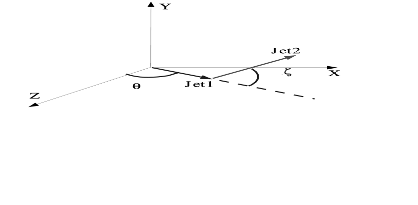
Figure 10: Scheme for jet projection. $Z$ is along the line of sight; $XY$ is the plane of the sky

The relation between the apparent ($\zeta\leavevmode\nobreak\ ^{\prime}$) and the intrinsic ($\zeta$) bending angle is:

$$\tan\zeta\leavevmode\nobreak\ ^{\prime}=\frac{\sin\zeta\sin\phi}{\cos\zeta\sin\theta+\sin\zeta\cos\theta\cos\phi}$$ (1)

It is clear from this equation that certain combinations of $\theta$ and $\phi$ could produce $\zeta\leavevmode\nobreak\ ^{\prime}\approx 90^{\circ}$, even for small $\zeta$. For instance for $\phi=90^{\circ}$ $\zeta\leavevmode\nobreak\ ^{\prime}\rightarrow 90^{\circ}$ when $\theta\rightarrow 0^{\circ}$, independent of $\zeta\not=0$.

References

- (1) Axon, D.J., Capetti, A., Fanti R., et al. 2000, AJ, 120, 2284
- (2) Akujor, C.E., Spencer, R.E., Saikia, & D.J. 1991a, A&A, 249, 337
- (3) Akujor, C.C, Spencer, R.E., Zhang, F.J., et al. 1991b, MNRAS, 250, 215
- (4) Akujor, C.E., & Garrington S.Y. 1995, A&AS 112, 235
- (5) Conway, J.E., & Murphy, D.W. 1993, Ap.J. 411, 89
- (6) Conway, J.E., & Schilizzi, R.T. 2000, 5th European VLBI Network Symposium, J.E. Conway, A.G. Polatidis, R.S. Booth and Y. Pihlström eds. Published by Onsala Space Observatory, p. 123
- (7) de Young, D.S. 1991, Ap.J., 371, 69
- (8) Dallacasa, D., Cai Zhengdong, Schilizzi, R.T., et al. 1994, in Proceedings of the workshop on Compact Extragalactic Radio Sources (Socorro), J.A. Zensus and K.I. Kellermann eds., p.23
- (9) de Vries, W.H., O’Dea, C. P., Baum, S. A., & Barthel, P. D. 1999, ApJ, 526, 27
- (10) Fanti, C., Fanti, R., Parma, P. et al. 1985, A&A, 143, 292
- (11) Fanti, C., Fanti, R., Parma, P. et al. 1989, A&A, 217, 44
- (12) Fanti, R., Fanti, C., Schilizzi, R.T., et al. 1990a, A&A, 231, 333
- (13) Fanti, C., Fanti, R., Dallacasa, D. et al. 1995, A&A, 302, 317
- (14) Fanti, C. 2000, 5th European VLBI Network Symposium, J.E. Conway, A.G. Polatidis, R.S. Booth and Y. Pihlström eds. Published by Onsala Space Observatory, p. 73
- (15) Fey, A.L. & Charlot, P. 1997, ApJS 111, 95
- (16) Garrington, S.T., Leahy, J.P., Conway, R.G., & Laing, R.A. 1988, Nature, 331, 147
- (17) Giovannini, G., Feretti, L., Venturi, T. et al. 1994, ApJ., 435, 115
- (18) Graham, D.A., & Matvejenko, L.I., 1984, IAU Symp. n.110, R. Fanti, K. Kellermann, G. Setti eds., Reidel p. 43
- (19) Kameno, S., Inoue, M., Matsumoto, K. et al. 1995, PASJ, 47,711
- (20) Kuhr, H., Witzel, A., Pauliny–Toth, I.I.K. et al., 1981 A&AS 45, 367
- (21) Laing, R.A. 1988, Nature, 331, 149
- (22) Lüdke, E., Spencer, R.E., Akujor, C.C. et al. 1998, MNRAS, 299, 467
- (23) Mantovani, F., Junor, W., Bondi, M., et al. 1998 A&A 332, 10
- (24) Moore, P.K., Browne, I.W.A., Daintree, E.J., et al. 1981 MNRAS, 197, 325
- (25) Morganti, R., Osterloo, T., Tadhunter, C.N., et al. 2001, MNRAS 323, 331
- (26) Murgia, M., Fanti, C., Fanti, R. et al. 1999, A&A 345, 769
- (27) Nan, R., Schilizzi, R.T., van Breugel, W.J.M, et al. 1991a, A&A, 245, 449
- (28) Nan, R., Schilizzi, R.T., Fanti, C., et al. 1991b, A&A, 252, 513
- (29) Norman, M.L. & Balsara, D.S., 1993, Jets in Extragalactic Radio Sources, eds. K. Meisenheimer &H.J. Rose, Springer Verlag, berlin, p. 229
- (30) O’Dea, C.P. & Stefi, A.B. 1997, AJ, 113, 148
- (31) O’Dea, C. P. 1998, PASP, 110, 493
- (32) Pacholczyk, J.A., 1970, Radio Astrophysics, Freeman, San Francisco
- (33) Pearson, T.J., Perley, R.A., & Readhead, A.C.S., 1985, A.J., 328, 114
- (34) Readhead, A.C.S., Taylor, G.B., Pearson, T.J., & Wilkinson, P.N., 1996, ApJ., 460, 634
- (35) Saikia, D.J., 1988, in Active Galactic Nuclei, Miller H. R. , Wiita P. J., eds, Springer–Verlag, Berlin, p. 317
- (36) Steppe, H., Jeyakumar, S., Saikia, D.J., & Salter, C.J., 1995 A&AS 113, 409
- (37) Spencer, R.E., McDowell, J.C., Charlsworth, M. et al.1989, MNRAS, 240, 657
- (38) Spencer, R.E., Schilizzi, R.T., Fanti, C. et al. 1991. MNRAS, 250, 225
- (39) Urry, C. Megan & Padovani, P. 1995, PASP, 107, 803
- (40) van Breugel, W.J.M., Fanti, C., Fanti, R. et al. 1992, A&A, 256, 56