The Physical Conditions of Intermediate Redshift Mg ii Absorbing Clouds from Voigt Profile Analysis

Abstract

We present a detailed and statistical analysis of the column densities and Doppler $b$ parameters of Mgii absorbing clouds at redshifts $0.4\leq z\leq 1.2$. We draw upon the HIRES/Keck data ($\Delta v\simeq 6.6$ km s^-1) and Voigt profile (VP) fitting results presented by Churchill & Vogt (Paper I). The sample is comprised of 175 clouds from 23 systems along 18 quasar lines of sight. In order to better understand whether the inferred physical conditions in the absorbing clouds could be “false” conditions, which can arise due to the non–uniqueness inherent in parameterizing complex absorption profiles, we performed extensive simulations of the VP analyses presented in this paper. In brief, we find: (1) The Feii and Mgii column densities are correlated at the 9 $\sigma$ level. There is a 5 $\sigma$ anti–correlation between the Mgi/Mgii column density ratio and the Mgii column density. (2) Power–law fits to the column density distributions for Mgii, Feii, and Mgi yielded power–law slopes of $\simeq-1.6,-1.7$, and $-2.0$, respectively. (3) The observed peaks of the Doppler parameter distributions were $\sim 5$ km s^-1 for Mgii and Feii and $\sim 7$ km s^-1 for Mgi. The clouds are consistent with being thermally broadened, with temperatures in the 30–40,000 K range. (4) A two–component Gaussian model to the velocity two–point correlation function (TPCF) yielded velocity dispersions of $54$ km s^-1 and $166$ km s^-1. The narrow component has roughly twice the amplitude of the broader component. The width and amplitude of the broader component decreases as equivalent width increases. (5) From photoionization models we find that the column density ratios are most consistent with being photoionized by the ultraviolet extragalactic ionizing background, as opposed to stellar radiation. Based upon the Mgi to Mgii column density ratios, it appears that at least two–phase ionization models are required to explain the data.

1 Introduction

In Churchill & Vogt (2001, hereafter Paper I), we presented 23 Mgii absorption systems observed at high–resolution in high signal–to–noise quasar spectra. The analysis presented in Paper I was primarily based upon direct measurements of the data. In this paper we concentrate on measurements obtained using Voigt profile fitting of the data.

Voigt profile analysis provides a well defined, if simplistic, parameterization of complex absorption lines. From the beginning of the last decade (e.g., Carswell et al., 1991), Voigt profile (VP) analysis has been a useful technique for statistically documenting the physical conditions of absorbing gas in quasar spectra. VP analysis yields the number of “clouds” in a given absorption complex, their Doppler parameters, and their relative line–of–sight velocities. Since the atomic physics is incorporated, the line–of–sight integrated column densities and the thermal and/or turbulent properties of the gas clouds can be measured.

The reported statistics of both the high redshift Ly$\alpha$ forest (Hu et al., 1995; Lu et al., 1996) and Civ absorbers (Rauch et al., 1996) have been based upon VP decomposition of high resolution ($R\simeq 45,000$) and signal–to–noise ratio ($S/N\simeq 30-80$) spectra. A primary assumption of VP analysis is that complex absorption profiles can be decomposed into a product of individual components, each of which are treated as spatially isolated, isothermal clouds intercepting the incoming flux at a unique line–of–sight velocity. However, numerical simulations of the Ly$\alpha$ forest and of Civ systems at high redshift undermine this physical picture because the absorbing systems merge continuously into a smoothly fluctuating background, often are comprised of a range of temperatures, and are usually broadened by coherent velocity flows (Haehnelt, Stienmetz, & Rauch, 1996; Davé et al., 1997). This is not altogether surprising for higher redshifts, given that Ly$\alpha$ and Civ absorption likely arise in large, coherent structures that are still coupled to the Hubble flow (e.g., Rauch, Haehnelt, & Steinmetz, 1997).

Unblended absorption lines arising in lower ionization gas, as traced by the Mgii $\lambda\lambda 2796,2803$ doublet, are often relatively narrow and suggestive of quiescent single “clouds” (Churchill et al., 1999; Churchill & Charlton, 1999; Churchill & Vogt, 2001). As such, the low ionization gas more directly associated with the components of galaxies may be a better match to the assumptions underlying VP analysis. However, Mgii systems also show a wide variation in kinematic complexity, including significant blending of the profiles arising from the discrete clouds (Petitjean & Bergeron, 1990; Churchill & Vogt, 2001). It is not clear how this particular type of blending could systematically skew the statistical results yielded by VP analysis. In addition, an unavoidable consequence of VP analysis is that the results are sensitive to both the resolution and signal–to–noise ratio of the spectra (Churchill, 1997; Rauch et al., 2002).

Even with the many caveats mentioned above, the potential for VP analyses to answer many questions regarding the physical nature of the absorbing gas remains widely recognized. What is the average number of clouds per system? What is the distribution of column densities and column density ratios? How does the cloud–cloud velocity clustering depend upon equivalent width? Are the line broadening mechanisms thermal, or dominated by turbulent motions in the gas? With the aid of state of the art photoionization models we can ask: What are the chemical and ionization conditions of the studied ionic species? What can be inferred about the nature of the ionizing radiation? If there is a stellar contribution, what limits can be placed on the numbers of stars and their distances from the gas clouds?

For Mgii systems, answers to some of these questions have been investigated using data with a resolution of $~{}30$ km s^-1 (Petitjean & Bergeron, 1990; Bergeron et al., 1994). Since VP analysis is strongly dependent upon spectral resolution, it is a logical step to re–examine the statistical distributions previously inferred for Mgii systems with higher resolution data. In this paper we present statistical results from a VP analysis of an ensemble of 23 Mgii–selected absorbers obtained with the HIRES instrument (Vogt et al., 1994) on the Keck I telescope. The resolution of these data is $\simeq 6$ km s^-1. The systems and the VP results were previously presented in Paper I.

In § 2, we briefly review the data. In § 3, we describe the VP analysis of the data, our VP decomposition methodology, and simulations of the analysis for purposes of diagnosing whether or not a given statistical result is induced, in part or in full, by the VP technique itself. In § 4, we present the distribution of VP column densities, Doppler parameters, and velocities. We also provide some analysis of these distributions. Photoionization models of the VP components, or clouds, are discussed in § 5. We include an exploration of the possible relative contribution of stellar flux to that of a standard ultraviolet background. We outline the main results of this paper in § 6.

2 The Data

The acquisition, calibration, and analysis of the data has been described in Churchill (1997) and in Paper I. However, we provide a brief description here. We emphasize that all systems are selected by the presence of Mgii $\lambda\lambda 2796,2803$ absorption.

The quasar spectra were obtained with the HIRES instrument (Vogt et al., 1994) on the Keck I telescope. The spectral resolution is $R=45,000$. The signal–to–noise ratio in the continuum near the Mgii absorption profiles is typically $\sim 30$. A total of 23 systems comprise the sample of absorbers. The sample includes only those systems with Mgii $\lambda 2796$ rest–frame equivalent width, $W_{r}(2796)$, greater than $0.3$ Å. The ensemble of systems is considered to be representative of a “fair”, or unbiased sample, in that the distribution of Mgii equivalent widths is consistent with that of unbiased surveys (e.g., Lanzetta, Turnshek, & Wolfe, 1987; Steidel & Sargent, 1992; Churchill et al., 1999).

The sample has been divided into four subsamples by their equivalent widths. Sample B has $W_{r}=(0.3,0.6]$ Å, sample C has $W_{r}=(0.6,1.0]$ Å, sample D has $W_{r}\geq 0.6$ Å, and sample E has $W_{r}\geq 1.0$ Å. We have used the notation “(” to denote inclusive and “]” to denote exclusive. These samples are historically motivated (see Steidel & Sargent, 1992). In Table 1 we present the systems by quasar, absorber redshift, and sample membership. Also listed is a system identification, or ID.

The Mgii $\lambda 2796$ profiles are presented in Figure 1. The spectra are normalized and converted to rest–frame velocity. The systems are grouped by sample membership and are ordered by increasing $W_{r}$. The system ID and equivalent width are given in each panel. Each system has been modeled using Voigt profile (VP) analysis, as described in Paper I. The solid curves through the data are the VP model spectra and the ticks above the spectra are the VP centroids.

3 Voigt Profile Analysis

We used the Voigt profile fitting program MINFIT (Churchill, 1997) to obtain a least–squares fit (LSF), $\chi^{2}$ minimized model of each absorption line profile. MINFIT sets up M nonlinear functions in N parameters and drives the NETLIB slatec LSF routine DNLS1 (More, 1978; Hiebert, 1980). The N parameters are the redshifts, column densities, and Doppler $b$ parameters for each VP component. The MINFIT program statistically minimizes the number of VP components used to model a given system. Numerical convergence is set to the machine precision of a Sun Ultra 1. Further details are provided in Churchill (1997).

As discussed in Paper I, we concentrate our analysis on the Mgii $\lambda\lambda 2796,2803$ doublet, the Mgi $\lambda 2852$ transition, and the Feii $\lambda 2344$ $2374$, $2582$, $2587$, and $2600$ multiplet. The atomic data used for the VP analysis are given in Table 2 of Paper I. The column densities, $b$ parameters, and cloud velocities output by MINFIT are given in Table 7 of Paper I and illustrated for all transitions in Figure 2 of Paper I.

The resulting VP model spectra for the Mgii $\lambda 2796$ transitions are shown in Figure 1 as solid curves through the data. Ticks above the spectra give the number of VP components and their rest–frame velocities. In Figure 2, we show a detail of the fit for both members of the Mgii doublet for system S15. For this system, seven individual VP components (dotted curves) successfully model the complex profile shape. For the illustrated velocity region, the reduced chi–square was $\chi^{2}_{\nu}=1.3$ for $418$ degrees of freedom (including one Mgi and five Feii transitions each with 50–60 pixels).

Since VP analysis yields a non–unique interpretation of complex absorption lines, it is important to outline key specifics of the fitting procedure and calibration of the results if the analysis is to be considered objective. In the following, we briefly outline the fitting methodology applied in this work, with focus on specifics of the operations performed by the MINFIT code. We also describe simulations of VP analysis that we use to calibrate our statistical results.

3.1 Profile Fitting Methodology

3.1.1 The Number of VP Components

MINFIT employs significance testing in order to return the minimum number of VP components. Two user–defined, run–time parameters, $f_{err}$ and $f_{c}$, provide the maximum fractional error allowed in a VP component and the confidence level at which a VP component is considered statistically significant, respectively. These parameters are adjustable, which adds a subjective element to an otherwise objective, well defined algorithm. Typical values for $f_{err}$ and $f_{c}$ are 1.5 and 0.97, respectively.

Once a LSF solution is obtained, MINFIT computes errors in the standard fashion using the diagonal elements of the covariance matrix, which are obtained from the inversion of the curvature matrix. The elements of the curvature matrix are computed as described in Churchill (1997).

The fractional error of each VP component is the quadrature sum of the fractional errors in the three VP parameters, $N$, $b$, and $z$. When the fractional error of a component exceeds $f_{err}$, the component is dropped. The LSF and error computations are iterated until no components have fractional errors exceeding $f_{err}$.

At this stage the significance level is determined for the VP component with the largest fractional error. The target VP component is dropped and a new LSF solution is obtained. Then, an $F$–distribution test is performed between the two LSF solutions. If the VP component was significant with a confidence level of $f_{c}$ or better, than the original LSF model is restored. If not, the statistical significance is determined for the VP component with the largest fractional error in the new model. This process is repeated until all VP components are significant at a minimum confidence level of $f_{c}$.

3.1.2 Redshifts

It was assumed that the redshifts, $z$, and therefore rest–frame velocities, of each VP component are aligned for all ions. VP components were defined by the presence of Mgii absorption features even if there were no Feii or Mgi absorption features at the same velocity.

We note that the ionization potential of Mgi is below the hydrogen edge. The adopted methodology of enforcing an aligned velocity for all ions may not be sound if the gas has an ionization structure that correlates with line of sight velocity. That is, Mgi could, in principle, arise from a physically and/or kinematically distinct part of the clouds in comparison to Mgii and Feii.

3.1.3 Column Densities

For each VP component, the column densities, $N$, of different ions are determined independent of one another. When multiple transitions of a given ion are available, then the increased number of constraints yield a more robust measurement. For Mgi there is only the singlet. For Mgii there is always the resonance doublet and for Feii there are often three to five transitions of the multiplet available. As such, Mgi is the least constrained ion.

If neither Mgi nor Feii had detectable absorption at the same velocity as a Mgii component, then an upper limit on the Mgi or Feii column density is quoted for the component. This limit is taken from the 3 $\sigma$ equivalent width threshold for an unresolved absorption line at the expected location of the component (see Churchill et al., 2000a).

3.1.4 Doppler Parameters

The line broadening, or $b$ parameter, of a VP component can be written as the convolution of a thermal component and a turbulent component. In order to preserve the Voigt profile formalism, one is required, perhaps quite unrealistically, to parameterize the turbulence with a Gaussian distribution, yielding $b^{2}=b_{therm}^{2}+b_{turb}^{2}$. Whereas $b_{therm}$ scales with the inverse square root of the ion mass, $b_{turb}$ is independent of ion mass and will have the same magnitude for all ions.

There are three possible treatments of the $b$ parameters. In each VP component, one can: (1) measure the $b$ parameter independently for each ion with no assumptions about thermal scaling or level of turbulence, (2) force the $b$ parameter to be equal for all ions, which holds if the turbulent component dominated, or (3) force the turbulent component to be some fraction of the measured $b$ parameter (zero for pure thermal). We assume the first approach, so that we can fully explore the line broadening mechanism.

3.2 Calibrating Our VP Analysis

The only way to calibrate VP analysis is to quantify the degree to which the fitted parameters reflect the “true” cloud properties in cases where they are known a priori. This requires simulations for which the VP parameters obtained from analysis of synthetic spectra can be directly compared to the VP parameters used to generate these spectra.

We have run a series of comprehensive simulations of Mgii absorbers for varying degrees of line blending (i.e. complexity of absorption profiles) and for a range of spectral signal–to noise ratios (i.e. equivalent width detection threshold) commensurate with the data. These simulations have been described in detail in Churchill (1997), and serve to quantify any possible bias, systematic, or random errors in the VP results to the data. For each analysis using VP fits to the observational data, we performed an identical analysis using VP fits to the synthetic spectra. In this way, the systematics or significance of any observational statistical result can be quantified and any systematic skew in the functional form of a distribution can be estimated.

The simulations required input column density, $b$ parameter, and velocity clustering distributions. We used the data to guide our “best” choices of these distribution functions by comparing (1) the distribution of pixel flux decrements, (2) the distribution of equivalent widths of the kinematic subsystems, (3) the distribution of velocity widths of the kinematic subsystems, and (4) the observed VP component column density, $b$ parameter, and velocity distributions.

The adopted distributions for the simulations were obtained by constructing a set of 500 simulated absorption systems and performing VP analysis on these spectra. We then performed statistical tests comparing the simulation distributions and the observed distributions to eliminate those which were not statistically consistent with data (also see Charlton & Churchill, 1998). For the Mgii column densities, we chose a power law distribution, $f(N)\propto N^{-\delta}$ with $\delta=1.6$. The $b$ parameters distribution was drawn from a Gaussian with centroid $4$ km s^-1, a width of $\sigma=1.5$ km s^-1 and a lower cut–off of $1.5$ km s^-1. The lower cut off was required to match the small $b$ portion of the observed distribution. For the VP component velocity clustering, we chose a Gaussian distribution with $\sigma=45$ km s^-1.

We also simulated the Feii multiplet. We enforced thermal broadening for all VP components, i.e. the $b$ parameters scaled as $b({\hbox{{\rm Fe}\kern 1.00006pt{\sc ii}}})=\{m({\rm Mg})/m({\rm Fe})\}^{1/2}b({\hbox{{\rm Mg}\kern 1.00006pt{\sc ii}}})$, where $m$ is the atomic mass. We also assumed a linear relationship between $\log N({\hbox{{\rm Fe}\kern 1.00006pt{\sc ii}}})$ and $\log N({\hbox{{\rm Mg}\kern 1.00006pt{\sc ii}}})$ for all components. This relation, $\log N({\hbox{{\rm Fe}\kern 1.00006pt{\sc ii}}})=\log N({\hbox{{\rm Mg}\kern 1.00006pt{\sc ii}}})-0.3$, is based upon preliminary VP fitting to the sample presented in Churchill (1997).

Similar simulations for VP analysis calibration have been undertaken by Lu et al. (1996) and by Hu et al. (1995) for the Ly$\alpha$ forest. The significant difference between the simulation performed here and those for the Ly$\alpha$ forest are that (1) the hydrogen absorption–selected clouds were assumed to be distributed cosmologically, whereas the Mgii absorbing clouds are clustered in kinematic systems, and (2) the VP analysis of the Mgii systems included simultaneous fitting to the Mgii doublet and Feii multiplet.

4 Results of Voigt Profile Analysis

4.1 Number of VP Components (i.e. Clouds)

In Figure 3$a$ we show the distribution of the number of VP components (i.e. clouds). The dotted–line histogram represents the full sample of 23 systems. The shaded histogram represents a subset of the full sample in which the very large $N({\hbox{{\rm H}\kern 1.00006pt{\sc i}}})$ systems (S2, S5, and S7) have been removed. These damped Ly$\alpha$ absorbers (DLAs) and “Hi–rich” systems (Churchill et al., 2000b) have been removed in light of their characteristic black–bottomed Mgii absorption profile morphologies; it is difficult to constrain the number of clouds in these systems (they are systematically underestimated unless there are good constraints from weak Feii transitions). For ease of discussion, we will refer to this subset of our 23 systems as the “non–DLA” subset.

For both the full sample and the non–DLA subset, there is an average of 7.7 clouds per absorber. The mode of the binned distribution is eight clouds. In the simulations of complex, blended profiles, $\sim 30$% of the inputted VP components were not recovered. These simulations also revealed that the percentage of unrecovered components decreases with decreasing signal–to–noise ratio, but that the width of the recovered distribution becomes larger as the signal–to–noise ratio increases. To the extent that VP components (such as those in our models) give rise to the observed absorption profiles, the distribution plotted in Figure 3$a$ would require a correction such that the average and mode is elevated to 10–11 clouds per system.

In Figure 3$b$, we show the rest–frame equivalent width of Mgii $\lambda 2796$ versus the number of VP components, $N_{cl}$. The unfilled data points are the DLA and Hi–rich systems. As has been reported previously (Petitjean & Bergeron, 1990; Churchill et al., 1996; Churchill, 1997), there is a very strong correlation between the equivalent width and the number of VP components. A linear LSF, including errors in the equivalent widths, was performed on the data presented in Figure 3$b$. The dotted line is the fit to the full sample, which yielded a slope of $0.058\pm 0.004$ Å/cloud and an equivalent width of $0.28\pm 0.03$ Å for $N_{cl}=1$ (the intercept at $N_{cl}=0$ has no physical meaning).

A fit to the non–DLA subset yielded a statistically identical slope with a slightly smaller value of $0.23\pm 0.03$ Å for $N_{cl}=1$. This fit is shown as the solid line on Figure 3$b$. Thus, at least in this sample of 23 systems, the three DLA and Hi–rich systems serve only to slightly increase the intercept to the fit and do not skew the slope. We also examined whether the data point at $N_{cl}=18$ was dominating the fit results by removing it and refitting to the non–DLA subset of data; the resulting fit was statistically identical to the fit to the full sample.

The slopes of the linear relationship presented here are slightly smaller than both the slopes of $0.070\pm 0.004$ Å/cloud reported by Churchill et al. (1996) for a smaller sample of 15 systems and $0.076\pm 0.004$ Å/cloud reported by Churchill (1997) for a sample of 36 systems. This difference is most likely due to the fact that in this work we did not enforce the fit to pass through the origin, whereas the fit was forced through the origin in the previous work. We stress that the slope is strongly dependent upon the spectral resolution of the data. For example, Petitjean & Bergeron (1990) obtained a much steeper slope of $0.35$ Å/cloud for a large sample observed at a resolution of $\simeq 30$ km s^-1.

4.2 Column Densities

In Figure 4, we present Feii and Mgi column densities vs.  Mgii column densities. Only components for which the errors are less than 0.7 dex are plotted. Upper limits on the Feii and Mgi column densities are shown as open points with downward pointing arrows and measured values are shown as solid points with $1~{}\sigma$ error bars.

$N(\hbox{\hbox{{\rm Fe}\kern 1.00006pt{\sc ii}}})$ is strongly correlated with $N(\hbox{\hbox{{\rm Mg}\kern 1.00006pt{\sc ii}}})$. A Spearman–Kendall test yields a $9~{}\sigma$ significance. Assuming a linear relationship of the form $\log N({\rm X})=a\log N({\hbox{{\rm Mg}\kern 1.00006pt{\sc ii}}})+b$, we determined the best fit parameters using a $\chi^{2}$ minimization that allowed for errors in the Feii, Mgi, and Mgii column densities. The best fit parameters are $a=0.73\pm 0.06$ and $b=3.0\pm 0.8$ for Feii and $a=0.45\pm 0.05$ and $b=5.2\pm 0.6$ for Mgi. Limits have been included in the fitting.

The reduced $\chi^{2}$ is $30$ for Feii and is $27$ for Mgi. Fits to the Feii vs. Mgii and Mgi vs. Mgii column densities obtained from the simulations yielded $\chi^{2}\simeq 10$. Thus, the variance in the data is roughly a factor of three greater than the variance due to statistical scatter inherent in the VP fitting.

In Figure 5, we present Feii to Mgii and Mgi to Mgii column density ratios vs. Mgii column densities. The data presented are the same VP components shown in Figures 4$a$ and 4$b$. Upper limits on the ratios are shown as open points with downward pointing arrows and measured values are shown as solid points. The error bars are suppressed, but they are effectively identical to those presented in Figure 4.

The distribution of $N({\hbox{{\rm Fe}\kern 1.00006pt{\sc ii}}})/N({\hbox{{\rm Mg}\kern 1.00006pt{\sc ii}}})$ visually appears to be a slightly decreasing function of $N({\hbox{{\rm Mg}\kern 1.00006pt{\sc ii}}})$, but is statistically consistent with no dependence upon $N({\hbox{{\rm Mg}\kern 1.00006pt{\sc ii}}})$. This would indicate that $N({\hbox{{\rm Fe}\kern 1.00006pt{\sc ii}}})/N({\hbox{{\rm Mg}\kern 1.00006pt{\sc ii}}})$ is fairly independent of or only slightly decreasing with increasing $N({\hbox{{\rm Mg}\kern 1.00006pt{\sc ii}}})$. The greater than 1 dex spread in the ratio would indicate a range of [$\alpha$/Fe] abundance patterns, dust depletion factors, ionization conditions, or a combination of all three.

There is a significant ($5~{}\sigma$) anti–correlation between $N({\hbox{{\rm Mg}\kern 1.00006pt{\sc i}}})/N({\hbox{{\rm Mg}\kern 1.00006pt{\sc ii}}})$ and $N({\hbox{{\rm Mg}\kern 1.00006pt{\sc ii}}})$ over a 2.5 order of magnitude range of the ratio. For the upper limits, taken by themselves, this trend is an artifact of the limiting detectable $N({\hbox{{\rm Mg}\kern 1.00006pt{\sc i}}})$, which is effectively a constant independent of $N({\hbox{{\rm Mg}\kern 1.00006pt{\sc ii}}})$. However, for the measured ratios, the anti–correlation is real and cannot easily be explained as an artifact of the VP analysis of the data. A linear LSF to the detections only (filled data points of lower panel in Figure 5) yielded a slope of $a=-0.73\pm 0.06$ and intercept $b=7.6\pm 0.3$. The linear fit and its uncertainty are superimposed on the data.

Further discussion of the column density ratios is presented in § 5 in the context of photoionization models.

4.3 Column Density Distribution

VP analysis of simulated spectra with comparable signal–to–noise ratios revealed that the input column density distribution is recovered within the $1~{}\sigma$ errors when an appropriate lower–limit, cut–off column density is applied to a maximum likelihood fit. This cut off is the column density below which the detection completeness drops rapidly.

The simulations further revealed that the completeness level is sensitive to the kinematic clustering of components due to line blending. In regions of significant blending the 90% completeness levels are $\log N({\hbox{{\rm Mg}\kern 1.00006pt{\sc ii}}})=12.4$ cm^-2 and $\log N({\hbox{{\rm Fe}\kern 1.00006pt{\sc ii}}})=12.2$ cm^-2 (we did not examine blending effects for Mgi). The 90% completeness levels for unblended lines are $\log N({\hbox{{\rm Mg}\kern 1.00006pt{\sc ii}}})=11.6$ cm^-2, $\log N({\hbox{{\rm Fe}\kern 1.00006pt{\sc ii}}})=11.8$ cm^-2, and $\log N({\hbox{{\rm Mg}\kern 1.00006pt{\sc i}}})=11.4$ cm^-2. Thus, there is a column density range of “partial completeness”, a transition from incompleteness due to line blending to incompleteness due to finite signal-to–noise ratio.

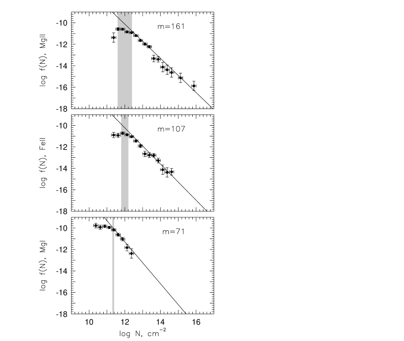
Figure 6: The logarithmic VP column density distribution functions for Mgii (top), Feii (center), and Mgi (bottom). The maximum likelihood results (unbinned data) for the relation $f(N)\propto N^{-\delta}$ are $\delta=1.59\pm 0.05$, $1.69\pm 0.07$, and $2.02\pm 0.03$ for Mgii, Feii, and Mgi, respectively. The number of clouds, $m$, in each sample is written in each panel. The shaded areas show the column density ranges where line blending leads to “partial completeness” (see text).

In Figure 6, the column density distribution functions are shown for Mgii, Feii, and Mgi. The data are binned for purpose of presentation. The shaded regions show the column density ranges of partial completeness. The data appear to follow a power–law distribution, with the turnover at small column densities due to incompleteness. At HIRES/Keck resolution, an unresolved Mgii line saturates at $\log N\simeq 13.5$ cm^-2 and this explains the increased scatter in the number density of Mgii VP components with column densities greater than this value (see Figure 4.3 of Churchill, 1997).

For the column density distribution, we assumed a power law

$$f(N)=CN^{-\delta},$$ (1)

where $f(N)$ is the number of clouds with column density $N$ per unit column density. The total number of clouds, $m$, normalizes $f(N)$ over the observed data according to

$$\int_{N_{\rm min}}^{N_{\rm max}}f(\hat{N})d\hat{N}=m.$$ (2)

We used the maximum likelihood method (e.g., Tytler et al., 1987; Lanzetta, Turnshek, & Wolfe, 1987) to obtain the power–law slope and normalization. The method is performed on the unbinned data. In Figure 6, the solid lines through the data are the maximum likelihood solutions, which are

$${\hbox{{\rm Mg}\kern 1.00006pt{\sc ii}}}:\quad\delta=1.59\pm 0.05\quad C=(9.85\pm 0.16)\times 10^{8},$$ (3)

$${\hbox{{\rm Fe}\kern 1.00006pt{\sc ii}}}:\quad\delta=1.69\pm 0.07\quad C=(1.01\pm 0.22)\times 10^{10},$$ (4)

$${\hbox{{\rm Mg}\kern 1.00006pt{\sc i}}}:\quad\delta=2.02\pm 0.28\quad C=(6.21\pm 0.79)\times 10^{12}.$$ (5)

For this analysis, we used the cut–off column densities appropriate for blended lines, which yielded $m=161$, $107$, and $71$ for Mgii, Feii, and Mgi, respectively.

Using the parameterization given in Equation 1, Petitjean & Bergeron (1990) found a $\delta=1.0\pm 0.1$ for Mgii over the range $12.0\leq\log N(\hbox{\hbox{{\rm Mg}\kern 1.00006pt{\sc ii}}})\leq 14.3$ cm^-2. The resolution of their data was $\sim 30$ km s^-1, and it is likely that their best fit slope is affected by unresolved blending. The expected trend is that the number of large column density components would decrease, being redistributed into a greater number of smaller column density components as the resolution is increased. This would result in a steeper slope, as we have found in this work.

The slopes of the Mgii and Feii column density distributions are very similar, and roughly consistent with one another. However, the slope of Mgi distribution is significantly steeper. These findings are consistent with the distribution of column density ratios presented in Figure 5. There is no correlation of $N({\hbox{{\rm Fe}\kern 1.00006pt{\sc ii}}})/N({\hbox{{\rm Mg}\kern 1.00006pt{\sc ii}}})$ with $N({\hbox{{\rm Mg}\kern 1.00006pt{\sc ii}}})$, yet there is a significant anti–correlation of $N({\hbox{{\rm Mg}\kern 1.00006pt{\sc i}}})/N({\hbox{{\rm Mg}\kern 1.00006pt{\sc ii}}})$ with $N({\hbox{{\rm Mg}\kern 1.00006pt{\sc ii}}})$.

4.4 Doppler Parameter Distribution

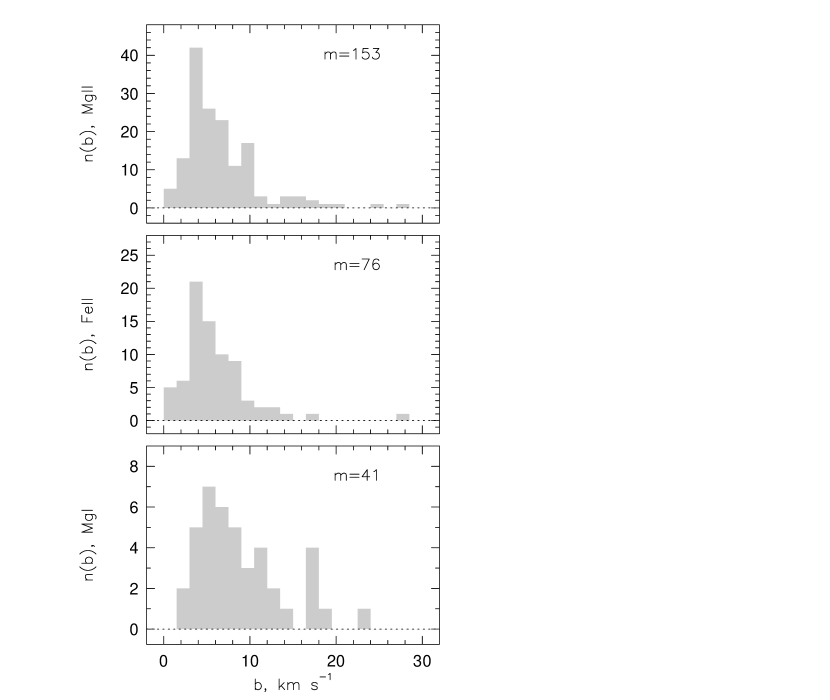
Figure 7: The binned distributions of the VP Doppler $b$ parameters for Mgii (top), Feii (center), and Mgi (bottom). The median Doppler parameters and the standard deviations of the distributions are $\left<b\right>=5.4\pm 4.3$, $5.1\pm 4.1$, and $7.7\pm 5.1$, for Mgii, Feii, and Mgi, respectively. The number of clouds, $m$, in each sample is written in each panel.

The binned distribution of Mgii, Feii, and Mgi Doppler $b$ parameters is presented in Figure 7. The median Doppler parameters and the standard deviations of the distributions are $\left<b\right>=5.4\pm 4.3$, $5.1\pm 4.1$, and $7.7\pm 5.1$, for Mgii, Feii, and Mgi, respectively. We note that, statistically, the relative distributions of Mgii and Mgi are unphysical; it is difficult to understand how Mgi could have broader lines than Mgii on average.

Based upon simulations, the observed distribution peak for Mgii could be shifted to a larger value by $\sim 1$–$2$ km s^-1 compared to the “true” distribution. The true Mgii distribution is likely peaked at $b=3$–$4$ km s^-1. Simulations further indicate that the true distribution may have zero to few clouds with $b\leq 1$ km s^-1. A lower cut–off $b$ parameter of $1.5$ km s^-1 is required to not overproduce the lowest bin. However, we note that this could be a resolution effect, given that lines are unresolved for $b\leq 2.46$ km s^-1.

In $30$ km s^-1 resolution data, Petitjean & Bergeron (1990) measured a Mgii $b$ distribution peaking at $10\leq b\leq 15$ km s^-1, with a decaying tail at $b\geq 20$ km s^-1. They suggest that non–thermal or turbulent motions within the individual clouds are implied because such large $b$ values correspond to temperatures in excess of $10^{5}$ K, a temperature too high for Mgii to survive if photoionized. Our results are suggestive of clouds that are less turbulent and/or cooler, with temperatures between $30$–$40,000$ K. In our data, all VP components with $b>10$ km s^-1 occur in broad, partially or fully saturated profiles.

Simulations revealed that the majority of the large $b$ parameters forming the extended tail to the distribution is an artifact of component blending. Approximately $70$% of the input VP components were recovered; that is, three of ten components were typically lost because of blending. As such, some components may have large $b$ parameters in cases where two components may have been responsible for the absorption profile, but could not be formally constrained by the fitting algorithm.

4.5 Thermal and Turbulence Broadening

The $b$ parameter of a given ion can have both a thermal and non–thermal component. This latter contribution to the line broadening could be due to internal turbulent motion or systematic, bulk motion. Assuming the non–thermal component can be parameterized as a Gaussian distribution preserves the Voigt profile formalism. We note that a Gaussian non–thermal motion in an isolated cloud is difficult to understand, since it implies a mixing, or quasi–convective process that would be expected to decay away in a cloud dynamical time.

The total $b$ parameter of ion $i$ is written,

$$b^{2}_{i}=b^{2}_{i,therm}+b^{2}_{turb},$$ (6)

where $b_{i,therm}=\sqrt{2kT/m_{i}}$ is the thermal component, which scales with the ion mass $m$, and $b_{turb}$ is the non–thermal component, which is equal for all ions. The thermal and non–thermal $b$ parameters for two ions of different mass are determined by solving two equation with two unknowns, which gives

$$b_{turb}=\left[\frac{b^{2}_{j}-(m_{i}/m_{j})b^{2}_{i}}{1-(m_{i}/m_{j})}\right]^{1/2},$$ (7)

and

$$b_{i,therm}=\left[\frac{b^{2}_{i}-b^{2}_{j}}{1-(m_{i}/m_{j})}\right]^{1/2},$$ (8)

where $b_{i}$ and $b_{j}$ are the measured $b$ parameters for the lighter and heavier ions, respectively. This technique for exploring the line broadening mechanism has been applied using Civ and Siiv at $z\sim 2.5$ by Rauch et al. (1996).

In Figure 8, we present the results of deconvolving the thermal and non–thermal components to the line broadening of Mgii and Feii components. The selected data have $b$ parameters with fractional errors less than 50% for both Mgii and Feii. The thermal component is plotted along the vertical and the total $b$ parameter is plotted along the horizontal axis. The solid curves are lines of constant non–thermal motion. The temperature scale for the thermal component is given on the right hand vertical axis.

Clouds that lie above the $b_{turb}=0$ km s^-1 curve have unphysical Mgii to Feii $b$ parameter ratios (recall that the $b$ parameters were fit assuming no constraining relationship between different ions). The mean turbulent component of the subsample is $0.7\pm 0.3$ km s^-1. VP analysis of simulated spectra in which the clouds are assumed to be thermally broadened, i.e. have $b_{turb}=0$ km s^-1, yielded a mean $b_{turb}$ of $\sim 1$ km s^-1. This value is consistent with the value obtained for the data and is suggestive of thermally broadened clouds.

Furthermore, the results from the simulated spectra showed the same level of scatter as the observed data plotted on Figure 8. As such, it is difficult to claim a non–thermal component in individual systems on a case–by–case basis. Based upon the simulations, it is found that the scatter decreases with increasing signal–to–noise ratio. We also note that even though the multiple Feii transitions offer greater constraints on the Feii $b$ parameter, the weaker strength Feii data often have signal–to–noise ratios a factor of $2$–$3$ lower than the Mgii data.

The simulation results and the spread of the data about the $b_{turb}=0$ km s^-1 curve provide no compelling statistical evidence for a non–thermal component to the line broadening of Mgii absorbing gas. From thermal components, the cloud temperatures are inferred to be in the range $30,000$–$150,000$ K. Based upon the photoionization modeling, it is difficult to understand temperatures in excess of $60,000$ K. Again, we note that the clouds with the largest $b$ parameters are due to the blending of components.

4.6 Cloud–Cloud Velocity Clustering

We computed the velocity two–point clustering function (TPCF) for the VP components obtained with our HIRES/Keck spectra (these data are listed in Table 7 of Paper I). As computed here, the TPCF, $P(\Delta v)$, is the probability that any randomly selected pair of VP components in a system will have a velocity splitting $\Delta v$.

Using low resolution spectra, Sargent, Steidel & Boksenberg (1988) used the TPCF to show that Mgii systems clustered on velocity scales of $\Delta v\leq 200$ km s^-1. This was taken as evidence that Mgii systems cluster like field galaxies. Using moderate resolution spectra ($\sim 30$ km s^-1), Petitjean & Bergeron (1990) found that a two component Gaussian model with $\sigma_{1}=80$ and $\sigma_{2}=390$ km s^-1 provided a good fit to the Mgii TPCF. They interpreted the smaller width to reflect the kinematics of clouds bound within galactic halos and the broader width to reflect the kinematics of galaxy pairs in the field.

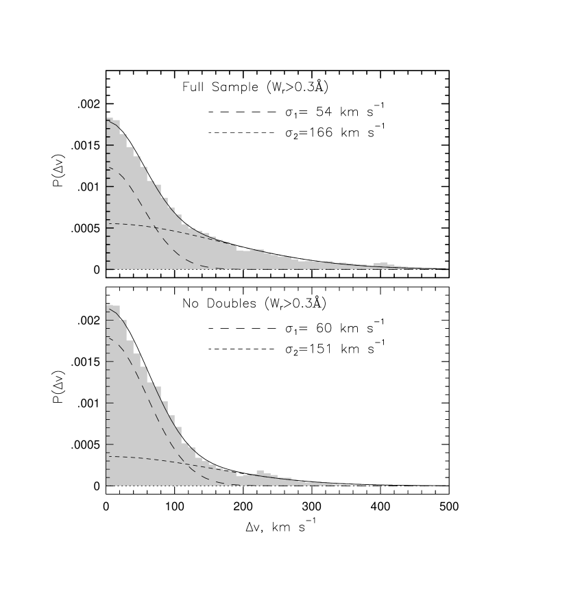
Figure 9: (top) The VP component velocity two–point correlation function (TPCF) for the full sample. The distribution is well described by a double Gaussian function with a narrow dispersion of $\sigma_{1}=54$ km s^-1 and a broader dispersion of $\sigma_{2}=166$ km s^-1. — (bottom) The TPCF for the with double systems removed. The narrow dispersion is $\sigma_{1}=60$ km s^-1 and the broader dispersion is $\sigma_{2}=151$ km s^-1.

The TPCF for the full sample is presented in the upper panel of Figure 9. The TPCF increases sharply for $\Delta v\leq 100$ km s^-1 and has an extended tail out to $\simeq 400$ km s^-1. Following Petitjean & Bergeron (1990), we parameterized the TPCF as a two–component Gaussian,

$$P(\Delta v)=A_{1}\exp\left(\frac{\Delta v^{2}}{2\sigma^{2}_{1}}\right)+A_{2}\exp\left(\frac{\Delta v^{2}}{2\sigma^{2}_{2}}\right),$$ (9)

where the $A$ and $\sigma$ are the amplitudes and Gaussian widths, respectively. We obtained a narrow width of $\sigma_{1}=56$ km s^-1 and a broader width of $\sigma_{2}=166$ km s^-1 for the full sample. The relative amplitudes differ by a factor of two, with the narrow component dominating.

We examined whether the extended tail of the distribution is dominated by the three kinematically complex systems, S1, S9, and S12 (see Figure 1). Not only do these systems have a large kinematic spread, they have roughly twice the Ly$\alpha$ absorption strengths and very strong Civ absorption compared to “classic” Mgii systems; they are classified as “double systems” (Churchill et al., 2000b).

If the double systems are removed from the sample and the TPCF recomputed, we obtain the results presented in the lower panel of Figure 9. For this “No Doubles” sample, we obtained a narrow width of $\sigma_{1}=60$ km s^-1 and a broader width of $\sigma_{2}=151$ km s^-1. The component widths are not substantially different from the full sample TPCF. However, the amplitude of the broad component is a factor of five smaller than that of the narrow component. This indicates that the double systems strongly govern the amplitude of the broad component to the full–sample TPCF, but that the component still results because of “moderate–” and “high velocity” kinematic subsystems in the “classic” Mgii absorbers (Churchill et al., 2000b).

4.7 Evolutionary Clues from Kinematics

It is difficult to apply a straight–forward, physical interpretation to each of the two components of the TPCF. However, based upon absorber models (Churchill, 1997; Charlton & Churchill, 1998), the narrow component width may be proportional to the vertical velocity dispersion of gas in galaxies disks (averaged over random inclination angles). This is also consistent with the notion that the dominant kinematic subsystems (see Paper I), could arise in systematically rotating disks (e.g., Lanzetta & Bowen, 1992; Charlton & Churchill, 1998; Churchill & Vogt, 2001).

The data directly constraining this scenario are few in number; in four out of five edge–on spiral galaxies hosting $W_{r}(2796)\geq 0.3$ Å absorption, the gas kinematics directly trace the outer extensions of the stellar disk rotation curves (Steidel et al., 2002). However, the data are difficult to understand in terms of a simple disk model. Counter examples are also few; Lanzetta et al. (1997) and Ellison, Mallén–Ornelas, & Sawicki (2002) have each reported an example inconsistent with a rotating disk scenario.

Clues to the nature of the broader component to the TPCF might be connected to the redshift evolution of $W_{r}(2796)$. Steidel & Sargent (1992) showed that as the minimum equivalent width of a Mgii–absorber sample is increased, the redshift number density evolution becomes stronger. That is, the strongest systems evolve away most rapidly with decreasing redshift (increasing cosmic time) from $z\simeq 2$ to $z\simeq 0.3$. The underlying physical process governing this evolution remains a mystery, though it has been attributed to either a reduction in the mean column density of the clouds with time (chemical, ionization, and/or gas mass evolution) or a reduction in the velocity spread of the clouds with time (kinematic evolution), or both.

To explore trends in the kinematics with equivalent width, we computed a separate TPCF for samples B, C, D, and E, with and without double systems. The results are listed in Table 2. From these distributions, we see that the nature of the cloud–cloud clustering is strongly connected to the equivalent width.

Including double systems, the velocity dispersion of the narrow component, $\sigma_{1}$, does not change significantly with increasing $W_{r}(2796)$, whereas the broad component velocity dispersion, $\sigma_{2}$, decreases and its relative amplitude, $A_{2}/A_{1}$, increases. If our sample is taken to be representative of the population of Mgii absorbers, this trend in the TPCF would suggest that the frequency of highest velocity clouds decreases as equivalent width is increased (note that the exclusion of the double systems makes no change to the results for sample B.) In other words, in the largest equivalent width systems, the cloud velocities are distributed more uniformly throughout the full velocity interval of the profile and clouds at extreme velocities are less frequent.

Excluding double systems, the extended tail in the TPCF vanishes for samples D and E. Apparently there are two types of kinematics characterizing the very strongest equivalent width systems, and they are extreme to one another. The first type is exemplified by systems S1 and S9 (double systems), where the profile morphology is characterized by a large velocity spread of many clouds representing a wide range of optical depths. Systems S5 and S7 (which are DLAs or near–DLAs) are examples of the second type. The Mgii profile morphology of DLAs and near–DLAs, in the studied redshift regime, are characterized by fully saturated, black–bottom absorption with a moderate kinematic spread of $\sim 60$ km s^-1 (Churchill et al., 2000b).

These findings may provide insight into the nature of the differential equivalent width evolution quantified by Steidel & Sargent (1992). Since the redshift number density of DLAs apparently does not evolve over the redshift range 0.5 to 2.0 (Rao & Turnshek, 2000), those large equivalent width Mgii systems arising in DLAs would also not evolve over this redshift interval. Therefore, if the kinematics of the largest equivalent width systems do fall into the above two categories, and one type arises primarily in DLAs, then it must be the double systems undergoing the most rapid evolution.

This would suggest that Mgii absorption cross section of the kinematically higher velocity material is decreasing with time. However, moderate– and high–velocity kinematic subsystems with weak absorption do not contribute significantly to the total equivalent width in a system. Thus, the evolution cannot be dominated by a decrease in the frequency of weak subsystems in double systems like S1 and S12. It must be an evolution in systems more like S9, where the optical depth is highly variable and relatively large across the entire kinematic range of absorption. At even larger equivalent widths, $\simeq 2$ Å and greater, the evolution is likely dominated by systems with kinematics similar to those studied by Bond et al. (2001). A sample of high resolution Mgii systems at $z>1$ will be required to ultimately address these issues.

4.8 Column Densities and Kinematics

In Figures 10$a$–10$c$, we present the logarithmic column densities for Mgii, Feii, and Mgi. Solid points are measurements and open points are upper limits. The anti-correlations with velocity are induced by the definitions of the velocity zero point. The zero points are defined as the optical depth median of the absorption profiles and virtually all of them are aligned with the centroid of a dominant kinematic subsystem (see Paper I). The dispersion of the column densities decreases with velocity, though it is not clear whether the very small dispersion for $v>200$ km s^-1 is due to small number statistics.

For $\log N({\hbox{{\rm Mg}\kern 1.00006pt{\sc ii}}})\leq 12.5$ cm^-2, the distribution of Mgii column densities is quite flat with velocity, which indicates that low column density clouds are present at all velocities. For these clouds, Feii and Mgi are often below the detection threshold of the data. This explains the presence of upper limits for Feii and Mgi at all velocities, and most obviously at high velocities.

For our sample, we can at least say that it is rare to find large column density clouds at large velocities from the dominant kinematic subsystem (also see Paper I). As trivial as this observation may seem, it has implications for the systematics in the absorption kinematics and therefore possibly the absorber geometry. Apparently, finding two large kinematic subsystems in a single absorber is rare. These subsystems are comprised of several blended components, which is suggestive of gas that is part of a coherent structure with low velocity dispersion, i.e. systematic kinematics. Since there is only a single dominant kinematic subsystem per absorber and if its kinematics are systematic, the geometry is likely to be quasi–planar with velocities primarily parallel to the plane.

In Figures 10$d$ and 10$e$, we present $\log N({\hbox{{\rm Fe}\kern 1.00006pt{\sc ii}}})/N({\hbox{{\rm Mg}\kern 1.00006pt{\sc ii}}})$ and $\log N({\hbox{{\rm Mg}\kern 1.00006pt{\sc i}}})/N({\hbox{{\rm Mg}\kern 1.00006pt{\sc ii}}})$ vs. cloud velocity. Interestingly, the dispersion of $\log N({\hbox{{\rm Fe}\kern 1.00006pt{\sc ii}}})/N({\hbox{{\rm Mg}\kern 1.00006pt{\sc ii}}})$ with velocity is fairly constant with a range from $-1$ to $+0.2$ out to $v\simeq 200$ km s^-1. This would suggest that the range of physical conditions (abundance pattern, dust depletion, ionization conditions) governing this ratio does not change dramatically with kinematics. If, as suggested above, the main kinematic subsystems are single coherent structures, then it may be that the higher velocity clouds are “cloudlettes” surrounding this structure. If so, then these “cloudlettes” apparently do not differ greatly in their Feii to Mgii conditions. Beyond $v\simeq 200$ km s^-1 we can only comment that there are no clouds in our sample with elevated $N({\hbox{{\rm Fe}\kern 1.00006pt{\sc ii}}})/N({\hbox{{\rm Mg}\kern 1.00006pt{\sc ii}}})$.

Since Mgi absorption is present primarily at velocities less than $\simeq 100$ km s^-1, it is less clear if the dispersion of $\log N({\hbox{{\rm Mg}\kern 1.00006pt{\sc i}}})/N({\hbox{{\rm Mg}\kern 1.00006pt{\sc ii}}})$ with velocity is decreasing at larger velocities. In fact, 65% of the detected Mgi arises within $v<30$ km s^-1 and 80% arises with $v<60$ km s^-1. The range of $N({\hbox{{\rm Mg}\kern 1.00006pt{\sc i}}})/N({\hbox{{\rm Mg}\kern 1.00006pt{\sc ii}}})$ for $v<60$ km s^-1, however, is four orders of magnitude (excluding the point at $\log N({\hbox{{\rm Mg}\kern 1.00006pt{\sc i}}})/N({\hbox{{\rm Mg}\kern 1.00006pt{\sc ii}}})=0$). This suggests that the conditions where Mgi arises are probably quite varied. This is likely an ionization condition effect. It could be due to differing cloud densities, ionizing flux, or to multiphase ionization conditions (see next section).

5 Photoionization Models

A grid of Cloudy 90 (Ferland, 1998) photoionization models were constructed in order to place constraints on the chemical and ionization conditions of the VP components. Several researchers have applied photoionization models to Mgii–selected absorption systems (e.g., Bergeron & Stasińska, 1986; Bechtold, Green, & York, 1987; Bergeron et al., 1994; Churchill & Charlton, 1999). A useful exposition on the methods used here has been written by Steidel (1990).

In brief, the clouds are assumed to be plane–parallel, constant density “slabs” with an external ionizing flux incident upon one face of the cloud. For this configuration, the ionization condition is quantified using the ionization parameter, $U=n_{\gamma}/n_{\rm H}$, where $n_{\gamma}$ is the number density of hydrogen ionizing photons and $n_{\rm H}$ is the number density of hydrogen atoms. The quantity $n_{\gamma}$ is dependent upon both the intensity (amplitude at 1 Ryd) and shape of the ionizing spectrum. The clouds are given a pre–defined neutral hydrogen column density, $N({\hbox{{\rm H}\kern 1.00006pt{\sc i}}})$. This results in well–defined clouds that are indexed by their $U$ and $N({\hbox{{\rm H}\kern 1.00006pt{\sc i}}})$ values. We produced a grid of model clouds over the range $-5\leq\log U\leq-1$ and $15\leq\log N({\hbox{{\rm H}\kern 1.00006pt{\sc i}}})\leq 20$ cm^-3 at half dex intervals in both quantities.

In these photoionization models, the column density ratios of various ions are effectively independent of metallicity. Only when metallicity approaches the solar value, resulting in increased cooling rates, are the ratios modified from those in lower metallicity clouds. We use 1/10th solar metallicity ($Z=-1$) for our models. We also use a solar abundance pattern.

5.1 Ionizing Spectrum

The spectral energy distribution (SED) and intensity of the ionizing flux is most uncertain. We explored both an extragalactic ultraviolet background (UVB) source and “local” stellar sources. For the UVB, we used the spectra of Haardt & Madau (1996). These spectra have only slightly different SEDs for $z=1$ and $z=0.5$ with normalizations at 1 Ryd of $\log\nu f_{\nu}=-5.2$ and $-5.6$ erg s^-1 cm^-1, respectively. We find that there is negligible difference in the column density ratios of Feii and Mgi to Mgii for cloud models ionized by these two UVB spectra. For the following discussions, we use the $z=1$ SED.

Assuming no shielding of the UVB, stellar radiation must dominate over the UVB before the stellar SEDs begin to alter column density ratios in cloud models. The ionization potentials to destroy Mgii and Feii are slightly greater than 1 Ryd, whereas the ionization potential to destroy Mgi is slightly below. As shown in Appendix B of Churchill & Le Brun (1998), only O and B stars are capable of modifying the UVB in this energy range for astrophysically reasonable stellar number densities. They also reported that their results were insensitive to stellar surface gravity. Thus, we limited our exploration to stars with $T=30,000$ K, to represent B stars, and with $T=50,000$ K, to represent O stars. Following Churchill & Le Brun (1998), we used the solar metallicity stellar models produced by Kuruzc (1991).

As with the UVB grids, we produced a grid of model clouds over the range $-5\leq\log U\leq-1$ and $15\leq\log N({\hbox{{\rm H}\kern 1.00006pt{\sc i}}})\leq 20$ cm^-3 at half dex intervals in both quantities. We also varied the $\log\nu f_{\nu}$ of stars at 1 Ryd over the range $-7$ to $-3$ erg s^-1 cm^-2 at 1 dex intervals. We produced a separate grid for B and O stars, respectively. For the stellar SEDs, there is a sharp edge at 1 Ryd with a relatively flat energy distribution at energies just greater than 1 Ryd. Thus, for subsequent discussion, we focus on the normalization of the stellar grids at 1.2 Ryd, which is very close to the ionization potentials to destroy Mgii and Feii. For reference, the $z=1$ UVB at 1.2 Ryd has $\log\nu f_{\nu}=-5.3$ erg s^-1 cm^-2.

5.2 Limits on Stars and Their Distances

Following the formalism of Churchill & Le Brun (1998), we derive the minimum number of O, B I, and B V stars in a confined region at a distance of $R$ kiloparsecs, that are required to influence the ionization conditions to be

$$\log N_{\ast}({\rm O})=0.1+2\log R,$$ (10)

$$\log N_{\ast}({\rm B~{}I})=0.0+2\log R,$$ (11)

$$\log N_{\ast}({\rm B~{}V})=0.8+2\log R,$$ (12)

at $z=1$. The constants are reduced by 0.4 for $z=0.5$. These constants were computed using the flux level of the UVB SED at 1.2 Ryd, effectively at the ionization potentials of Mgii and Feii. To recompute $N_{\ast}$ for a known stellar flux, $\nu f_{\nu}$ at 1.2 Ryd, one simply adds $5.3+\log\nu f_{\nu}$.

We have assumed that the photon escape fraction from the stellar environment is 100%. Under the assumption of a grey opacity, $\log N_{\ast}$ would be increased by $|\log f_{esc}|$, where $0<f_{esc}\leq 1$. In Figure 11, we plot $\log N_{\ast}$ vs. $\log R$ for the three stellar types at $z=1$. We apply these results below.

5.3 Feii to Mgii Ratio

In Figure 12, we show results of the photoionization models for the Feii to Mgii column density ratios overplotted on the data. Six panels are shown. The upper left panel shows the SEDs for the assumed ionizing continuum. The thick solid curve is the Haardt & Madau UVB at $z=1$. The thinner solid curves are the SEDs of $T=30,000$ (B–type) stars for flux levels $\log(\nu f_{\nu})=-3.9$ and $-5.2$ erg s^-1 cm ^-2 at 1.2 Ryd. The dashed curves are the SEDs of $T=50,000$ (O–type) stars for flux levels $\log(\nu f_{\nu})=-2.4$ and $-4.4$ erg s^-1 cm ^-2 at 1.2 Ryd. These normalizations were chosen because the lower flux grids illustrate minor modifications and the higher flux grids represent significant modifications to the UVB models. The lower left panel shows the UVB photoionization grid superimposed upon the data. The mostly vertical curves are constant logarithmic neutral hydrogen column density, $\log N({\hbox{{\rm H}\kern 1.00006pt{\sc i}}})$, and the mostly horizontal curves are constant logarithmic ionization parameter, $\log U$. The column density contours start at $\log N({\hbox{{\rm H}\kern 1.00006pt{\sc i}}})=20$ cm^-2 and decrease by 0.5 dex intervals toward the left. The ionization parameter contours start at $\log U=-5$ and increase by 0.5 dex intervals downward. The four remaining panels show the grids for the stellar ionizing continua. The grid contours follow the same pattern.

The UVB model is consistent with a larger majority of the measured $N({\hbox{{\rm Fe}\kern 1.00006pt{\sc ii}}})/N({\hbox{{\rm Mg}\kern 1.00006pt{\sc ii}}})$ ratios. There are, however, several clouds that have measured ratios of $\log N({\hbox{{\rm Fe}\kern 1.00006pt{\sc ii}}})/N({\hbox{{\rm Mg}\kern 1.00006pt{\sc ii}}})>0$ and lie above the model grid. Adjusting the $\alpha$–group to iron–group abundance pattern, [$\alpha$/Fe], in the models is equivalent to “sliding” the model grid parallel to the $N({\hbox{{\rm Fe}\kern 1.00006pt{\sc ii}}})/N({\hbox{{\rm Mg}\kern 1.00006pt{\sc ii}}})$ axis. However, astronomical ratios range from $[\alpha/{\rm Fe}]=0$ (solar) for $-1\leq Z\leq 0$ to $[\alpha/{\rm Fe}]=+0.5$ ($\alpha$ enhancement) for $Z<-1$ (e.g., Lauroesch et al., 1996). The model grid would slide downward 0.5 dex for the $\alpha$ enhancement pattern. Since we assumed a solar pattern for the models the grid cannot be elevated further. Thus, it is not possible to model these these clouds by assuming a standard non–solar [$\alpha$/Fe]. It is also not possible to simply assume a standard dust depletion pattern. In warm interstellar medium clouds, iron depletes more readily than does magnesium; iron and magnesium have depletion factors of $\delta=-1.4$ and $-0.7$, respectively (Lauroesch et al., 1996). Assuming a standard dust depletion would slide the model grid downward, aggravating the problem.

Some of the elevated column density ratios could be an artifact of the VP fitting parameterization. At Keck/HIRES resolution, an unresolved Mgii line saturates (core intensity of zero) at $\log N\simeq 13$ cm^-2. In this regime of $N({\hbox{{\rm Mg}\kern 1.00006pt{\sc ii}}})$, the VP fitting simulations of blended absorption lines yielded roughly 10% by number VP components with similarly elevated $N({\hbox{{\rm Fe}\kern 1.00006pt{\sc ii}}})/N({\hbox{{\rm Mg}\kern 1.00006pt{\sc ii}}})$ ratios. It is thus plausible that a fair fraction of those clouds with $\log N\simeq 13$ cm^-2 have elevated $N({\hbox{{\rm Fe}\kern 1.00006pt{\sc ii}}})/N({\hbox{{\rm Mg}\kern 1.00006pt{\sc ii}}})$ ratios as an artifact of the VP fitting process.

However, this explanation cannot be invoked for those clouds with $\log N({\hbox{{\rm Mg}\kern 1.00006pt{\sc ii}}})<13$ cm^-2. The VP fitting simulations in this regime of $N({\hbox{{\rm Mg}\kern 1.00006pt{\sc ii}}})$ do not yield any components with elevated $N({\hbox{{\rm Fe}\kern 1.00006pt{\sc ii}}})/N({\hbox{{\rm Mg}\kern 1.00006pt{\sc ii}}})$ ratios. Interestingly, in our sample, 15 clouds with $\log N({\hbox{{\rm Mg}\kern 1.00006pt{\sc ii}}})<13$ cm^-2 have $N({\hbox{{\rm Fe}\kern 1.00006pt{\sc ii}}})/N({\hbox{{\rm Mg}\kern 1.00006pt{\sc ii}}})>0$. It is worth noting that the ratios in these clouds hold some similarity to the “iron–rich” weak Mgii systems (Rigby et al., 2000). Though the global environments of the clouds in these strong systems may be very different than those of the weak systems, the physical processes that give rise to their abundance ratios (see discussion in Rigby et al., 2000) may be one and the same local to the clouds.

Using Feii and Mgii as a diagnostic of the presence of stellar flux is not very useful because of the large degeneracy between the column density ratios predicted for the different spectral shapes. The stellar SEDs tend to yield a maximum Feii to Mgii ratio that decreases as the stellar flux is increased. This is especially true for the O stars. It is not ruled out that B stars can be contributing to the stellar flux for many of the model clouds illustrated. For B I stars, there would need to be $\sim 40,000~{}(100,000)$ in number to make a minimum discernible contribution at a distance of $R=10~{}(20)$ kpc from the clouds (see Equation 11 and Figure 11).

5.4 Mgi to Mgii Ratio

In Figure 13, we show results of the photoionization models for the Mgi to Mgii column density ratios overplotted on the data. The photoionization grids are the same as described for the six panels of Figure 12. The Mgi balance is complicated by both a dielectronic recombination process and a charge exchange reaction with Hii. We compared model clouds for which these two mechanisms were included to those for which the mechanisms were “turned off”. In the relatively narrow density regime and temperature regime of the grids, the inclusion or exclusion of these processes did not influence the Mgi to Mgii ionization fraction.

Illustrated in Figure 13 are two major discrepancies between the data and the models.

First, there is no single–phase photoionization model presented that can explain clouds having $\log N({\hbox{{\rm Mg}\kern 1.00006pt{\sc i}}})/N({\hbox{{\rm Mg}\kern 1.00006pt{\sc ii}}})>-1.8$. Though the results presented here are statistical and involve comparing the data to a grid of models, we note that even detailed photoionization modeling involves struggles to reproduce observed Mgi to Mgii column density ratios (Churchill & Charlton, 1999; Ding et al., 2002; Rauch et al., 2002).

Ding et al. (2002) argue that the majority of the Mgi gas arises in a lower temperature ($T\sim 500$ K), virtually non–turbulent, higher density phase than does the bulk of the Mgii absorption. That is, the Doppler $b$ parameters of the Mgi clouds are, in reality, significantly smaller ($b\simeq 1$ km s^-1), than those of the bulk of the Mgii absorption ($b\simeq 5$ km s^-1). If Ding et al. are correct, then “unphysical” observed large column density ratios are an artifact of VP fitting, which does not enforce any physical connection between the Mgi and Mgii gas. In this scenario, much of the Mgii absorption would arise in a separate phase, warmer than that of the Mgi. If so, then the single–phase models presented in Figure 13 do not apply to the a substantial fraction of the Mgi data.

To avoid a high density solution, Rauch et al. (2002) suggest a large $N({\hbox{{\rm Mg}\kern 1.00006pt{\sc i}}})/N({\hbox{{\rm Mg}\kern 1.00006pt{\sc ii}}})$ ratio in the $z=0.5656$ system toward Q$2237+0305$ may indicate a large $N({\hbox{{\rm H}\kern 1.00006pt{\sc i}}})$, on the order of a DLA. This cannot be the case for the majority of the large ratio clouds studied here because (1) it would imply too large a redshift path density for DLAs in this redshift range (Rao & Turnshek, 2000), and (2) only three systems (S2, S5, and S7) are known to have near–DLA or DLA hydrogen column densities (Churchill et al., 2000a, b).

The second discrepancy between the data and the models in Figure 13 is that no model is consistent with the observed anti–correlation between $\log N({\hbox{{\rm Mg}\kern 1.00006pt{\sc i}}})/N({\hbox{{\rm Mg}\kern 1.00006pt{\sc ii}}})$ and $\log N({\hbox{{\rm Mg}\kern 1.00006pt{\sc ii}}})$. This slope is $\Delta\log[N({\hbox{{\rm Mg}\kern 1.00006pt{\sc i}}})/N({\hbox{{\rm Mg}\kern 1.00006pt{\sc ii}}})]/\Delta\log N({\hbox{{\rm Mg}\kern 1.00006pt{\sc ii}}})=-0.73$ over the range $11.5\leq\log N({\hbox{{\rm Mg}\kern 1.00006pt{\sc ii}}})\leq 14.5$ cm^-2.

We searched for other correlations and anti–correlation between the Mgi VP parameters and the Mgii VP parameters to see if the anti–correlation between $\log N({\hbox{{\rm Mg}\kern 1.00006pt{\sc i}}})/N({\hbox{{\rm Mg}\kern 1.00006pt{\sc ii}}})$ and $\log N({\hbox{{\rm Mg}\kern 1.00006pt{\sc ii}}})$ could be induced by systematics in the VP fitting. If $b({\hbox{{\rm Mg}\kern 1.00006pt{\sc i}}})/b({\hbox{{\rm Mg}\kern 1.00006pt{\sc ii}}})>1$ for the majority of the clouds [an unphysical condition unless Mgi is associated with gas more turbulent than is Mgii], and/or if this ratio were found to increase as $N({\hbox{{\rm Mg}\kern 1.00006pt{\sc ii}}})$ increases, this could induce the observed anti–correlation. However, accounting for uncertainties, all $b({\hbox{{\rm Mg}\kern 1.00006pt{\sc i}}})/b({\hbox{{\rm Mg}\kern 1.00006pt{\sc ii}}})$ are consistent with unity and there is no correlation between $b({\hbox{{\rm Mg}\kern 1.00006pt{\sc i}}})/b({\hbox{{\rm Mg}\kern 1.00006pt{\sc ii}}})$ and $N({\hbox{{\rm Mg}\kern 1.00006pt{\sc ii}}})$. There is also no correlation between $b({\hbox{{\rm Mg}\kern 1.00006pt{\sc i}}})/b({\hbox{{\rm Mg}\kern 1.00006pt{\sc ii}}})$ and $N({\hbox{{\rm Mg}\kern 1.00006pt{\sc i}}})/N({\hbox{{\rm Mg}\kern 1.00006pt{\sc ii}}})$. As such, there appears to be no obvious VP fitting correlation that is inducing the observed anti–correlation between $\log N({\hbox{{\rm Mg}\kern 1.00006pt{\sc i}}})/N({\hbox{{\rm Mg}\kern 1.00006pt{\sc ii}}})$ and $\log N({\hbox{{\rm Mg}\kern 1.00006pt{\sc ii}}})$.

Interestingly, the curves of constant ionization parameter for the highest $\log\nu f_{\nu}$ stellar models run parallel to the slope, $\Delta\log[N({\hbox{{\rm Mg}\kern 1.00006pt{\sc i}}})/N({\hbox{{\rm Mg}\kern 1.00006pt{\sc ii}}})]/\Delta\log N({\hbox{{\rm Mg}\kern 1.00006pt{\sc ii}}})$, but they underpredict the Mgi to Mgii column density ratio by roughly 1 dex. Also note, however, that the stellar fluxes for the illustrated models require an unreasonable number of ionizing stars; at a distance of 20 kpc, roughly $4\times 10^{5}$ O stars and roughly $2\times 10^{6}$ B I stars are required.

On the other hand, if the metallicity of the model clouds were increased about 1.5 dex, which would effectively move the photoionization grids directly to the right on the panels in Figure 13, then the model ratios could be consistent with the clouds having $\log N({\hbox{{\rm Mg}\kern 1.00006pt{\sc ii}}})\geq 13.5$ cm^-2. However, models of the lower Mgii column density clouds could not be made consistent with the data. We also note that the required metallicity would be 0.5 dex greater than solar (this argument is independent of abundance pattern).

There appear to be two real discrepancies between the observation and single–phase ionization models: (1) single–phase models are not consistent with $\log N({\hbox{{\rm Mg}\kern 1.00006pt{\sc i}}})/N({\hbox{{\rm Mg}\kern 1.00006pt{\sc ii}}})>-1.8$; and (2) the models cannot explain the observed anti–correlation between $\log N({\hbox{{\rm Mg}\kern 1.00006pt{\sc i}}})/N({\hbox{{\rm Mg}\kern 1.00006pt{\sc ii}}})$ and $\log N({\hbox{{\rm Mg}\kern 1.00006pt{\sc ii}}})$. As Ding et al. (2002) point out for two–phase models, each phase can have $\log N({\hbox{{\rm Mg}\kern 1.00006pt{\sc i}}})/N({\hbox{{\rm Mg}\kern 1.00006pt{\sc ii}}})<-1.8$ while the combined absorption from these two phases can be made consistent with the total observed absorption strengths (equivalent widths) of Mgi and Mgii, respectively. Further exploration of the phenomenological and physical conditions governing the Mgi to Mgii absorption strengths is beyond the scope of this paper and is planned for future study.

6 Conclusions

We have performed an analysis on the Voigt profile fitting results reported by Churchill & Vogt (2001) for 23 Mgii–selected quasar absorption line systems. The quasar spectra were observed with the HIRES instrument (Vogt et al., 1994) on the Keck I telescope and have a velocity resolution of $\sim 6$ km s^-1. For most of the Mgii systems, several Feii transitions and the Mgi $\lambda 2852$ transition were available for study. Further details on the data and the Voigt profile fitting have been presnted by Churchill (1997) and Churchill & Vogt (2001).

In general, we have examined both the statistical properties of the number of components, and the component column densities, Doppler parameters, and velocities. Where appropriate, we have compared our findings with identical analyses on simulated data in order to ascertain possible statistical bias or systematics. These simulation results have provided insights into the degree to which an observational result is or is not an artifact of the Voigt profile fitting formalism. Further details of the simulations can be found in Churchill (1997).

The statistical results of the VP analysis are summarized as follows:

(1) The Feii and Mgii column densities are correlated at the 9 $\sigma$ level. A least–squares linear fit yielded $\log N({\hbox{{\rm Fe}\kern 1.00006pt{\sc ii}}})=0.73\log N({\hbox{{\rm Mg}\kern 1.00006pt{\sc ii}}})+3.0$. A fit to the Mgi column densities yielded $\log N({\hbox{{\rm Mg}\kern 1.00006pt{\sc i}}})=0.45\log N({\hbox{{\rm Mg}\kern 1.00006pt{\sc ii}}})+5.2$. There is a 5 $\sigma$ anti–correlation of the Mgi column density with the ratio of the Mgi to Mgii column densities.

(2) The column density distributions for Mgii, Feii, and Mgi were parameterized with a power–law of the form $f(N)\propto N^{-\delta}$. The maximum likelihood power–law indices were found to be $\delta\simeq 1.6,1.7$, and $2.0$, respectively. Within 1 $\sigma$ uncertainties, the Feii and Mgii column density indices are consistent with one another. However, the Mgi index is significantly steeper than those for Feii and Mgii. There is a 5 $\sigma$ anti–correlation between the ratio $N({\hbox{{\rm Mg}\kern 1.00006pt{\sc i}}})/N({\hbox{{\rm Mg}\kern 1.00006pt{\sc ii}}})$ and $N({\hbox{{\rm Mg}\kern 1.00006pt{\sc ii}}})$ which follows $\log N({\hbox{{\rm Mg}\kern 1.00006pt{\sc i}}})/N({\hbox{{\rm Mg}\kern 1.00006pt{\sc ii}}})=-0.73\log N({\hbox{{\rm Mg}\kern 1.00006pt{\sc ii}}})+7.6$.

(3) The modes of the Doppler parameter distributions were $\sim 5$ km s^-1 for Mgii and Feii and $\sim 7$ km s^-1 for Mgi. Based upon simulations, the true distribution modes could be 1–2 km s^-1 smaller. The distribution tails at $b>10$ km s^-1 are usually due to blends in partially or fully saturated profiles. We found that the clouds are consistent with being thermally broadened, with most common temperatures in the 30–40,000 K range.

(4) We fitted a two–component Gaussian model to the two–point correlation function (TPCF) and found velocity dispersions of $54$ km s^-1 and $166$ km s^-1, with the narrow component having twice the amplitude of the broader component. An analysis of the subsamples, demarcated by equivalent width, revealed that the clouds are distributed more uniformly across the full velocity interval of an absorption profile as equivalent width increased above $W_{r}(2796)>0.6$ Å. In the largest equivalent width systems, extreme velocity clouds are less frequent than for systems with $0.3<W_{r}(2796)\leq 0.6$ Å.

(5) A grid of photoionization models, in $\log U$ and $\log N({\hbox{{\rm H}\kern 1.00006pt{\sc i}}})$, were compared to the Feii to Mgii and Mgi to Mgii column density ratios. For the most part, the ratios are consistent with being photoionized by the ultraviolet extragalactic ionizing background. Stellar radiation has a difficult time producing clouds with $\log N({\hbox{{\rm Fe}\kern 1.00006pt{\sc ii}}})/N({\hbox{{\rm Mg}\kern 1.00006pt{\sc ii}}})\simeq 0$. As the relative contribution of the stellar flux increases, the maximum Feii to Mgii column density ratio allowed by the models decreases. A small number of clouds are measured to have $\log N({\hbox{{\rm Fe}\kern 1.00006pt{\sc ii}}})/N({\hbox{{\rm Mg}\kern 1.00006pt{\sc ii}}})>0$, and there are no models that can produce this ratio. Similar conclusions hold for the Mgi to Mgii column density ratios. The majority of the clouds have $\log N({\hbox{{\rm Mg}\kern 1.00006pt{\sc i}}})/N({\hbox{{\rm Mg}\kern 1.00006pt{\sc ii}}})>-1.8$, which cannot be made consistent with single–phase photoionization models. It is possible that the Mgi is arising in a separate, colder phase with a temperature of several hundred degrees.

Here, we briefly take the opportunity to recap what has been observed and can be inferred about the absorber kinematics, geometry, and kinematic evolution. The Mgii absorbers break into kinematic subsystems, comprised of either a blend of components or a single component. In almost all systems there is a single dominant subsystem with $W_{r}(2796)\simeq 0.2$ Å (on average). There are no examples of systems having two dominant subsystems with a substantial velocity spearation. The dominant subsystem are comprised of clouds that are close in velocity and result in blended profiles. Kinematically, the “minor” subsystems either all lie to positive velocities or all lie toward negative velocities with respect to the dominant subsystem. These facts are suggestive of systematic kinematics and possibly a planar geometry for the dominant subsystem.

For the largest equivalent width systems (sample E), there appear to be two distinct absorption profile morphologies (i.e. optical depth as a function of velocity). These systems have been classified as either “double” systems or DLA/Hi–rich systems (Churchill et al., 2000b). The double systems are characterized by a large kinematics spread (greater than 200 km s^-1) and a high variable optical depth across the majority of the profile (double systems with smaller equivalent widths are characterized by weak absorption at the larger velocities). The DLA/Hi–rich systems are characterized by a moderate velocity spread ($\sim 60$ km s^-1) with and a black–bottomed, saturated profile.

Now, also consider the following two facts: (1) The population of the largest systems, with $W_{r}(2796)>1.0$ Å, evolves away the most rapidly compared to all Mgii systems in the redshift range $z=2$ to $z=0.3$ (Steidel & Sargent, 1992); and (2) The redshift number density of DLA systems is apparently not evolving over the studied redshift range (Rao & Turnshek, 2000). Since the DLAs appear to have a distinct kinematics characterized by black–bottomed saturation and a moderate velocity spread, we can infer that this particular Mgii kinematic morphology is not evolving. Thus, it must be the double systems that are evolving away with redshift. We further note that it must be the subset of double systems, like S1 and S9, which are characterized by large variations in optical depth across the majority of their velocity spread, that are dominating the evolution. This is because the weak higher velocity absorption in double systems, like S12, do not contribute significantly to the total equivalent width of the system. Evolution in these weak subsystems at higher velocities cannot be contributing to the observed evolution.

Thus, there appears to be an evolving population of very strong Mgii absorbers with complex kinematics that does not include DLAs. They must be Lyman–limit systems. It is an interesting question to ask if these systems are connected with the star formation history of their host galaxies. Is there a population of post–bursting galaxies that fade at $z\sim 2$ but generate kinematically complex, highly spread out Mgii absorbers that passively evolve away to $z\sim 1$? Or, do these systems trace the “smooth” accretion of enriched gas from the intergalactic medium onto galaxies at higher redshifts that becomes less dominant at lower redshifts (e.g., Murali et al., 2002).

Table 1: Samples

QSO	$z_{abs}$	ID	Sample B	Sample C	Sample D	Sample E
			$0.3-0.6$ Å	$0.6-1.0$ Å	$\geq 0.6$ Å	$\geq 1.0$ Å
$0002+051$	$0.85139$	S1			X	X
$0117+213$	$0.57640$	S2		X	X
$0117+213$	$1.04797$	S3	X
$0420-014$	$0.63300$	S4		X	X
$0454+039$	$0.85957$	S5			X	X
$0454+039$	$1.15325$	S6	X
$0454-220$	$0.47441$	S7			X	X
$0454-220$	$0.48334$	S8	X
$0823-223$	$0.91102$	S9			X	X
$1101-264$	$0.35900$	S10	X
$1148+384$	$0.55336$	S11		X	X
$1206+459$	$0.92760$	S12		X	X
$1222+228$	$0.66805$	S13	X
$1241+176$	$0.55048$	S14	X
$1248+401$	$0.77296$	S15		X	X
$1254+044$	$0.51939$	S16	X
$1254+044$	$0.93423$	S17	X
$1317+274$	$0.66005$	S18	X
$1421+331$	$0.90287$	S19			X	X
$1421+331$	$1.17261$	S20	X
$1634+706$	$0.99024$	S21	X
$2128-123$	$0.42973$	S22	X
$2145+064$	$0.79078$	S23	X

Table 2: TPCF Parameters

Sample	$A_{1}$	$\sigma_{1}$	$A_{2}/A_{1}$	$\sigma_{2}$		$A_{1}$	$\sigma_{1}$	$A_{2}/A_{1}$	$\sigma_{2}$
	$(\times 10^{-3})$	km s-1		km s-1		$(\times 10^{-3})$	km s-1		km s-1
	With Doubles					Without Doubles
Full	1.25	54	0.45	166		1.80	60	0.20	151
B	1.51	27	0.83	93		1.51	27	0.83	93
C	1.18	55	0.33	273		1.46	58	0.23	195
D	0.91	66	0.55	201		1.66	81	$\cdots$	$\cdots$
E	0.78	67	0.77	154		1.77	84	$\cdots$	$\cdots$

Figure 1: Normalized HIRES/Keck spectra of the Mgii $\lambda 2796$ absorption profiles presented in the system rest–frame velocity. The solid curves through the data (histogram) are the model spectra from Voigt profile (VP) fitting using the code MINFIT. The ticks above each continuum give the VP velocity centroids. The systems are presented by sample membership in order of increasing rest–frame equivalent width. Each system identification (see Table 1) and the equivalent width are given in the bottom part of the panels.

Figure 2: An illustration of the Voigt profile (VP) modeling of the Mgii $\lambda\lambda 2796,2803$ absorption profiles for the $z=0.7730$ system in the spectrum of PG $1248+401$ (ID S15). The solid curves through the data (histogram) are the model spectra from VP fitting using the code MINFIT. The ticks above each continuum give the VP velocity centroids. The individual VP components are shown as dotted curves. The “high velocity” cloud in this systems at $v=+225$ km s^-1 is not shown.

Figure 3: (a) The distribution of VP components. The solid–line histogram represents the entire sample, whereas the shaded histogram represents the same sample but with the DLA and Hi–rich systems removed. The average number of clouds per absorber is 7.7 for both distributions. — (b) The rest–frame Mgii $\lambda 2796$ equivalent width versus the number of VP components. Two least squares fits are shown. The dotted line includes the full sample; the solid line is for the the same sample but with DLA and Hi-rich systems removed. See text for details.

Figure 4: (a) The logarithmic VP column densities (in atoms cm^-2) for Feii as a function of Mgii. Upper limits for Feii are shown as open data points. The best–fit slope, shown as a solid line, is $0.73\pm 0.06$. The reduced $\chi^{2}$ of $30$ provides a measure of the scatter about this relationship. The standard deviation of the fit is shown by the two dotted lines. — (b) The logarithmic VP column densities (in atoms cm^-2) for Mgi as a function of Mgii. Upper limits for Mgi are shown as open data points. The best–fit slope, shown as a solid line, is $0.45\pm 0.05$. The reduced $\chi^{2}$ of $27$ provides a measure of the scatter about this relationship. The standard deviation of the fit is shown by the two dotted lines.

Figure 5: (a) The logarithmic VP column density ratio of Feii to Mgii as a function of Mgii. The error bars are not shown for presentation purposes; errors and data point types can be viewed in Figure 4$a$. — (b) The logarithmic VP column density ratio of Mgi to Mgii as a function of Mgii. The best–fit slope, shown as a solid line, is $-0.73\pm 0.06$. The standard deviation of the fit is shown by the two dotted lines. The error bars are not shown for presentation purposes; errors and data point types can be viewed in Figure 4$b$.

Figure 8: The thermal Doppler $b$ component versus the totel Doppler $b$ for Mgii. The deconvolution is based upon the Feii total Doppler $b$. The corresponding temperature (in Kelvin) is provided along the right hand axis.

Figure 10: (a,b,c) The logarithmic VP column densities of Mgii, Feii, and Mgi as a function of cloud velocity. — (d,e) The logarithmic VP column density ratios of Feii and Mgi to Mgii as a function of cloud velocity. For all panels, the vertical scales are adjusted for ease of comparison. The error bars are not shown for presentation purposes; however, the errors and data point types can be viewed in Figure 4.

Figure 11: The minimum number of stars required at $z=1$ to dominate the extragalactic ultraviolet background radiation as a source of photoionization. The curves are 0.4 dex lower at $z=0.5$. Three types of stars are shown: O stars (solid), B I stars (short dash), and B V stars (long dash).

Figure 12: (upper left) Spectral energy distributions (SEDs) of the ionizing flux for the photoionization models. The thick solid curve is the Haard & Madau UV background for $z=1$. The thin solid curves are $T=30,000$ K Kuruzc stellar models (B stars) with normalization $\log(\nu f_{\nu})=-3.9$ and $-5.2$ erg s^-1 cm^-2. The thick dashed curves are $T=50,000$ K Kuruzc stellar models (O stars) with normalization $\log(\nu f_{\nu})=-2.4$ and $-4.4$ erg s^-1 cm^-2. The photoionization model grids are shown in the remaining panels for $\log N({\hbox{{\rm Fe}\kern 1.00006pt{\sc ii}}})/N({\hbox{{\rm Mg}\kern 1.00006pt{\sc ii}}})$ vs. $\log N({\hbox{{\rm Mg}\kern 1.00006pt{\sc ii}}})$ as labeled with the data points overplotted. The error bars are not shown for presentation purposes; however, the errors and data point types can be viewed in Figure 4. The vertical curves are constant neutral hydrogen column density starting with $\log N({\hbox{{\rm H}\kern 1.00006pt{\sc i}}})=20$ cm^-2 on the right and decreasing by 0.5 dex moving leftward on the diagrams. The horizontal curves are constant ionization parameter, starting with $\log U=-5$ at the top and decreasing by 0.5 dex moving downward on the diagrams. (See text for details.)

Figure 13: The same as for Figure 12 but for the logarithmic VP column density ratio of Mgi to Mgii as a function of Mgii. (See text for details.)

References

- Bechtold, Green, & York (1987) Bechtold, J., Green, R., & York, D. G. 1987, ApJ, 312, 50
- Bergeron et al. (1994) Bergeron, J., et al. 1994, ApJ, 436, 33
- Bergeron & Stasińska (1986) Bergeron, J., & Stasiınska, G. 1986, A&A, 169, 1
- Bond et al. (2001) Bond, N., Churchill, C. W., Charlton, J. C., & Vogt, S. S. 2001, ApJ, 562, 641
- Carswell et al. (1991) Carswell, R. F., Lanzetta, K. M., Parnell, H. C., & Webb, J. K. 1991, ApJ, 371, 36
- Charlton & Churchill (1998) Charlton, J. C., & Churchill, C. W. 1998, ApJ, 499, 181
- Churchill (1997) Churchill, C. W. 1997, Ph.D. Thesis, University of California, Santa Cruz
- Churchill & Charlton (1999) Churchill, C. W., & Charlton, J. C. 1999, AJ, 118, 59
- Churchill & Le Brun (1998) Churchill, C. W., & Le Brun, V. 1998, ApJ, 499, 677
- Churchill et al. (2000a) Churchill, C. W., Mellon, R. R., Charlton, J. C., Jannuzi, B. T., Kirhakos, S., Steidel, C. C., & Schneider, D. P. 2000a, ApJS, 130, 91
- Churchill et al. (2000b) Churchill, C. W., Mellon, R. R., Charlton, J. C., Jannuzi, B. T., Kirhakos, S., Steidel, C. C., & Schneider, D. P. 2000b, ApJ, 543, 577
- Churchill et al. (1999) Churchill, C. W., Rigby, J. R., Charlton, J. C., & Vogt, S. S. 1999, ApJS, 120, 51
- Churchill et al. (1996) Churchill, C. W., Steidel, C. C., & Vogt, S. S. 1996, ApJ, 471, 164
- Churchill & Vogt (2001) Churchill, C. W., & Vogt, S. S. 2001, AJ, 122, 679 (Paper I)
- Davé et al. (1997) Davé, R., Hernquist, L., Weinberg, D. H., Katz, N. 1997, ApJ, 477, 21
- Ding et al. (2002) Ding, J., Charlton, J. C., Bond, N. A., Zonak, S. G., & Churchill, C. W. 2002, ApJ, submitted
- Ellison, Mallén–Ornelas, & Sawicki (2002) Ellison, S. L., Mallén–Ornelas, G., & Sawicki, M. (2002), ApJ, submitted
- Ferland (1998) Ferland, G. J., Korista, K. T., Verner, D. A., Ferguson, J. W., Kingdon, J. B.,& Verner, E. M. 1998, PASP, 110, 761
- Haardt & Madau (1996) Haardt, F., & Madau, P. 1996, ApJ, 461, 20
- Haehnelt, Stienmetz, & Rauch (1996) Haehnelt, M. G., Stienmetz, M., & Rauch, M. 1996, ApJ, 465, 95
- Hiebert (1980) Hiebert, K. L., www.netlib.org
- Hu et al. (1995) Hu, E. M., Tae–Sun, K., Cowie, L., Songaila, A., & Rauch, M. 1995, AJ, 110, 1526
- Kuruzc (1991) Kuruzc, R. L. 1991, in Proceedings of the Workshop on Precision Photometry: Astrophysics of the Galaxy, eds. A. Philips & K. James (Davis : Schenectady)
- Lanzetta & Bowen (1992) Lanzetta, K. M., & Bowen, D. V. 1992, ApJ, 391, 48
- Lanzetta, Turnshek, & Wolfe (1987) Lanzetta, K. M., Turnshek, D. A., & Wolfe, A. M. 1987, ApJ, 322, 739
- Lanzetta et al. (1997) Lanzetta, K. M., Wolfe, A., Altan, H., Barcons, X., Chen, H.–W., Fernadez–Soto, A., Meyer, D., Ortiz–Gil, A., Savaglio, S. Webb, J., & Yahata, N. 1997, AJ, 114, 1337
- Lauroesch et al. (1996) Lauroesch, J. T., Truran, J. W., Welty, D. E., & York, D. G. 1996, PASP, 108, 641
- Lu et al. (1996) Lu, L., Sargent, W. L. W., Womble, D. S., & Takada–Hidai, M. 1996, ApJ, 472, 509
- More (1978) More, J. J. 1978, in Numerical Analysis Proceedings, ed. G.A. Watson, Lecture Notes in Mathematics (Springer–Verlag), 630
- Murali et al. (2002) Murali, C., Katz, N., Hernquist, L., Weinberg, D. H., & Davé, R. 2002, ApJ, 571, 1
- Petitjean & Bergeron (1990) Petitjean, P., & Bergeron, J. 1990, A&A, 231, 309
- Rao & Turnshek (2000) Rao, S. M., & Turnshek, D. A. 2000, ApJS, 130, 1
- Rauch, Haehnelt, & Steinmetz (1997) Rauch, M., Haehnelt, M. G., & Steinmetz, M. 1997, ApJ, 481, 601
- Rauch et al. (2002) Rauch, M. Sargent, W. L. W., Barlow, T. A., & Simcoe, R. A. 2002, ApJ, in press
- Rauch et al. (2002) Rauch, M. Sargent, W. L. W., Barlow, T. A., & Carswell, R. F. 2001, ApJ, 562, 76
- Rauch et al. (1996) Rauch, M., Sargent, W. L. W., Womble, D. S., & Barlow, T. A. 1996, ApJ, 476, 5L
- Rigby et al. (2000) Rigby, J. R., Charlton, J. C., & Churchill, C. W. 2000, ApJ, 565, 743
- Sargent, Steidel & Boksenberg (1988) Sargent, W.L.W., Steidel, C.C, & Boksenberg, A. 1988, ApJ, 334, 22
- Steidel (1990) Steidel, C. C. 1990, ApJS, 74, 37
- Steidel et al. (2002) Steidel, C. C., Kollmeier, J. A., Shapley, A. E., Churchill, C. W., Dickinson, M., & Pettini, M. 2002, ApJ, 520, 526
- Steidel & Sargent (1992) Steidel, C. C., & Sargent, W. L. W. 1992, ApJS, 80, 1
- Tytler et al. (1987) Tytler, D., Boksenberg, A., Sargent, W. L. W., Young, P., & Kunth, D. 1987, ApJS, 64, 667
- Vogt et al. (1994) Vogt, S. S., et al. 1994, in Proceedings of the SPIE, 2128, 326