Quantum-Gravity Analysis of Gamma-Ray Bursts using Wavelets

In some models of quantum gravity, space-time is thought to have a foamy structure with non-trivial optical properties. We probe the possibility that photons propagating in vacuum may exhibit a non-trivial refractive index, by analyzing the times of flight of radiation from gamma-ray bursters (GRBs) with known redshifts. We use a wavelet shrinkage procedure for noise removal and a wavelet ‘zoom’ technique to define with high accuracy the timings of sharp transitions in GRB light curves, thereby optimizing the sensitivity of experimental probes of any energy dependence of the velocity of light. We apply these wavelet techniques to 64 ms and TTE data from BATSE, and also to OSSE data. A search for time lags between sharp transients in GRB light curves in different energy bands yields the lower limit $M\geq 6.9\cdot 10^{15}$ GeV on the quantum-gravity scale in any model with a linear dependence of the velocity of light $\propto E/M$. We also present a limit on any quadratic dependence.

1 Introduction

In standard relativistic quantum field theory, space–time is considered as a fixed arena in which physical processes take place. The characteristics of the propagation of light are considered as a classical input to the theory. In particular, the special and general theories of relativity postulate a single universal velocity of light $c$. However, starting in the early 1960s (Wheller  1963), efforts to find a synthesis of general relativity and quantum mechanics, called quantum gravity, have suggested a need for greater sophistication in discussing the propagation of light in vacuum.

A satisfactory theory of quantum gravity is likely to require a drastic modification of our deterministic representation of space–time, endowing it with structure on characteristic scales approaching the Planck length $\ell_{\rm P}\simeq m_{\rm P}^{-1}$. There is at present no complete mathematical model for quantum gravity, and there are many different approaches to the modelling of space-time foam. Several of these approaches suggest that the vacuum acquires non-trivial optical properties, because of gravitational recoil effects induced by the motion of energetic particles. In particular, it has been suggested that these may induce a non-trivial refractive index, with photons of different energies travelling at different velocities. Such an apparent violation of Lorentz invariance can be explored by studying the propagation of particles through the vacuum, in particular photons emitted by distant astrophysical sources (Amelino-Camelia et al. 1998). In some quantum-gravity models, light propagation may also depend on the photon polarization (Gambini & Pullin  1999), inducing birefringence. Stochastic effects are also possible, giving rise to an energy-dependent diffusive spread in the velocities of different photons with the same energy (Ford 1995; Ellis et al. 2000a).

One may discuss the effects of space–time foam on the phase velocity, group velocity or wave-front velocity of light. In this paper, we discuss only the signature of a modification of the group velocity, related to a non-trivial refractive index $n(E)$: $v(E)=c/n(E)$. This may be derived theoretically from a (renormalized) effective Maxwell action $\Gamma_{\rm eff}[{\bf E},{\bf B}]$, where ${\bf E}$ and ${\bf B}$ are the electric and magnetic field strengths of the propagating wave, in the background metric induced by the quantum gravity model under consideration. Once the effective Maxwell action is known, at least in a suitable approximation, one can analyze the photon dispersion using the effective Maxwell equations (Ellis et al. 2000b).

One generally considers the propagation of photons with energies $E$ much smaller than the mass scale $M$ characterizing the quantum gravity model, which may be of the same order as the Planck mass $M_{P}$, or perhaps smaller in models with large extra dimensions. In the approximation $E\ll M$, the distortion of the standard photon dispersion relation may be represented as an expansion in $E/M$:

$$E^{2}=k^{2}(1+\xi_{1}(k/M)+\xi_{2}(k/M)^{2}+\dots),$$ (1)

which implies the following energy dependence of the group velocity

$$v\approx c(1-f(E)).$$ (2)

Here the function $f(E)$ indicates the difference of the vacuum refractive index from unity: $n(E)=1+f(E)$, which is defined by the subleading terms in the series Eq. (1).

Different approaches to the modelling of quantum gravity suggest corrections with different powers of $E/M$. One of the better developed is a string-inspired model of quantum space–time, in which the corrections in Eq. (1) start with the third power of $k/M$, as suggested by one particular treatment of $D$ branes (Ellis et al. 1997; Ellis et al.1998; Ellis et al. 2000c). In this approach, the related violation of Lorentz invariance is regarded as spontaneous, and is due to the impacts of light but energetic closed–string states on massive $D$(irichlet) particles that describe defects in space–time. In the modern view of string theory, $D$ particles must be included in the spectrum, and hence also their quantum fluctuations should be included in a consistent formulation of the ground–state vacuum. In the model of Ellis et al. 1997; Ellis et al. 1998; Ellis et al. 2000c, the scattering of the closed–string state on the $D$ particle induces recoil of the the latter, which distorts the surrounding space–time in a stochastic manner, reflecting the foamy structure of space–time.

In such a picture, the recoil of the massive space–time deffect, during the scattering with a relativistic low–energy probe such as a photon or neutrino, distorts the surrounding space–time, inducing an effective net gravitational field of the form

$$G_{0i}\;\simeq\;\left(\frac{k_{i}}{M}\right).$$ (3)

The dispersion-relation analysis (Ellis et al. 2000b) of the Maxwell equations in the non-trivial background metric perturbed by such a gravitational field results in a linear dependence of the vacuum refractive index on the energy:

$$f(E)\;=\;\left(\frac{E}{M}\right).$$ (4)

In some other realisations of quantum gravity, odd powers of $k/M$ in Eq. (1) may be forbidden (e.g.  Burgess et al. 2002) by selection rules such as rotational invariance in a preferred frame. In this case, the leading correction to the refractive index takes the form

$$f(E)\;=\;\left(\frac{E}{M}\right)^{2}.$$ (5)

We assume that the prefactors in both cases are positive, reflecting the fact that there should be no superluminal propagation (Moore & Nelson  2001). This requirement is not necessarily respected in some models based on the loop-gravity approach (Gambini & Pullin  1999a; Alfaro et al. 2000).

The study of short-duration photon bursts propagating over cosmological distances is a most promising way to probe this approach to quantum gravity (Amelino-Camelia et al. 1998): for a recent review, see (Sarcar  2002). The modification of the group velocity Eq. (2) would affect the simultaneity of the arrival times of photons with different energies. Thus, given a distant, transient source of photons, one could measure the differences in the arrival times of sharp transitions in the signals in different energy bands. Several different types of transient astrophysical objects can be considered as sources for the photons used to probe quantum-gravity corrections such as Eq. (4) and Eq. (5) to the vacuum refractive index (Amelino-Camelia et al. 1998; Ellis et al. 2000b; Biller et al. 1999; Schafer  1999). These include Gamma-Ray Bursters (GRBs), Active Galactic Nuclei (AGNs) and pulsars.

A key issue in such probes is to distinguish the effects of the quantum-gravity medium from any intrinsic delay in the emission of particles of different energies by the source. Any quantum-gravity effect should increase with the redshift of the source, whereas source effects would be independent of the redshift in the absence of any cosmological evolution effects (Ellis et al. 2000b). Therefore, in order to disentangle source and propagation effects, it is preferable to use transient sources with a known spread in redshifts $z$. At the moment, one of the most model-independent ways to probe the time lags that might arise from quantum gravity is to use GRBs with known redshifts, which range up to $z\sim 5$.

Increasing numbers of redshifts have been measured in recent years, and the spectral time lags of GRB light curves have been investigated in a number of papers (Norris et al. 1994; Band  1997; Norris et al. 2000; Ellis et al. 2000b; Norris  2002). It is important to detect quantitatively temporal structures which are identical in different spectral bands, to compare their time positions. Unfortunately, pulse fitting is problematic (Norris et al. 1996; Ellis et al. 2000b; Norris et al. 2000) in the cases of many bursts, because of irregular, overlapping structures in the light curves. As a result these studies often lack the accuracy to characterize short-time features in the bursts that are evident to the eye. The cross-correlation method (Band  1997; Norris et al. 2000; Norris  2002) does not use a rigorous definition of a spike in a pulse; it relies, instead, on a calculation of the cross-correlation functions (CCFs) between different spectral bands directly in the time domain. However there are some ambiguities in the interpretation of CCF peaks, which can lead in some cases to unclear conclusions about the spectral evolution. In particular this is the case when a GRB light curve contains an emission cluster of closely spaced spikes (e.g. spacing of order of the width of a spike); then the width of the CCF’s central peak, the position of which actually measures the spectral time lag (Band  1987), may reflect the duration of the whole cluster and not of the individual spikes, whereas only the narrow individual constituents (spikes) of such an emission cluster can mark with a good accuracy the arrival time of radiation, so as to apply for a search for quantum gravity effects (Amelino-Camelia et al. 1998).

In this paper, we seek to overcome the problems mentioned above by using wavelet transforms to remove noise, to resolve overlapping structures and to classify quantitatively the irregularities of GRB light curves with known redshifts. The ability of the wavelet technique to characterize burst morphology allows us to improve significantly the accuracy of the measurements of time lags, independently of the degree of spikes separation inside the emission clusters,

increasing the sensitivity to quantum-gravitational corrections. We analyse the light curves of GRBs with known redshifts triggered by the Burst And Transient Source Experiment (BATSE) aboard the Gamma Ray Observatory (GRO) (see the GRO webpage at http://cossc.gsfc.nasa.gov/cgro/index.html), searching for a redshift dependence of spectral time lags between identical sharp signal transitions detected by wavelet transforms in different spectral bands. For several GRBs among the triggers under consideration, one can compare the BATSE light curves with those measured at higher energies by the Orientated Scintillation Spectrometer Experiment (OSSE) aboard the GRO. We also demonstrate that the wavelet technique can deal with the leading parts of the GRB light curves recorded by the BATSE time trigger event (TTE), which improves the time resolution substantially. Unfortunately, in all the cases except GRB980329, the TTE data do not cover enough of the light curve to exhibit coherent structures in different spectral bands, which would increase the sensitivity to higher quantum-gravity scales.

We find that the combination of all the available data, when analyzed using wavelet transforms, prefers marginally a linear violation of Lorentz invariance between $10^{15}$ GeV and $10^{16}$ GeV, although the effect is not significant. We prefer to interpret the data as giving a limit on the linear quantum-gravity scale:

$$M\;\geq\;6.9\cdot 10^{15}\leavevmode\nobreak\ {\rm GeV},$$ (6)

which we consider to be the most robust and model-independent currently available.

The layout of this paper is as follows. In Section 2 we discuss the propagation of light in an expanding Universe, establishing the basic formulae we use subsequently in our analysis of time lags. The fundamental definitions and features of wavelet transforms are reviewed in Section 3, and we describe in Section 4 how wavelet shrinkage can be used to remove noise from GRB spectra. The ‘zooming’ technique for localizing variation points in GRB light curves is described in Section 5, and Section 6 uses this technique to analyze time lags. Our limits on linear and quadratic quantum-gravity models are obtained in Section 7, and we discuss our results in Section 8. In addition, Appendix A discusses signal threshold estimation in the wavelet approach, and Appendix B recalls some aspects of the Lipschitz characterization of singularities.

2 Light Propagation in the Expanding Universe

Light propagation from remote objects is affected by the expansion of the Universe and depends upon the cosmological model (Ellis et al. 2000b). Present cosmological data motivate the choice of a spatially-flat Universe: $\Omega_{\rm total}=\Omega_{\rm\Lambda}+\Omega_{\rm M}=1$ with cosmological constant $\Omega_{\Lambda}\simeq 0.7$: see (Bahcall et al. 1999) and references therein. The corresponding differential relation between time and redshift is

$$dt=-H_{0}^{-1}\frac{dz}{(1+z)h(z)},$$ (7)

where

$$h(z)=\sqrt{\Omega_{\rm\Lambda}+\Omega_{\rm M}(1+z)^{3}}.$$ (8)

Thus, a particle with velocity $u$ travels an elementary distance

$$udt=-H_{0}^{-1}\frac{udz}{(1+z)h(z)},$$ (9)

giving the following difference in distances covered by two particles with velocities differing by $\Delta u$:

$$\Delta L=H_{0}^{-1}\int\limits_{0}^{z}\frac{\Delta udz}{(1+z)h(z)}.$$ (10)

We consider two photons traveling with velocities very close to $c$, whose present day energies are $E_{1}$ and $E_{2}$. At earlier epochs, their energies would have been blueshifted by a factor $1+z$. Defining $\Delta E\equiv E_{2}-E_{1}$, we infer from equation Eq. (2) that

$$\Delta u=\frac{\Delta E(1+z)}{M}$$ (11)

in the case Eq. (4) of a linear $E$-dependence of the velocity of light, and

$$\Delta u=\frac{\Delta E^{2}(1+z)^{2}}{M^{2}}$$ (12)

for the quadratic correction Eq. (5). Inserting the last two expressions into Eq. (10), one finally finds that the induced differences in the arrival times of the two photons with energy difference $\Delta E$ are

$$\Delta t=H_{0}^{-1}\frac{\Delta E}{M}\int\limits_{0}^{z}\frac{dz}{h(z)},$$ (13)

and

$$\Delta t=H_{0}^{-1}\left(\frac{\Delta E}{M}\right)^{2}\int\limits_{0}^{z}\frac{(1+z)dz}{h(z)}$$ (14)

for the linear and quadratic types of correction, respectively.

In the following, we look for such time differences in the arrival times of photons with energy difference $\Delta E$ propagating in such a flat expanding Universe with a cosmological constant (Bahcall et al. 1999).

3 What can Wavelet Transforms do?

Wavelet transforms (WT) (for a review, see Dremin et al. 2001) are used to represent signals which require for their specification not only a set of typical frequencies (scales), but also knowledge of the coordinate neighbourhoods where these properties are important. The most important principles distinguishing a wavelet basis from a windowed Fourier transform basis are dilatations and translations. Dilatations enable one to distinguish the local characteristics of the signal at various scales, and translations enable one to cover the whole region over which the signal is studied.

The wavelet transform of a function $f$ at the scale $s$ and position $u$ is computed by convoluting $f$ with a wavelet analyzing function:

$$Wf(u,s)=\int\limits_{a}^{b}f(t)\psi_{us}^{*}(t)dt.$$ (15)

The analyzing function $\psi_{us}$ is obtained through dilatation by a scale factor $s$ and translation by an amount $u$ from a basic (or mother) wavelet $\psi$:

$$\psi_{us}(t)=\frac{1}{\sqrt{s}}\psi\left(\frac{t-u}{s}\right)$$ (16)

It is obvious that $\psi$ must satisfy an admissibility condition which guarantees the invertibility of the wavelet transform. In most cases, this condition may be reduced to the requirement that $\psi$ is a function with zero mean (Mallat  1998):

$$\int\limits_{-\infty}^{\infty}\psi(t)dt=0.$$ (17)

In addition, $\psi$ is often required to have a certain number of vanishing moments:

$$\int\limits_{-\infty}^{\infty}t^{n}\psi(t)dt=0,\qquad n=0,1,\dots,p.$$ (18)

In general, this property improves the efficiency of $\psi$ for detecting features (singularities) in the signal, since it is blind to polynomials up to order $N$. One may say that the action of $s$ on the function $\psi$, which must be oscillating according to Eq. (17), is a dilatation if $s>0$ or a contraction if $s<0$. In either case, the shape of the function is unchanged, it is simply spread out or squeezed.

A transform Eq. (15) over a suitable wavelet basis is usually called a continuous wavelet transform (CWT). A wavelet transform whose wavelets $\psi$ are constructed in such a way that the dilated and translated family

$$\psi_{j,m}(t)=\frac{1}{\sqrt{2^{j}}}\psi\left(\frac{t-2^{j}m}{2^{j}}\right);\qquad$$ (19)

where $j,m$ are integers, is an orthonormal basis for all functions $f$ satisfying the condition

$$\int|f|^{2}(t)dt<+\infty.$$ (20)

This is called a discrete wavelet transform (DWT): for a review, see (Dremin et al. 2001; Mallat  1998).

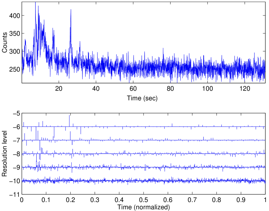
Figure 1: Data from GRB990308 with $z=1.60$ collected by BATSE trigger 7457 in a total number of $2^{11}$ $64$ ms bins in the energy band 115-320 keV (top panel), and its Symmlet-10 (Mallat  1998) discrete wavelet transform (DWT) at the level $L=6$. The horizontal axis corresponds to the same time scale as in the original burst. Each level on the vertical axis shows the wavelet coefficients at a given resolution level (i.e., scale). The wavelet coefficients are represented by spikes whose size and direction (up or down) is determined by the magnitude and sign (+ or -) of the coefficient.

The CWT is mostly used for the analysis and detection of signals, whereas the DWT is more appropriate for data compression and signal reconstruction. Combining these two types of wavelet transforms provides an advanced technique for picking up the positions of particular breaks in the structures of observed GRB light curves in different energy bands, which we use here to look for non-trivial medium effects on the propagation of photons due to quantum gravity.

Orthogonal wavelets Eq. (19) dilated by factors $2^{j}$ are sensitive to signal variations with resolutions $2^{-j}$. This property can be used to make a sequence of approximations to a signal with improving resolutions (e.g.   Mallat  1998). For a function satisfying the condition Eq. (20), the partial sum of wavelet coefficients $\sum_{k=-\infty}^{+\infty}d_{j,k}\psi_{j,k}$ can be interpreted as the difference between two approximations to $f$ with resolutions $2^{-j+1}$ and $2^{-j}$. Adapting the signal resolution allows one to process only the details relevant to a particular task, namely to estimate intensity profiles of GRB light curves preserving the positions of sharp signal transients.

CWTs can detect with very high precision the positions where the intensity profile of a GRB light curve, as estimated by a DWT, changes its degree of regularity. Since $\psi$ has zero average, a wavelet coefficient $Wf(u,s)$ measures the variation of $f$ in a neighborhood of $u$ whose size is proportional to $s$. Sharp signal transitions create large-amplitude wavelet coefficients. As we see in the following section, the pointwise regularity of $f$ is related to the asymptotic decay of the wavelet transform $Wf(u,s)$ when $s$ goes to zero. Singularities are detected by following across different scales the local maxima of the wavelet transform. We use this ‘zooming’ capability to define the positions of mathematically similar transients (irregularities) in GRB light curves observed in different energy bands. These therefore provide the best information about the arrival times of photons associated with universal intrinsic emission features at the sources.

4 Extraction of the GRB Intensity Profiles by Wavelet Shrinkage

The observed GRB light curves typically feature a relatively homogeneous, nonzero background intensity, above which some inhomogeneous structure is apparent (Kolaczyk  1997). In the following, we demonstrate that when such a temporally inhomogeneous signal as the light curve of a GRB contains both structure and noise, the ability of the DWT to compress the information in this signal leads efficiently to a simple but effective noise removal procedure. This wavelet shrinkage technique (Donoho  1993; Donoho et al. 1995), based on the thresholding of the DWT, allows one to separate the structure of the signal from the noise, whilst retaining information about the position of irregularities of the signal, as provided by the support of the mother wavelets.

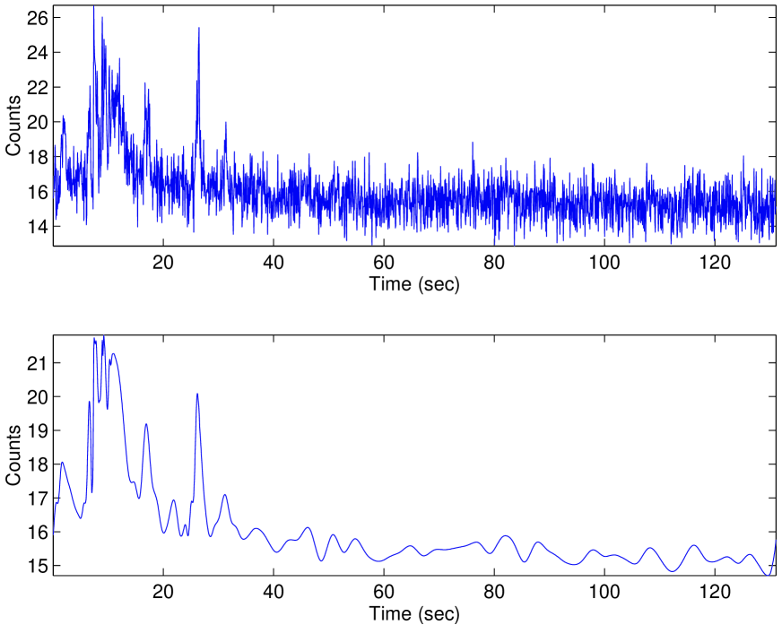
Figure 2: The GRB990308 light curve after preprocessing which sets the median absolute deviation of wavelet coefficients at the fine scale equal to unity, as described in more detail in Appendix 41. The intensity profile estimated by the wavelet shrinkage procedure at the level $L=6$ is presented in the bottom panel.

In practice, DWTs break a function down into a coarse approximation at a given scale, that can be extended to successive levels of residual detail on finer and finer scales. The full decomposition may be expressed in terms of the scale function $\phi_{j,n}$ and the discrete wavelet $\psi_{j,n}$ discussed already. The scale function looks much like a kernel function, and a finite linear combination of dyadic shifts of this function provides a generic coarse approximation. Further linear combinations of dyadic shifts of the wavelet function supply the residual detail. By considering sequences of DWTs with increasing numbers of dyadic dilatations, the detail at each of the corresponding successive scales is recovered.

We represent the light curve of a given GRB by a binned discrete signal $\{X_{0},X_{1},\dots,X_{n-1}\}$ of dyadic length $n=2^{J}$, where $J>0$. The DWT of such a signal results in a vector of length $n$ of wavelet coefficients. The signal is said to have been sampled at level $J$. At some coarser resolution level (scale) $L<J$, the wavelet coefficient vector contains $2^{L}$ scale coefficients $c_{L,0},\dots,c_{L,2^{L-1}}$ and $2^{j}$ detail coefficients $d_{j,0},\dots,d_{j,2^{j-1}}$ at each of the levels $j=L,\dots,J-1$. Fig. 1 displays a typical example with $J=11$ and $L=6$.

Observations of a given GRB light curve can be represented by the sum

$$X[n]=f[n]+W[n],$$ (21)

where the intensity profile $f[n]$ is contaminated by the addition of noise, which is modelled as a realization $W[n]$ of a random process whose probability distribution is known. The intensity profile $f$ is estimated by transforming the noisy data $X[n]$ with the ‘decision operator’ $D$:

$$\tilde{F}=DX.$$ (22)

The ‘risk’ of the estimator $\tilde{F}$ of $f$ is the average loss, calculated with respect to the probability distribution of the noise. The numerical value of the risk is often specified by the signal-to-noise ratio (SNR), which is measured in decibels.

To reduce the noise level of $W$, while preserving the degree of regularity of the intensity profile $f$, we use a soft thresholding procedure. This procedure sets to zero all coefficients smaller in magnitude than some threshold $T$, and shrinks coefficients larger than $T$ towards zero by amounts $T$, as described in more detail in Appendix 41. This performs an adaptive smoothing that depends on the regularity of the signal $f$. In a wavelet basis  where large-amplitude coefficients correspond to transient signal variations, this means that the estimator discussed in Appendix 41 keeps only transients coming from the original signal, without adding others due to the noise. After the preprocessing, which sets the median value of wavelet coefficients of the signal at the finest scale to unity, the threshold is estimated to be $T=\sqrt{2\log n}$. The example of an intensity profile estimated by this wavelet shrinkage procedure, as described in Appendix 41, is shown in Fig. 2.

In general, the wavelet shrinkage procedure Eq. (40) described above guarantees with high probability that $|d_{j,m}^{\tilde{F}}|\leq|d_{j,m}^{f}|$ (e.g.  Mallat  1998), implying that the estimator $\tilde{F}$ is at least as regular as the ‘original’ intensity profile $f$, because its wavelet coefficients have smaller amplitudes. Thus we use this property of the DWT of separating very effectively the structures in the GRB intensity profiles from noise, in the form of two subsets of wavelet coefficients, large and small ones. The thresholding procedure deletes wavelet coefficients below the threshold value, and diminishes the others by the threshold value. This tends to preserve both broad and narrow features, while significantly reducing noise fluctuations, after the reconstruction of the intensity profile by the inverse DWT.

5 Detection of Variation Points in GRB Light Curves

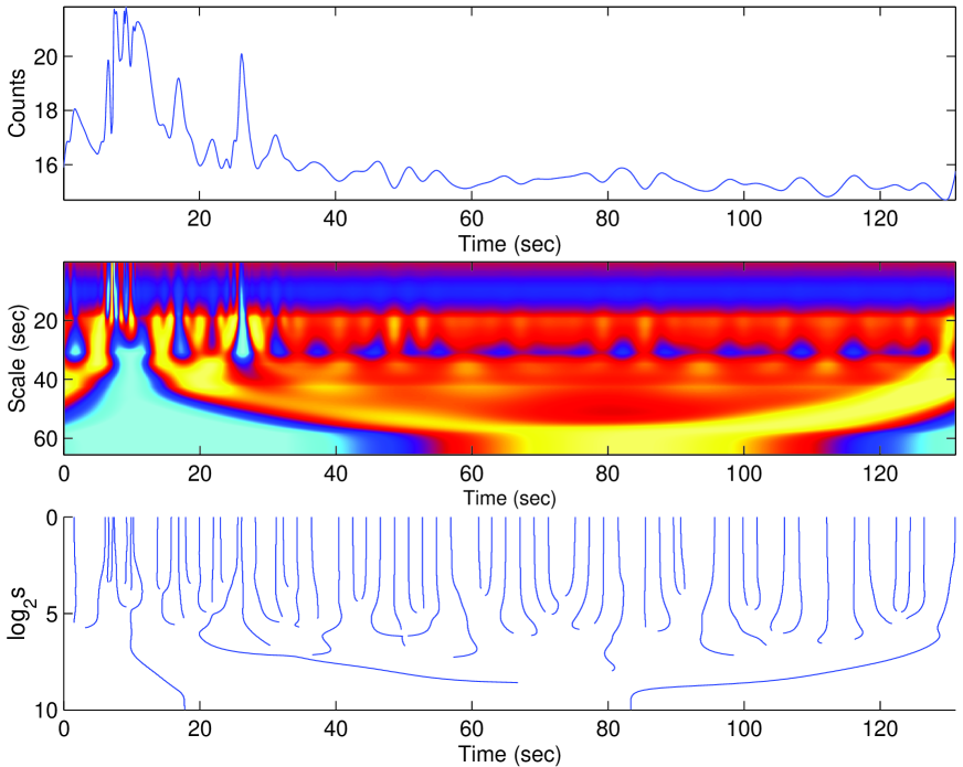
Figure 3: The CWT image (middle panel) of the GRB990308 intensity profile (top panel). The horizontal and vertical axes give, respectively, the position $u$ and $\log_{2}s$ (where $s$ is the time scale in seconds), The shadings (colours from yellow to blue) correspond to negative, zero and positive wavelet transforms respectively. Singularities create large amplitude coefficients in their cone of influence. The modulus maxima (bottom panel) of $Wf(u,s)$ obtained from the matrix of CWT (middle panel) pointing towards the time positions of singularities at the fine scale.

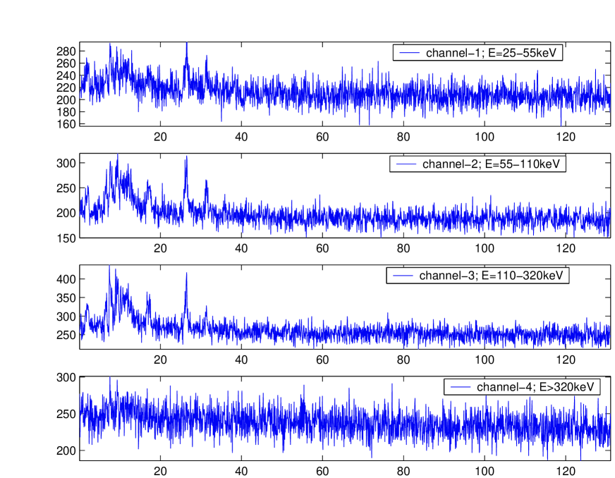
Figure 4: The light curve for GRB990308 obtained by BATSE with trigger 7457, binned with 64 ms resolution in four spectral bands.

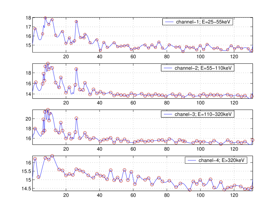
Figure 5: The estimated intensity profiles of GRB990308 - see Fig. 4 - obtained in four spectral bands by using a Symmlet-$10$ (Mallat  1998) basis at level $L=6$. The signal-to-noise ratios are at the levels $SNR1=23.07$, $SNR2=22.71$, $SNR3=23.58$ and $SNR4=23.87$ for each band, respectively. All variation points founded by CWT zoom are marked by circles. The behaviours of the Lipschitz exponents $\alpha$ are estimated. Seven pairs of genuine variation points in the first and third spectral bands have been detected.

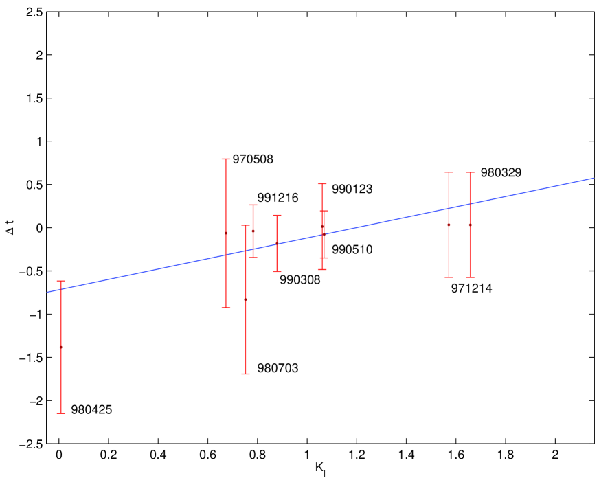
Figure 6: Spectral time lags between the arrival times of pairs of genuine variation points detected in the third and first BATSE spectral bands. The analysis has been done for 9 GRB light curves collected with time resolution 64 ms. The solid line shows the best linear fit versus $K_{\rm l}$.

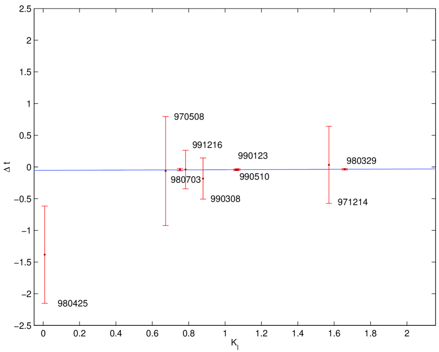
Figure 7: The combination of $64$ ms BATSE time-lag measurements shown in Fig. 6 with the measurement obtained from the BATSE-OSSE comparison and the TTE portion of the GRB980329 light curve, with resolution 2.7 ms.

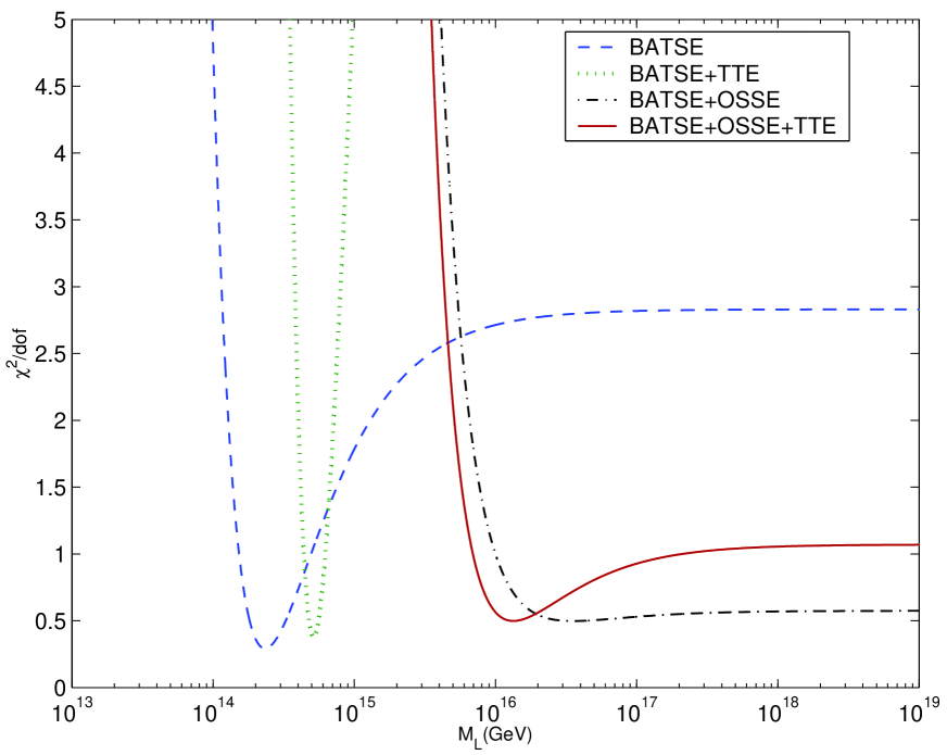
Figure 8: The $\chi^{2}$ function defined in Eq. (35) as a function of the quantum gravity scale, for the scenario with a linear energy dependence of the vacuum refractive index, as obtained using different combinations of data sets. The solid line, which is used to establish the lower limit Eq. (36), corresponds to the combination of $64$ ms BATSE data with both TTE and OSSE-BATSE data.

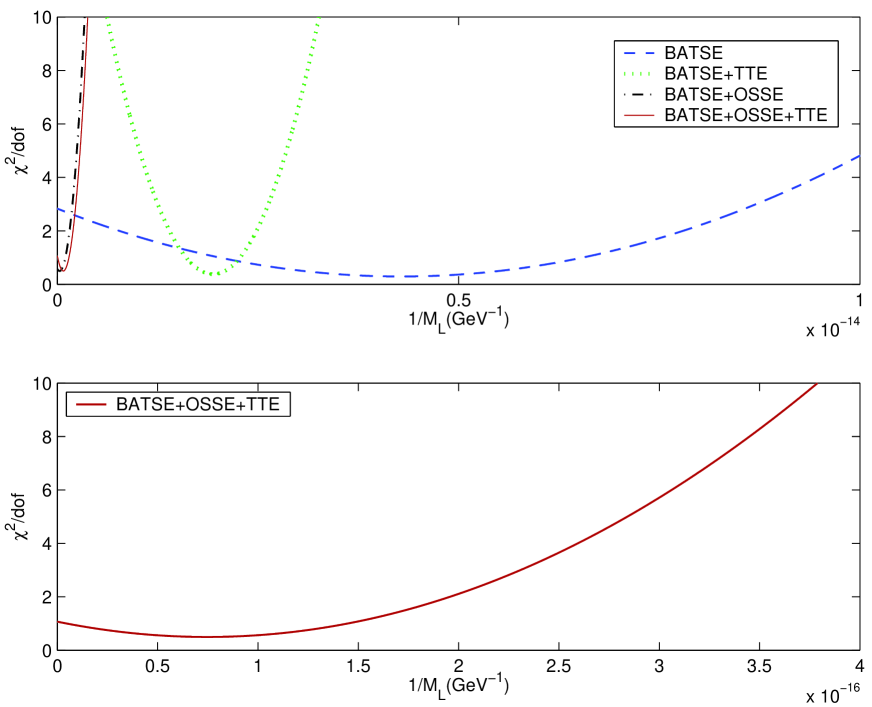
Figure 9: The same $\chi^{2}$ function as in Fig. 8, which is defined in Eq. (35), now plotted as a function of the inverse quantum-gravity scale. The solid line corresponds the final lower limit Eq. (36).

A wavelet transform can focus on localized signal structure via a ‘zooming’ procedure that reduces progressively the scale parameter. To identify the variability points of two different light curves and characterize their structures, it is necessary to quantify precisely the local regularity of the function which represents the intensity profile of the original signals. The appropriate tools are the Lipschitz exponents . These are defined in Appendix 43, and can provide uniform regularity measurements of a function $f$ not only over time intervals, but also at any point $\nu$.

We use the Lipschitz exponent $\alpha$ to characterize variation points of the reconstructed intensity profiles of GRBs accumulated in different energy bands. The comparison of the positions of variation points with the same values of $\alpha$ gives the information about the arrival times of photon probes with different energies, enabling one to probe for quantum-gravity time-delay phenomena.

The decay of the CWT amplitude as a function of scale is related to the uniform and pointwise Lipschitz regularity of the signal. Thus, measuring this asymptotic decay is equivalent to ‘zooming’ into signal structures with a scale that goes to zero. Namely, when the scale $s$ decreases, the CWTs $Wf(u,s)$ Eq. (15) measures fine-scale variations in the neighborhood of $u$. One can prove (e.g. Mallat  1998) that $|Wf(u,s)|$ decays like $s^{\alpha+1/2}$ over intervals where $f$ is uniformly Lipschitz $\alpha$. Furthermore, the decay of $|Wf(u,s)|$ can be controlled from its local maxima values.

A ‘modulus maximum’ (e.g. Mallat  1998) is any point $(u_{0},s_{0})$ such that $|Wf(u,s_{0})|$ is locally maximal at $u=u_{0}$. This local maximum should be a strict local maximum in either the right or the left neighborhood of $u_{0}$. Any connected curve $s(u)$ in the scale-time plane $(u,s)$ along which all points are modulus maxima, as illustrated in Fig. 3, is called a ‘maxima line’. Singularities of a function $f$ are detected by finding the abscissa where the wavelet modulus maxima converge on fine scales (e.g. Mallat  1998). Only at such points can $f$ be singular, i.e., with exponent $\alpha\leq 1$. This result guarantees that all singularities are detected by following the wavelet transform modulus maxima at fine scales. Fig. 3 shows an example where all the significant singularities are located by following the maxima lines. The positions of these singularities are located by the modulus maxima lines at the fine scale of decomposition.

To be sensitive to both sharp and smooth singularities, one has to use wavelets with two vanishing moments, so as to generate the CWT Eq. (15) of the reconstructed intensity profiles. The most suitable one is the second derivative of a Gaussian (Mexican hat) mother wavelet:

$$\Psi(t)=\frac{2}{\pi^{1/4}\sqrt{3\sigma}}\left(\frac{t^{2}}{\sigma^{2}}-1\right)\exp\left(-\frac{t^{2}}{2\sigma^{2}}\right),$$ (23)

because of the property that the modulus maxima of $Wf(u,s)$ with the wavelet Eq. (23) belong to connected curves that are not broken as the scale $s$ decreases (e.g. Mallat  1998), which guarantees that all maxima lines propagate to the finest scales. The dilatation step $s$ is generally set to $s=2^{1/\Delta}$, where $\Delta$ is the number of intermediate scales (voices) for each octave. Thus, if the voice lattice is sufficientely fine, one can build maxima lines with very high precision. Connecting maxima into lines as in Fig. 3 is a procedure for removing spurious modulus maxima created by numerical errors in regions where the CWT is close to zero.

Sometimes the CWT may have a sequence of local maxima that converge to a point $\nu$ on the abscissa, even if $f$ is perfectly regular at $\nu$. Thus, to detect singularities it is not sufficient merely to follow the wavelet modulus maxima across the scales. One must also calculate the Lipschitz regularity from the decay of the modulus maxima amplitude. If, for some scale $s<s_{0}$, all the modulus maxima that converge to $\nu$ are included in a cone:

$$|u-\nu|\leq Cs,$$ (24)

then $f$ has an isolated singularity at $\nu$. Conversely, the absence of maxima below the cone of influence Eq. (24) implies that $f$ is uniform in the neighborhood of any point $t\neq\nu$ beyond the scale $s_{0}$.

The Lipschitz regularity at $\nu$ is given by the slope $\log_{2}|Wf(u,s)|$ as a function of $\log_{2}s$ along the maxima lines converging to $\nu$, namely

$$\log_{2}|Wf(u,s)|\approx\left(\alpha+\frac{1}{2}\right)\log_{2}s+const.$$ (25)

Actually, the Lipschitz property Eq. (42) approximates a function with a polynomial $p_{\nu}$ in the neighborhood of the point $\nu$. The CWT estimates the Lipschitz exponents of the function by ignoring the polynomial $p_{\nu}$ itself. Moreover, if the scale $s_{0}$ is smaller then the distance between two consecutive singularities, to avoid having other singularities influence the value of $Wf(u,s)$, and the estimated Lipschitz exponent $\alpha+1/2\leq 1.5$, the function $f$ exhibits a break at $\nu$, which can be detected by following the modulus maxima chain.

In this paper, to define significant points in the time series of the signal, we do not apply fit functions that select only prominent peaks, as was done in (Ellis et al. 2000b; Norris et al. 1995). We consider a more general class of relatively sharp signal transitions, marked by Lipschitz irregularities picked out by the CWT ‘zoom’ technique, which we call genuine variation points.

GRB (BATSE Trigger)	$z$	Time lag, error (s)
970508 (6225)	0.835	BATSE (64 ms)
		$\Delta t_{1}^{\rm BATSE}=-0.064$ $\pm 0.860$
971214 (6533)	3.418	BATSE (64 ms)
		$\Delta t_{1}^{\rm BATSE}=0.13$ $\pm 0.860$; $\Delta t_{2}^{\rm BATSE}=-0.064$ $\pm 0.860$
		cobmbined BATSE (64 ms)
		$\Delta t_{\rm comb}^{{\rm BATSE}}=0.033$ $\pm 0.608$
980329 (6665)	$3.9$	BATSE (64ms)
		$\Delta t_{1}^{{\rm BATSE}}=0.064$ $\pm 0.860$; $\Delta t_{2}^{{\rm BATSE}}=0$ $\pm 0.860$
		combined BATSE (64 ms)
		$\Delta t_{\rm comb}^{{\rm BATSE}}=0.032$ $\pm 0.608$
		BATSE-TTE (2.7 ms)
		$\Delta t_{1}^{\rm TTE}=-0.34$ $\pm 0.019$
		OSSE (64 ms) rescaled
		$\Delta t_{1}^{{\rm OSSE}}=-0.048$ $\pm 0.019$; $\Delta t_{2}^{{\rm OSSE}}=0$ $\pm 0.038$
		combined BATSE+OSSE+TTE
		$\Delta t_{\rm comb}^{{\rm BATSE+rmOSSE+TTE}}=-0.036$ $\pm 0.013$
980425 (6707)	0.0085	BATSE (64 ms)
		$\Delta t_{1}^{{\rm BATSE}}=-1.792$ $\pm 1.705$; $\Delta t_{2}^{{\rm BATSE}}=-1.28$ $\pm 0.860$
		combined BATSE (64 ms)
		$\Delta t_{\rm comb}^{{\rm BATSE}}=-1.384$ $\pm 0.768$
980703 (6891)	0.966	BATSE (64 ms)
		$\Delta t_{1}^{{\rm BATSE}}=-0.832$ $\pm 0.860$
		OSSE (64 ms) rescaled
		$\Delta t_{1}^{{\rm OSSE}}=-0.040$ $\pm 0.019$
		combined BATSE+OSSE
		$\Delta t_{\rm comb}^{\rm BATSE+OSSE}=-0.041$ $\pm 0.019$
990123 (7343)	1.600	BATSE (64 ms)
		$\Delta t_{1}^{{\rm BATSE}}=0.230$ $\pm 0.860$; $\Delta t_{2}^{{\rm BATSE}}=-0.064$ $\pm 0.860$; $\Delta t_{3}^{{\rm BATSE}}=-0.128$ $\pm 0.860$
		combined BATSE (64 ms)
		$\Delta t_{\rm comb}^{{\rm BATSE}}=0.013$ $\pm 0.496$
		OSSE (64 ms) rescaled
		$\Delta t_{1}^{{\rm OSSE}}=-0.049$ $\pm 0.019$; $\Delta t_{2}^{{\rm OSSE}}=-0.046$ $\pm 0.019$; $\Delta t_{3}^{{\rm OSSE}}=-0.045$ $\pm 0.019$
		combined BATSE+OSSE
		$\Delta t_{\rm comb}^{\rm BATSE+OSSE}=-0.047$ $\pm 0.011$
990308 (7457)	1.2	BATSE (64 ms)
		$\Delta t_{1}^{{\rm BATSE}}=0$ $\pm 0.860$; $\Delta t_{2}^{{\rm BATSE}}=-0.064$ $\pm 0.860$; $\Delta t_{3}^{{\rm BATSE}}=-0.256$ $\pm 0.860$
		$\Delta t_{4}^{{\rm BATSE}}=-1.024$ $\pm 0.860$; $\Delta t_{5}^{{\rm BATSE}}=0$ $\pm 0.860$; $\Delta t_{6}^{{\rm BATSE}}=0.064$ $\pm 0.860$
		$\Delta t_{7}^{{\rm BATSE}}=0$ $\pm 0.860$
		combined BATSE (64 ms)
		$\Delta t_{\rm comb}^{{\rm BATSE}}=-0.183$ $\pm 0.325$
990510 (7560)	1.619	BATSE (64 ms)
		$\Delta t_{1}^{{\rm BATSE}}=0.384$ $\pm 0.860$; $\Delta t_{2}^{{\rm BATSE}}=0.448$ $\pm 0.860$; $\Delta t_{3}^{{\rm BATSE}}=0$ $\pm 0.860$
		$\Delta t_{4}^{{\rm BATSE}}=-0.256$ $\pm 0.860$; $\Delta t_{5}^{{\rm BATSE}}=0$ $\pm 0.860$; $\Delta t_{6}^{{\rm BATSE}}=-0.528$ $\pm 0.860$
		$\Delta t_{7}^{{\rm BATSE}}=-0.128$ $\pm 0.860$; $\Delta t_{8}^{{\rm BATSE}}=-0.256$ $\pm 0.860$; $\Delta t_{9}^{{\rm BATSE}}=0$ $\pm 0.860$
		$\Delta t_{10}^{{\rm BATSE}}=-0.448$ $\pm 0.860$
		combined BATSE (64 ms)
		$\Delta t_{\rm comb}^{{\rm BATSE}}=-0.078$ $\pm 0.272$
		OSSE (64 ms) rescaled
		$\Delta t_{1}^{{\rm OSSE}}=-0.045$ $\pm 0.019$; $\Delta t_{2}^{{\rm OSSE}}=-0.032$ $\pm 0.019$; $\Delta t_{3}^{{\rm OSSE}}=-0.041$ $\pm 0.019$
		combined BATSE (64 ms)
		$\Delta t_{\rm comb}^{{\rm BATSE+OSSE}}=-0.039$ $\pm 0.011$
991216 (7906)	1.02	BATSE (64 ms)
		$\Delta t_{1}^{{\rm BATSE}}=-0.064$ $\pm 0.860$; $\Delta t_{2}^{{\rm BATSE}}=-0.064$ $\pm 0.860$; $\Delta t_{3}^{{\rm BATSE}}=-0.064$ $\pm 0.860$
		$\Delta t_{4}^{{\rm BATSE}}=-0.064$ $\pm 0.860$; $\Delta t_{5}^{{\rm BATSE}}=0.064$ $\pm 0.860$; $\Delta t_{6}^{{\rm BATSE}}=0$ $\pm 0.860$
		$\Delta t_{7}^{{\rm BATSE}}=0$ $\pm 0.860$; $\Delta t_{8}^{{\rm BATSE}}=0$ $\pm 0.860$
		combined BATSE (64 ms)
		$\Delta t_{\rm comb}^{{\rm BATSE}}=-0.040$ $\pm 0.304$

Table 1: Data on the light curves for GRBs with known redshifts used in this analysis. The third column gives the time lags between the arrivals of every identical genuine variation points in the third (high-energy) spectral band and the first (low-energy) one. For every light curve, we give the weighted means of the time lags in $64$ ms BATSE domain, combining the genuine variation points for that GRB. Both statistical and systematic errors are included. The average spread of individual time lags is below the mesurement uncertainty. Also indicated are the results obtained by combining OSSE $64$ ms light curves in the $3$–$6$ MeV energy range with BATSE light curves in the $115$–$320$ keV energy band. In the case of GRB980329, the results of BATSE $64$ ms and TTE $2.7$ ms resolution measurements are combined with the OSSE-BATSE $64$ ms comparisons.

6 Analysis of Time Lags in Emissions from GRBs with Known Redshifts

Once the BeppoSAX satellite began to localize long bursts in the sky to within a few arcminutes, and distribute their locations to observers within hours, it turned to be possible to discover X-ray, optical, and radio afterglows (Costa et al. 1997; van Paradijs et al. 1997; Frail et al. 1997), and host galaxies. Subsequent observations led to the spectroscopic determination of GRB redshifts, using absorption lines in the spectra of the afterglows and emission lines in the spectra of the host galaxies. By now, redshifts have been measured for about 20 bursts (see for example (Norris et al. 2000; http://www.aip.de/${\tilde{\leavevmode\nobreak\ }}$jcg/grbrsh.html; Amati et al. 2002) and references therein).

Our first aim is to measure the timings of genuine variation points, characterized by Lipschitz exponents as discussed above, for different spectral bands in the light curves of distant GRBs. Correlating the time lags between different energies with the GRB redshifts, we then try to extract time delays related to the refractive index that may be induced by quantum gravity.

We use genuine variation points with the same Lipschitz exponents $\alpha$, measured in different energy bands, and assume that any initial relative time lags attributable to the properties of source are independent of redshift. Thus, the key to disentangling quantum-gravity effects is reduced to the problem of detecting genuine variation points with the highest possible precision. The biggest uncertainties in our analysis come from our procedure for estimating the DWT intensity profiles, whilst the errors generated by the CWT zoom are negligible. The error in the wavelet-shrinkage procedure is defined by the time-bin resolution in the analysis of the light curve and the support of the DWT mother wavelet.

As shown in Table 1, we use GRB light curves from BATSE, which have been recorded with 64 ms temporal resolution in four spectral channels. Unfortunately, the BATSE catalog of light curves includes only about a half of the GRBs with known redshifts. The light curves of the other GRBs with known redshifts have been collected by other satellites (BeppoSAX, HETE), and the data are not available publicly. The BATSE lower-level discriminator edges define the channel boundaries at approximately 25, 55, 115 and 320 keV. We look for the spectral time lags of the light curves recorded in the $115-320$ keV energy band relative to those in the lowest $25-55$ keV energy band, providing a maximal lever arm between photon energies. We do not use the fourth BATSE channel with energies between $320$ keV and $1.9$ MeV, as these have ill-defined energies and poorer statistics - see Fig. 4. Instead, we compare the rather more energetic light curves accumulated by OSSE  with the $115-320$ keV BATSE light curves, which increases the lever arm for probing photon propagation into the MeV range.

Since we apply the CWT zoom technique to detect the genuine variation points of the reconstructed intensity profiles, we impose some conditions on the choice of shrinking wavelet . In general, when choosing the appropriate wavelet basis, one has to strike a balance between the degree of regularity of the wavelet, the number of its vanishing moments $p$ and the size of its support. It is clear that the size of the support defines uncertainties in the positions of genuine variation points after the reconstruction of intensity profile. This consideration motivates using the DWT basis with the most compact support for the wavelet shrinkage procedure. On the other hand, to preserve maximally the regularity of the original signal, one should use wavelets with a high degree of regularity. In addition, one should avoid disturbing significantly the alignment of peaks of the original light curves, which motivates using symmetrical discrete wavelets.

The discrete wavelet that best reconciles the above requirements is that called Symmlet-$p$ (e.g. Mallat  1998). It is the most symmetric, regular discrete wavelet with minimum support. The number $p$ of vanishing moments defines the size of the support, and consequently the errors of the position estimations $\frac{1}{2}(2p-1)\times{\rm bin-size}$. Moreover the same number $p$ of vanishing moments defines the regularity of Symmlet-$p$. For a large number of vanishing moments, the Lipschitz regularity of Symmlet-$p$ is $0.275p$ (Daubechies  1991). Thus, to have more then $2$ continuous derivatives, $p$ should exceed $8$.

For the selected GRBs in Table 1, we have performed the wavelet shrinkage procedure using a Symmlet-$10$ basis . At sufficiently high signal-to-noise ratio levels, this procedure tends to preserve the regularity of the light curves. In some cases, namely for GRB980329 and GRB970508, we applied the translation-invariant (Mallat  1998) version of the shrinkage procedure with reduced threshold. This procedure implies averaging estimates produced from the original signal itself and from all shifted versions of the signal, and allows one to avoid artefacts while preserving the real transient structure. Subsequently, we apply the CWT zoom technique for reconstructing intensity profiles to identify the arrival times of genuine variation points and estimate their Lipschitz exponents in every spectral band. We consider that a genuine variation point has been detected if it has Lipschitz exponent $\alpha\leq 1$. Genuine variation points found in the vicinity of each other, but belonging to two different spectral bands, are considered to have been generated at the source if the values of their Lipschitz exponents are equal to each other. The other variation points with $\alpha$ substantially exceeding $1$ exhibit only smooth transitions of the signal, and do not mark sharp transient time structures. We recall that only sharp transient structures are important in the search for spectral time lags. For seven GRBs out of nine, we detected more than one pair of identical genuine variation point per light curve, as seen in Table 1. The systematic errors (Kolaczyk  1997) were estimated by using different resolution levels ($L=6,\ 5,\ 4$) in the wavelet shrinkage procedure.

In order to probe the energy dependence of the velocity of light that might be induced by quantum gravity, we have compiled the whole available data in Table 1 as functions of the variables $K_{\rm l}$ and $K_{\rm q}$, defined by the integrals in Eq. (13) and Eq. (14), respectively. In the case of linear quantum-gravity corrections, the variable takes the form

$$K_{\rm l}=\int\limits_{0}^{z}\frac{dz}{h(z)},$$ (26)

whilst for the quadratic case we use

$$K_{\rm q}=\int\limits_{0}^{z}\frac{(1+z)dz}{h(z)}.$$ (27)

Since both Eq. (13) and Eq. (14) exhibit linear dependences on the variables Eq. (26) and Eq. (27) respectively, we perform a regression analysis for a linear dependence of the time lags between pairs of genuine variation points, in the form

$$\Delta t=aK+b.$$ (28)

The result of our regression fit to the full 64 ms statistics for linear quantum-gravity corrections Eq. (4) is shown in Fig. 6. The best fit corresponding to Fig. 6 is given by

$$\Delta t=0.60(\pm 0.46)K_{\rm l}-0.72(\pm 0.53).$$ (29)

Following the same procedure for the quadratic corrections, one gets

$$\Delta t=0.17(\pm 0.17)K_{\rm q}-0.42(\pm 0.32).$$ (30)

More precise results can be obtained by combining BATSE and OSSE data. Four light curves accumulated by OSSE exibit structures that can be compared with similar features observed by BATSE, as seen in Table 1. Since the OSSE data are at higher energies: $0.15-10$ MeV, one has to rescale the results of OSSE-BATSE comparison in order to combine them directly with results obtained using the third BATSE channel, by a factor:

$$\frac{110\leavevmode\nobreak\ {\rm keV}-55\leavevmode\nobreak\ {\rm keV}}{3\leavevmode\nobreak\ {\rm MeV}-110\leavevmode\nobreak\ {\rm keV}},$$ (31)

where $3\leavevmode\nobreak\ {\rm MeV}$ is the energy at which the contribution of flux accumulated by OSSE becomes significant. The spectral information for GRB980123 indicate that half of the total flux has been accumulated in the energy range $3-6$ MeV.

One may also increase the sensitivity of the determination of time lags by using BATSE time-tagged event (TTE) data, which record the arrival time of each photon with a precision of $2\leavevmode\nobreak\ \mu$s, in the same four energy channels. The onboard memory was able to record up to 32,768 photons around the time of the BATSE trigger. Typically, this quota of photons was filled in 1 or 2 s. For short GRBs, the mean structure of the whole light curve might be in the TTE data, along with substantial periods of background emission after the burst, whilst for the long-duration GRBs that we analyze, as in Table 1, the TTE data cover only the leading portion of light curve. We have rebinned with resolution $\simeq 1$ ms the leading portions of all the GRBs from Table 1 using TTE data. Only one light curve, that of GRB980329, yields a signal with clearly identified isolated singularities in the first and third spectral bands. The statistics available to detect genuine variation points in this light curve yield a resolution of 2.7 ms. Combining this TTE measurement with the 64 ms BATSE measurements and the results of our BATSE-OSSE comparisons, we get the following results:

$$\Delta t=0.010(\pm 0.022)K_{\rm l}-0.053(\pm 0.026)$$ (32)

$$\Delta t=0.003(\pm 0.006)K_{\rm q}-0.048(\pm 0.016)$$ (33)

for linear Fig. 7 and quadratic corrections respectively. The single BATSE point with much higher precision than the others does not improve substantially the significance of the fits. However, including the OSSE-BATSE and TTE measurements into the overall fit does improve the sensitivity (see the next section) and makes the result less dependent on the properties of individual sources.

The leading parts of other light curves from Table 1. which do not exhibit coherently variable structures, can be characterized as fractal signals without isolated singularities. One can also analyze such singularities with CWT (e.g. Dremin et al. 2001; Mallat  1998), but such a study lies beyond the scope of this paper.

7 Compilation of Limits on Quantum Gravity

We now analyze the likelihood function to derive the results of our search for a vacuum refractive index induced by quantum gravity. We establish a 95 % confidence-level lower limit on the scale $M$ of quantum gravity by solving the equation

$$\frac{\int\limits_{M}^{\infty}L(\xi)d\xi}{\int\limits_{0}^{\infty}L(\xi)d\xi}=0.95$$ (34)

where $\infty$ symbolizes a reference point fixing the normalization. In our case, we choose as reference point ${\cal M}=10^{19}$ GeV, the Planck mass, which corresponds to the highest possible scale above which quantum-gravity effects vanish and corrections to the vacuum refractive index become infinitesimally small. In practice variations of reference point, even by an order of magnitude, does not influence the final result.

We use the fact that only the coefficient $a$ in Eq. (28) is related to the quantum-gravity scale, whereas $b$ includes a possible unknown spectral time lag inherited from the sources, which we assume to be universal for our data set. With this assumption, one can shift our data points by an amount $-b$, taking $b$ from the best fits Eq. (29) and Eq. (30), and use $L\propto\exp(-\chi^{2}(M)/2)$ (with normalisation appropriately fixed to unity) as the likelihood function in Eq. (34), where

$$\chi^{2}(M)=\sum\limits_{\cal D}\left[\frac{\Delta t_{i}-b_{\rm shift}-a(M)K_{i}}{\sigma_{i}}\right]^{2}$$ (35)

is calculated for all the possible values of $a(M)$, defined by the coefficients of $K_{\rm l}$ ($K_{\rm q}$) in Eq. (13) and Eq. (14), respectively. The sum in Eq. (35) is taken over the all the data points $\Delta t_{i}$, which are symbolized by ${\cal D}$, with $\sigma_{i}$ characterizing the uncertainties in the measured time lags. The calculated $\chi^{2}(M_{\rm L})$ for the different combinations of the data sets we use in the case of linear corrections to the refractive index Eq. (14) is shown in Fig. 8. The minima of $\chi^{2}$ correspond the ‘signal-like’ regions, where the data are better described by a scenario with a refractive index, induced by quantum gravity. The most robust estimation on the lower limit of quantum gravity with a linearly energy-dependent correction is obtained from the combination of all the data sets, and is indicated by a solid line in Fig. 8:

$$M_{\rm L}\geq 6.9\cdot 10^{15}\leavevmode\nobreak\ {\rm GeV}$$ (36)

Similar considerations lead to the following lower limit on quadratic quantum-gravity corrections Eq. (5) to the photon dispersion relation:

$$M_{\rm Q}\geq 2.9\cdot 10^{6}\leavevmode\nobreak\ {\rm GeV}.$$ (37)

To the accuracy stated, we find identical numerical results, whether we use a logarithmic measure for $M$ cut off at ${\cal M}=10^{18,19,20}$ GeV, as shown in Fig. 8, or a $1/M$ measure integrated to infinity,

$$\frac{\int\limits_{0}^{1/M}L^{\prime}(\xi)d\xi}{\int\limits_{0}^{\infty}L^{\prime}(\xi)d\xi}=0.95,$$ (38)

where $L^{\prime}(1/M)$ is the likelihood function with respective to $1/M$, as shown in Fig. 9.

The key result (36) is significantly stronger than that in (Ellis et al. 2000b), thanks to the improved analysis technique using wavelets and the use of a more complete dataset.

8 Discussion

We have investigated in this paper possible non-trivial properties of the vacuum induced by quantum gravity, by probing modifications of the dispersion relation for photons. These features can appear in several approaches to quantum gravity, including Liouville string theory, models with large extra dimesions (Campbell-Smith et al. 1999) and loop gravity. Similar modifications of dispersion relations can take place for the other matter particles, leading to other non-trivial effects such as changes in the thresholds for some reaction attenuating ultra-high energy cosmic rays (UHECR), or vacuum Čerenkov-like radiation (see (Sarkar  2002) and references therein), which could have a large influence on the interpretation of the puzzling astrophysical data on UHECR.

We have attempted to extract the most complete information about the possible vacuum refractive index induced by quantum gravity, by using wavelets to look for any correlation with redshift of the time lags between the arrival times of sharp transients in GRB light curves observed in high- and low-energy spectral bands. This analysis combined continuous wavelet transforms to remove noise and discrete wavelet transforms to identify sharp transients in different spectral bands. Eight GRBs with known cosmological redshifts and light curves available publicly have been used in our analysis.

It is instructive to compare the time lags we find with those found using cross-correlation analysis (Band  1997; Norris et al. 2000; Norris  2002). Our measurements of the spectral time lags in BATSE $64$ ms light curves for five GRBs, which are common for the sample we used and that under consideration in Norris et al. 2000, are consistent in absolute value with the trend found in Norris et al. (2000) for bursts with higher luminosities (which are closer, on the average) to have shorter time lags. Discrepancies are found in two cases out of five common GRBs. Namely, we found soft-to-hard evolution for GRB971214 and GRB990123 (positive time lag), which is opposite to the hard-to-soft evolution (negative time lag) found in Norris et al. 2000. These two GRBs havea complicated structure of emission: GRB971214 has a wide “clump” of emission which consists of spikes that are barely overlapped, while GRB990123 consists; in two intensive wide pulses with a quite complicated cluster afterwards. Thus these two GRBs can be attributed to a lack of morphological classification power of the cross-correlation technique due to the problem of interpretation of the CCF pike width (Band  1997). As an explicit example, we analysed GRB941119, which has been assigned, in Band  1987, as the GRB without clear spectral evolution with the respective to cross-correlation analyses. The light curve of GRB941119 consists in cluster with several closely spaced spikes protruding from a smooth envelope. We found five pairs of identical genuine variation points in first and third spectral bands, demonstrating all together the soft-to-hard spectral evolution with weghted average time lag $\Delta t=0.051\pm 0.384$ s. One can see from Table 1 that in several cases different pairs of identical genuine variation points detected in one and the same GRB’s light curve demonstrate different kinds of spectral evolution, namely either hard-to-soft or soft-to-hard. This fact could be connected with a possible intrinsic spectral evolution during the burst progress. The example of GRB941119 is one of such cases, demonstrating unclear spectral evolution with the respect to the cross-correlation analysis. The wavelet technique we apply classifies more explicitly a variable spectral evolution and consequently gives more accurate results for the weighted average spectral evolution, as in case of GRB941119. The time lags measured between the BATSE 25-55 keV and OSSE 3-6 MeV light curves exceed substantially the time lags between the first and third BATSE energy bands. Without the correction by the ratio Eq. (31), the BATSE-OSSE time lags we find are $\simeq-2$ s, in good agreement with Piro et al.1998, where the time lag between bands of GRB970228 with a similar energy difference was estimated using BeppoSAX data. The wavelet technique is very effective also to deal with transient signals such as TTE data with low signal-to-noise ratios, where cross-correlation analyses can fail.

We believe that there is no regular cosmological evolution of the sources we use. This fact is already widely accepted in the literature on other high-redshift sources, namely supernovae. So there is no effect that can cause any correlation of weighted average time lags with redshifts of the sources. Thus any correlation of spectral time lags we may find can be attributed to the effects of propagation.

Finally it should be stressed that the method we applied is very powerful in the sense of analysing signals with strong non-linear dynamics behind, as GRBs could be. Of course it does not pretend to explain the underlying dynamics and physical origin of GRBs, but it gives a hint of the stage at which the most variable processes take place and characterize quantitatively the degree of instability accompanying those processes. In our case the radiation from genuine variation points is considered as the messenger of a fast non-linear dynamics at the source. The Lipschitz exponents, which characterize quantitatively the ‘degree’ of instability of the dynamics, give the information of whether photons of different energies have been produced at one and the same event at the source. So this gives an ideal ’time offset’ between energy bands to measure any differences in the speed of light.

It is widely accepted (see Band et al. 1997; Norris et al. 2000, and references therein) that the spectral evolution in GRBs leads to peaks migrating later in time. These time lags are not directly connected with the distance to the source, but are correlated with intrinsic properties of GRBs, such as luminosity (Norris et al. 2000) or variability (Shaefer et al. 2001). The quantum-gravity energy-dependent time delay plays the role of a foreground effect of opposite sign to the usual spectral evolution of GRBs, which increases with distance. Hence model-independent information about quantum gravity can be extracted only from a statistical analysis of sources with a known distance distribution.

We have not found a significant correlation of the measured time lags with the cosmological redshift that would indicate any deviation of the vacuum refractive index from unity. This fact allows us to establish 95 % C.L. lower limits on the quantum-gravity scale at the levels $6.9\cdot 10^{15}$ GeV and $2.8\cdot 10^{6}$ GeV for linear and quadratic distortions of the dispersion relation, respectively. However, despite the lack of any significant evidence for a quantum-gravity signal, there is a region of the linear scale parameter $M$ where the data are better described by a scenario with a refractive index induced by quantum gravity. This fact indicates that any increase in the statistics, especially with higher resolution, would be of the utmost interest for exploring the possibility of a quantum-gravity correlation of spectral time lags with redshift. For this reason, we urge the light curves for all GRBs with measured redshifts to be made generally available, as is already the case for BATSE data.

It has been observed that, if the dispersion laws for elementary particles differ from the standard ones, the expansion of the Universe may result in the gravitational creation of pairs of particles and antiparticles with very high energies (Starobinsky & Tkachev  2002). The expansion of the Universe (both at present and in the early Universe) gradually redshifts Fourier modes of a quantum field, and may transport them from the trans-Planckian region of very high momenta to the sub-Planckian region where the standard particle interpretation is valid. Then, if the WKB condition is violated somewhere in the trans-Planckian region, the field modes enter the sub-Planckian region in a non-vacuum state containing equal numbers of particles and antiparticles. The most restrictive upper limit follows from the number of UHECR created at the present epoch (Starobinsky & Tkachev  2002). This limit, together with our measurements of the vacuum refractive index, may rule out the possibility of detecting imprints of trans-Plankian physics on the CMB anisotropy, as proposed in (Brandenberger & Martin  2002).

It is a widespread belief that the combination of quantum theory with gravity is an explosive area, to the extent that it blows up the concrete fabric of space-time, splitting it into space-time foam. It is true that, as yet, there is no universally accepted mathematical model of this metamorphosis, while several attempts at it are characterized by a varying level of success. However, despite the firm and widely-held opinion that quantum gravity defies experimental tests, it is remarkable that several such tests have been proposed in recent years. Some of them have put rather severe constraints on some quantum-gravity models, whilst some models based on non-critical strings seem to remain unscathed so far (Ellis et al. 2002; Ellis et al. 2002a). In particular, as we have shown in this paper, using the most sophisticated technique available, that of wavelets, to pick up authentic time-lag effects in gamma-ray bursts, we have been able to put a rather firm lower bound on the dispersion of light in the vacuum: $M>6.9\times 10^{15}$ GeV. This approaches the range of scales where we might expect such an effect to appear. Data able to test further this possibility already exist, and more data will soon be available.

Une affaire à suivre ….

Appendix A Wavelet-Based Thresholding Estimator

A thresholding estimator of a $n=2^{J}$-component discrete signal $X[n]$ decomposed at the resolution level $L$ (see Section 4) in a wavelet basis can be written (Mallat  1998) as:

$$\tilde{F}=\sum\limits_{j=L}^{J-1}\sum\limits_{m=0}^{2^{j-1}}\rho_{T}(d_{j,m}^{X})\psi_{j,m}+\sum\limits_{m=0}^{2^{L-1}}\rho_{T}(c_{J,m}^{X})\phi_{J,m},$$ (39)

where the function $\rho_{T}$ provides a soft threshold:

$$\rho_{T}(x)=\left\{\begin{array}[]{lcl}x-T&{\rm if}&x\geq T\\ x+T&{\rm if}&x\leq-T\\ 0&{\rm if}&|x|\leq T\end{array}\right.$$ (40)

If the signal $X[n]$ is contaminated by additional noise $W[n]$, the threshold $T$ is generally chosen so that there is a high probability that it is just above the maximal level of this noise. Since $W[n]$ is a vector of $N$ independent Gaussian random variables of variance $\sigma^{2}$, one can prove (Mallat  1998) that the maximum amplitude of the noise has a very high probability of being just below $T=\sigma\sqrt{2\log n}$.

A signal $X[n]$ of size $n$ has $n/2$ wavelet coefficients $\{d_{J-1,m}\}_{0\leq m<n/2}$ at the finest scale. The coefficients of $f$ itself, $|d_{j,m}^{f}|$, in the sum Eq. (21) are small if $f$ is smooth over the support of $\psi_{J-1,m}$, implying $d^{X}_{J-1,m}\approx d^{W}_{J-1,m}$. In contrast, $|d^{f}_{J-1,m}|$ is large if $f$ has a sharp transition in the support of $\psi_{J-1,m}$. A piecewise-regular signal has few sharp transitions, and hence produces a number of large coefficients that is small compared to $n/2$. At the finest scale, the signal $f$ thus influences the value of a small portion of large-amplitude coefficients $d_{J-1,m}$, that are considered to be ‘outliers’. All the others are approximately equal to $d_{J-1,m}^{W}$, which are independent Gaussian random variables of variance $\sigma^{2}$.

A robust estimator of $\sigma^{2}$ is calculated from the median of $(d_{J-1,m}^{X})_{0\leq m<n/2}$. The median of $P$ coefficients ${\rm Med}(\alpha_{p})_{0\leq p<P}$ is the value of the middle coefficient $\alpha_{n_{0}}$ of rank $P/2$. As opposed to an average, it does not depend on the specific value of coefficients $\alpha_{p}>\alpha_{n_{0}}$. If $M$ is the median of the absolute value of $P$ independent Gaussian random variables of zero mean and variance $\sigma_{0}^{2}$, then one can show (Mallat  1998) that the expected value of $M$ is $0.6745\sigma_{0}$. Thus the variance $\sigma^{2}$ of the noise $W$ is found from the median $M_{X}$ of $(|d_{J-1,m}^{X}|)_{0\leq m<n/2}$ by neglecting the influence of $f$:

$$\tilde{\sigma}=\frac{M_{X}}{0.6745}.$$ (41)

One may say that $f$ is responsible for few large amplitude outliers, and that these have little impact on $M_{X}$. In practice, it is more convenient to transform the signal, by scaling it in such a way that the wavelet coefficients at the finest level of decomposition have median absolute deviation equal to unity, as seen in Fig 2. .

Appendix B Lipschitz Regularity

Taylor expansion relates the differentiability of a signal to local polynomial approximations. Suppose that $f$ is $m$ times differentiable in $[\nu-h;\nu+h]$. Let $p_{\nu}$ be the Taylor polynomial in the neighborhood of $\nu$. The $m^{th}$ order of differentiability of $f$ in the neighborhood of $\nu$ yields an upper bound on the error $\epsilon_{\nu}(t)=f(t)-p_{\nu}(t)$ when $t$ tends to $\nu$. The Lipschitz regularity extends this upper bound to non-integer exponents. Namely, a function $f$ is pointwise Lipschitz: $\alpha\geq 0$ at $\nu$, if there exists a polynomial $p_{\nu}$ of degree at most $\alpha$ such that

$$|f(t)-p_{\nu}(t)|\leq{\cal K}|t-\nu|^{\alpha}$$ (42)

where ${\cal K}$ is a constant. The polynomial $p_{\nu}(t)$ is uniquely defined at each $\nu$. If $f$ is $m\leq\alpha$ times continuously differentiable in a negborhood of $\nu$, then $p_{\nu}$ is the Taylor expansion of $f$ at $\nu$. Pointwise Lipschitz exponents can vary arbitrarily from abscissa to abscissa. If $f$ is uniform Lipschitz: $\alpha>m$ in the neighborhood of $\nu$, then one can verify that $f$ is necessarily $m$ times continuosly differentiable in this neighborhood. If $\nu\leq\alpha<1$, then $p_{\nu}(t)=f(\nu)$, and the Lipschitz condition Eq. (42) becomes

$$|f(t)-f(\nu)|\leq{\cal K}|t-\nu|^{\alpha},$$ (43)

$f$ is not differentiable at $\nu$ and $\alpha$ characterizes the singularity type. For more references to the mathematical literature, see (Dremin et al. 2001; Mallat  1998).

References

- (1)
- (2) Alfaro, J., Morales-Tecotl, H.A., & Urrutia, L.F. 2000, Phys. Rev. Lett., 84, 2328
- (3) Amati, L., Frontera, F., Tavani, M., et al.. 2002, (astro-ph/0205230)
- (4) Amelino-Camelia, G., Ellis, J., Mavromatos, N., Nanopoulos, D. & Sarkar, S. 1998, Nat, 393, 763
- (5) Bahcall, N.A., Ostriker, J.P., Perlmutter, S. & Steinhardt, P.J. 1999, Sci, 284, 1481, (astro-ph/9906463)
- (6) Band, J.P. 1997, ApJ, 486, 928
- (7) Biller, S.D., Breslin, A.C., Buckley, J., et al.. 1999, Phys. Rev. Lett., 83, 2108
- (8) Brandenberger, R.H. & Martin, J. 2002, (hep-ph/0202142)
- (9) Burgess, C.P., Cline, J.M., Filotas, E., Matias, J., & Moore, G.D., 2002, JHEP, 0203, 043
- (10) Campbell-Smith, A., Ellis, J., Mavromatos, N.E. & Nanopoulos, D.V. 1999, Phys. Rev. Lett., 466, 11
- (11) Costa, E., Frontera, F., Heise J., et al.. 1997, Nature, 401, 453
- (12) Daubechies, I. 1991, Ten Lectures on Wavelets, (Philadelphia, SIAM)
- (13) Donoho, D.L. 1993, Proc. Symp. Appl. Math., 47, ed. I. Daubechies, 173
- (14) Donoho, D.L., Jonston, I.M., Kerkyacharian, J. & D. Picard, J. R. 1995, Statistical Socity, B57, 301
- (15) Dremin, I.M., Ivanov, O.V. & Nechitailo, V.A. 2001, Physics Uspekhi, 44, 447
- (16) Ellis, J., Mavromatos, N.E. & Nanopoulos, D.V. 2000a, Phys. Rev. D, 62, 084019
- (17) Ellis, J., Farakos, K., Mavromatos, N.E., Mitsou, V.A. & Nanopoulos, D.V. 2000b, ApJ, 535, 139
- (18) Ellis, J., Mavromatos, N.E. & Nanopoulos, D.V. 1997, Int. J. Mod. Phys.A, 12, 2639
- (19) Ellis, J., Mavromatos, N.E. & Nanopoulos, D.V. 1998, Int. J. Mod. Phys.A, 13, 1059
- (20) Ellis, J., Mavromatos, N.E. & Nanopoulos, D.V. 2000c, Phys. Rev. D, 61, 027503
- (21) Ellis, J., Mavromatos, N.E. & Nanopoulos, D.V. 2002, Phys. Rev. D, 65, 064007
- (22) Ellis, J., Gravanis, E., Mavromatos, N.E. & Nanopoulos, D.V. 2002a, (gr-qc/0209108)
- (23) Ford, L.H. 1995, Phys. Rev. D, 51, 1692
- (24) Frail, D.A., Kulkarni, S.R., Nicastro, L., Feroci, M., & Taylor, G.B. 1997. Nature, 389, 261
- (25) Gambini, R. & Pullin, J. 1999, Phys. Rev. D, 51, 124021
- (26) Gambini, R. & Pullin, J. 1999a, Phys. Rev. D, 59, 1251
- (27) Kolaczyk, E.D. 1997, ApJ, 483, 340
- (28) Mallat, S.A. 1998, Wavelet Tour of Signal Processing, (Academic Press, San Diego)
- (29) Moore, G. & Nelson, A. 2001, JHEP, 0109, 023
- (30) Norris, J.P., Nemiroff, R.J., Scargle, J.D.,et al.. 1994, ApJ, 424, 540
- (31) Norris, J.P., Bonnell, J.T., Nemiroff, R.J., et al.1995, ApJ, 459, 393
- (32) Norris, J.P., Bonnell, J.T., Nemiroff, R.J., et al.1996, ApJ, 459, 393
- (33) Norris, J.P., Marani, G.F. & Bonnell, J.T. 2000, ApJ, 534, 340
- (34) Norris, J.P. 2002, ApJ, 579, 340
- (35) Piro, L, Amati, L., Antonelli, L.A., et al., 1998, A&A, 331, 41
- (36) Sarkar, S. 2002, Mod. Phys. Lett., 17, 1025
- (37) Schafer, B.E. 1999, Phys. Rev. Lett., 82, 4964
- (38) Schaefer, B.E., Deng, M. & Band, D.L. 2001, (astro-ph/0101461)
- (39) Starobinsky, A.A. & Tkachev, I.I. 2002, JETP Lett, 76, 235 (astro-ph/0207572)
- (40) van Paradijs. J., Groot, P.J., Galama, T., et al.. 1997, Nature, 386, 686
- (41) Wheeler, J.A. 1963, Relativity, Group and Topology, ed B.S. & C.M. de Witt, (Gordon and Breach, New York), 1