Benchmark Parameters for CMB Polarization Experiments

Abstract

The recently detected polarization of the cosmic microwave background (CMB) holds the potential for revealing the physics of inflation and gravitationally mapping the large-scale structure of the universe, if so called $B$-mode signals below $10^{-7}$, or tenths of a $\mu$K, can be reliably detected. We provide a language for describing systematic effects which distort the observed CMB temperature and polarization fields and so contaminate the $B$-modes. We identify 7 types of effects, described by 11 distortion fields, and show their association with known instrumental systematics such as common mode and differential gain fluctuations, line cross-coupling, pointing errors, and differential polarized beam effects. Because of aliasing from the small-scale structure in the CMB, even uncorrelated fluctuations in these effects can affect the large-scale $B$ modes relevant to gravitational waves. Many of these problems are greatly reduced by having an instrumental beam that resolves the primary anisotropies (FWHM $\ll 10^{\prime}$). To reach the ultimate goal of an inflationary energy scale of $3\times 10^{15}$ GeV, polarization distortion fluctuations must be controlled at the $10^{-2}-10^{-3}$ level and temperature leakage to the $10^{-4}-10^{-3}$ level depending on effect. For example pointing errors must be controlled to $1.5^{\prime\prime}$ rms for arcminute scale beams or a percent of the Gaussian beam width for larger beams; low spatial frequency differential gain fluctuations or line cross-coupling must be eliminated at the level of $10^{-4}$ rms.

The recently detected polarization of the cosmic microwave background Kovetal02 holds subtle imprints in its pattern that potentially can reveal the physics of the inflationary epoch KamKosSte97 ; ZalSel97 and provide a new handle on the dark matter and energy in the universe ZalSel98 ; BenBervan00 ; HuOka02 . This curl pattern, the so-called $B$-modes, lies at least an order of magnitude down in amplitude compared with the detected main polarization level, which itself is an order of magnitude lower than the temperature anisotropy. Clearly their detection represents a substantial experimental challenge.

Beyond raw sensitivity requirements for instruments JafKamWan99 , much attention has already been given in the literature to two aspects of this challenge: astrophysical foregrounds (e.g. TegEisHudeO00 ; PruSetBou00 ; Bacetal02 ) and the survey mask and pixelization (e.g. LewChaTur01 ; BunZalTegdeO02 ). The general requirements imposed on experiments are clear: multiple frequency channels and large, contiguous, finely pixelized areas of sky. The requirements on other instrumental properties has received less attention, in part due to the lack of a common language to express their effect on $B$-modes. Such a language must be expressed in the map, not purely instrument, domain since $B$-modes reflect a spatial pattern of polarization, not its state. In this paper, we seek to provide such a connective language and conduct an exploratory study on the impact of these systematic effects on the science of $B$-modes.

We divide polarization effects into two categories: those which are associated with transfer between polarization states of the incoming radiation, mainly induced by the detector system (§I), and those which are associated with the anisotropy of CMB polarization and temperature, mainly induced by the finite resolution or beam of the telescope (§II). We evaluate their effect on $B$-mode science in §III and on polarization statistics in general in the Appendix.

I Polarization Transfer

We begin by reviewing the standard transfer matrix formalism for describing polarization detectors in §I.1 and illustrate its use in describing the errors in simple polarimeters in §I.2. The translation to the map domain is discussed in §I.3.

I.1 Description

The polarization state of the radiation is described by the intensity matrix $\left<E_{i}E_{j}^{*}\right>$ where ${\bf E}$ is the electric field vector and the brackets denote time averaging. As a hermitian matrix, it can be decomposed into the Pauli basis

$${\bf P} =C\left<{\bf E}{\bf E}^{\dagger}\right>$$

$$=\Theta{\bf I}+Q{\bm{\sigma}}_{3}+U{\bm{\sigma}}_{1}+V{\bm{\sigma}}_{2}\,,$$ (1)

where we have chosen the constant of proportionality so that the Stokes parameters ($\Theta$,$Q$,$U$,$V$) have units of temperature under the assumption of a blackbody spectrum. Note that the Stokes parameters are recovered from the matrix as (tr[${\bf I}{\bf P}$]/2,…,tr[${\bm{\sigma}}_{2}{\bf P}$]/2). We will assume that $V=0$ on the sky.

The instrumental response to the radiation modifies the incoming state before detection and is generally described by a transfer or Jones matrix ${\bf J}$ (e.g. Tin96 , see ODe02 for an introduction in the CMB context), where

$${\bf E}_{\rm out}={\bf J}\,{\bf E}_{\rm in}\,.$$ (2)

The polarization matrix is then transformed as

$${\bf P}_{\rm out}={\bf J}{\bf P}_{\rm in}{\bf J}^{\dagger}\,.$$ (3)

With an estimate of the transfer matrix of the instrumental response $\hat{\bf J}$, the incoming radiation can be recovered as

$${\hat{\bf P}}_{\rm in} =\hat{\bf J}^{-1}{\bf P}_{\rm out}({\hat{\bf J}}^{\dagger})^{-1}$$

$$=({\hat{\bf J}}^{-1}{\bf J}){\bf P}_{\rm in}({\hat{\bf J}}^{-1}{\bf J})^{\dagger}\,.$$ (4)

The errors in the transfer matrix determination will then mix the determined Stokes parameters according to the general transformation rule (3) with a new transfer matrix

$${\hat{\bf J}}^{-1}{\bf J}={\bf I}+{1\over 2}\left(\begin{array}[]{cc}a_{c}+\gamma_{1c}&\gamma_{2c}-2w_{c}\\ \gamma_{2c}+2w_{c}&a_{c}-\gamma_{1c}\end{array}\right)\,,$$ (5)

where we parameterized the components with a set of 4, possibly complex, numbers ($a_{c}$, $\gamma_{1c}$, $\gamma_{2c}$, $w_{c}$).

Now let us evaluate the error in the Stokes parameters to first order in the real and imaginary parts of the error parameters (e.g. Re$(a_{c})\equiv a$, Im$(a_{c})\equiv a_{i}$)

$$\delta(Q\pm iU) \equiv(\hat{Q}\pm i\hat{U})-(Q\pm iU)$$

$$=(a\pm i2\omega)(Q\pm iU)+(\gamma_{1}\pm i\gamma_{2})\Theta\,.$$ (6)

The main effects are a miscalibration of the polarization amplitude described by $a$, a rotation of the orientation by an angle $\omega$, and a “shearing” of the temperature signal into polarization described by $(\gamma_{1},\gamma_{2})$, which we will call monopole leakage for reasons that will be clear below. Note that the imaginary pieces cancel to first order and do not appear in Eqn. (6). Furthermore terms that couple the pair ($Q+iU$, $Q-iU$) arise only at second order, but we shall see that this need only be true if the Stokes parameters are measured through the same transfer system. Note that in the CMB context, monopole leakage from $(\gamma_{1},\gamma_{2})$ is particularly dangerous since the isotropic signal is a factor of $10^{6}$ or more larger than the expected polarization.

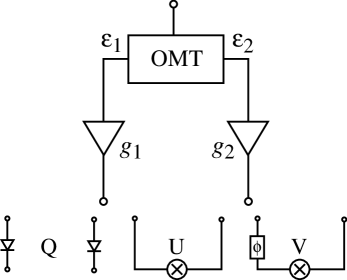
Figure 1: Block diagram for simple polarimeters. The orthomode transducer (OMT) separates two orthogonal linear polarization states with a leakage between the two characterized by $(\epsilon_{1},\epsilon_{2})$. After amplification with gain fluctuations $(g_{1},g_{2})$ the polarization state is detected by one or more of the following techniques: differencing the lines to produce $Q$, correlating the lines to produce $U$, correlating the lines with a phase shift $\phi=\pi/2$ to produce $V$. The roles of $Q$ and $V$ may be interchanged by placing a quarter-wave plate at the front end.

I.2 Instrumental Correspondence

Let us consider a few simple polarimeters that directly measure the polarized signal from a single spot on the sky (see Fig. 1; for state of the art techniques, see e.g. StaChu01 ). Here the incoming radiation is split into two, ideally orthogonal, components, $E_{1}$ and $E_{2}$ (using, for example an ortho-mode transducer or OMT). These components are possibly amplified and coupled into a detector that measures the polarization either by differencing or by correlation. Ideally the transfer matrix of the components that split and couple the radiation into the detector is proportional to the identity matrix: $\hat{\bf J}\propto{\bf I}$. In reality it contains systematic errors so that ${\hat{\bf J}}^{-1}{\bf J}\propto{\bf J}$. Let us parameterize these errors as Heietal01

$${\hat{\bf J}}^{-1}{\bf J}=\left(\begin{array}[]{cc}1+g_{1}&\epsilon_{1}e^{i\phi_{1}}\\ \epsilon_{2}e^{-i\phi_{2}}&(1+g_{2})e^{i\alpha}\end{array}\right)\,,$$ (7)

where $g_{1,2}$ are fluctuations in the gains (or, more generally, coupling efficiencies) of the two lines, $\alpha$ is the phase difference between the lines, $\epsilon_{1,2}$ express the non-orthogonality or cross-coupling between the lines, and $\phi_{1,2}$ are the phases of these couplings.

First consider the simple differencing of the time averaged intensity in the two lines $\left<E_{1}E_{1}^{*}\right>-\left<E_{2}E_{2}^{*}\right>$. This forms an estimate of $Q$ in a coordinate system attached to the instrument (e.g. Heietal01 ). Bolometer systems can be modeled with this set up, although the means of separating the two polarization states and the exact meaning of the parameters ($g_{1}$, $g_{2}$) may differ (see JonBhaBocLan02 for polarization sensitive bolometers). Under the assumption that $g_{1,2}$, $\epsilon_{1,2}$, $\alpha\ll 1$,

$$\delta Q =(g_{1}+g_{2})Q-(\epsilon_{2}\cos\phi_{2}-\epsilon_{1}\cos\phi_{1})U$$

$$\quad+(g_{1}-g_{2})\Theta\,,$$ (8)

so common-mode gain fluctuations act as a normalization error $a=(g_{1}+g_{2})$ on $Q$, the cross-couplings act as a rotation $\omega=(\epsilon_{2}\cos\phi_{2}-\epsilon_{1}\cos\phi_{1})/2$ and differential gain fluctuations leak temperature into polarization $\gamma_{1}=(g_{1}-g_{2})$.

Now consider a simple correlation polarimeter where the signal in the two lines are correlated as $\left<E_{1}E_{2}^{*}\right>$ which forms an estimate of $U$ in the instrument basis (e.g. Heietal01 ). Then the errors in the determination become

$$\delta U =(g_{1}+g_{2})U+(\epsilon_{2}\cos\phi_{2}-\epsilon_{1}\cos\phi_{1})Q$$

$$\quad+(\epsilon_{1}\cos\phi_{1}+\epsilon_{2}\cos\phi_{2})\Theta\,,$$ (9)

so again $a=(g_{1}+g_{2})$, $\omega=(\epsilon_{2}\cos\phi_{2}-\epsilon_{1}\cos\phi_{1})/2$ but leakage from $\Theta$ into $U$ is given by $\gamma_{2}=(\epsilon_{1}\cos\phi_{1}+\epsilon_{2}\cos\phi_{2})$. Instead of differential gain fluctuations, the cross-coupling between the lines is responsible for the monopole leakage in a correlation system.

Notice that under the assumption of $\alpha\ll 1$ and vanishing intrinsic $V$, the phase error $\alpha$ does not appear to first order. It is instructive to consider the case where $\alpha$ is large, say $\alpha=\pi/2$. In this case the correlation polarimeter actually measures $V$ not $U$ (see Fig. 1). In general, the phase error $\alpha$ rotates $U$ into $V$.

A complex correlation polarimeter actually takes advantage of the ($U$,$V$) rotation to measure ($Q$,$U$) simultaneously (e.g. Coretal99 ). Here, circular polarization states are coupled into the lines using, for example a quarter wave plate before the OMT. This effectively converts $Q$ into $V$ in the instrument basis. The Jones matrix of the quarter wave plate is

$${\bf J}_{1/4}(\theta)={1\over\sqrt{2}}\left(\begin{array}[]{cc}-\cos 2\theta-i&\sin 2\theta\\ \sin 2\theta&\cos 2\theta-i\end{array}\right)\,,$$ (10)

where $\theta$ gives the orientation of the plate with respect to the OMT (ideally $\theta=\pi/4$). After amplification, the signal can be coupled into two different correlators, which include different phase shifts between the lines. These additional phase shifts can be represented with the transfer function:

$${\bf J}_{\rm phase}(\phi)=\left(\begin{array}[]{cc}1&0\\ 0&e^{i\phi}\end{array}\right)\,.$$ (11)

For one correlator $\phi$ is set to zero, yielding an estimate of $U$, while the other correlator has $\phi=\pi/2$, providing an estimate of $Q$.

Now let us consider the effect of certain imperfections. Consider the actual transfer matrices of the two correlations to be

$${\bf J}_{U} ={\bf J}_{\rm line}(g_{1},g_{2},\epsilon_{1},\epsilon_{2}){\bf J}_{1/4}(\pi/4+\beta)\,,$$ (12)

$${\bf J}_{Q} ={\bf J}_{\rm phase}(\pi/2+\psi){\bf J}_{\rm line}(g_{1},g_{2},\epsilon_{1},\epsilon_{2}){\bf J}_{1/4}(\pi/4+\beta)\,,$$

and the assumed transfer matrices to be

$$\hat{\bf J}_{U} ={\bf J}_{1/4}(\pi/4)\,,$$ (13)

$$\hat{\bf J}_{Q} ={\bf J}_{\rm phase}(\pi/2){\bf J}_{1/4}(\pi/4)\,,$$

where the line matrix is taken from Eqn. (7) with the phase factors set to zero for simplicity. Then the errors become

$$\delta(Q\pm iU) =[(g_{1}+g_{2})\pm 2i\beta](Q\pm iU)$$

$$\quad+\psi\,U+(\epsilon_{1}+\epsilon_{2})\Theta\,.$$ (14)

The new feature in this system that was not present in the simple correlation polarimeter is an asymmetry between $Q$ and $U$ which is first order in the phase error $\psi$. More generally, a technique that simultaneously measures $Q$ and $U$ may have separate transfer properties (calibration, rotation, etc.) that appear as a coupling of opposite spin states $Q+iU$ and $Q-iU$. We will call such effects spin flip terms.

The Jones matrix formalism can be applied to more complicated polarimeters, such as inteferometers, or other systematics such as the finite emissivity of the dish polarimeters Far02 . In general, the systematic errors in the detector system will lead to calibration errors, rotation of linear polarization, leakage of temperature into polarization, and coupling between the two spin states $Q\pm iU$.

I.3 Map distortions

Errors in the polarization sensitivity of the detector system that vary with time will translate into errors in the polarization sky maps that vary with position. Map making generally proceeds by modeling the time ordered data as a vector of numbers ${\bf d}$ (e.g. deOetal02 )

$${\bf d}={\bf A}{\bf s}+{\bf n}\,,$$ (15)

where ${\bf n}$ is the instrumental noise and ${\bf s}$ is the model of the signal, say $\{Q(\hat{\bf n}_{1}),U(\hat{\bf n}_{1})...,Q(\hat{\bf n}_{n_{\rm p}}),U(\hat{\bf n}_{n_{\rm p}})\}$ for a sky map with $n_{\rm p}$ pixels. Here ${\bf A}$ is the pointing matrix and in its simplest incarnation just encodes the sky pixel at which the instrument is pointed at the given time. More generally the pointing matrix also encodes the beam and the chopping strategy where different pointings are differenced to remove systematic offsets. The additional complication for polarization is that the pointing matrix also has to encode the orientation of the instrument to transform $(Q,U)$ in the instrument basis to the fixed sky. This is an advantage since systematic errors like the monopole leakage $(\gamma_{1},\gamma_{2})$ are fixed to the instrument basis and not the sky.

Given the statistical properties of the noise ${\bf N}=\langle{\bf n}{\bf n}^{t}\rangle$, the minimum variance map reconstruction is

$$\hat{\bf s}=[{\bf A}^{t}{\bf N}{\bf A}]^{-1}{\bf A}^{t}{\bf N}{\bf d}\,.$$ (16)

This weighting of the data vector then also describes the transformation of the instrumental systematic errors to errors in the map. In the simplest case of white detector noise, fixed instrument orientation, simultaneous $Q$ and $U$ detection and no chopping, the weighting simply averages the $n_{\rm p}$ separate pointings for each pixel. If the systematic fields, e.g. the calibration error $a(t)$ were uncorrelated in time, they would remain so in the map but with a variance that is reduced by ${n_{\rm p}}$. Low frequency temporal correlations in the systematics will produce correlated noise in the map. This is generally controlled by spatially cross-linking the scans WriHinBen96 ; Janetal96 . A noise power of the $1/f$ form will typically lead to spatial correlations between white and $1/l$ Teg97 , where $l$ is the angular frequency or multipole moment (see §III.1). Note that even a $1/l$ spectrum gets most of its variance from high $l$ and so contamination at the pixel or beam scale will be of particular interest in §III.

Since the translation between the temporal and map domain is conceptually straightforward but highly dependent on the scanning strategy, we parameterize the systematic errors directly in the map

$$\delta[Q\pm iU](\hat{\bf n}) =[a\pm i2\omega](\hat{\bf n})[Q\pm iU](\hat{\bf n})$$

$$\quad+[f_{1}\pm if_{2}](\hat{\bf n})[Q\mp iU](\hat{\bf n})$$ (17)

$$\quad+[\gamma_{1}\pm i\gamma_{2}](\hat{\bf n})\Theta(\hat{\bf n})\,.$$

These correspond to calibration and rotation, spin-flip coupling and monopole leakage errors as they appear in the map.

II Local Contamination

In the previous section, we dealt with polarization transfer in a single, perfectly known, direction on the sky. An experiment necessarily has finite resolution and thus there is an additional class of contamination associated with the resolution or beam of the experiment. We will consider here contamination from a local coupling between the Stokes parameters which models low order anisotropy in the polarized beams.

II.1 Description

Let us consider the polarization fields to be mixed locally

$$\delta[Q\pm iU](\hat{\bf n};\sigma) =\sigma{\bf p}(\hat{\bf n})\cdot\nabla[Q\pm iU](\hat{\bf n};\sigma)$$ (18)

$$\quad+\sigma[d_{1}\pm id_{2}](\hat{\bf n})[\partial_{1}\pm i\partial_{2}]\Theta(\hat{\bf n};\sigma)$$

$$\quad+\sigma^{2}q(\hat{\bf n})[\partial_{1}\pm i\partial_{2}]^{2}\Theta(\hat{\bf n};\sigma)\,,$$

where the fields are smoothed over the average beam of the experiment, here denoted by $\sigma$, the Gaussian width. Therefore the fields ${\bf p}$, ${\bf d}$ and $q$ represent sensitivity to structure in the fields on the scale of the beam. We will call these the pointing error, dipole leakage and quadrupole leakage respectively.

We truncate the local coupling at the dipole level for the polarization and the quadrupole level for the temperature. These terms have a direct correspondence to known systematics as we shall see. More generally, the form of these couplings is dictated by the properties of the polarization field under rotation and can be generalized to higher order in a straightforward manner.

II.2 Instrumental Correspondence

Local couplings are primarily due to imperfections in the beams. Even a perfectly on-axis, azimuthally symmetric telescope will not in general produce a completely azimuthally symmetric and perfectly polarized beam. In general the beam has a finite ellipticity along the axis of polarization, and there is a “cross-polar” beam which couples to the “wrong” polarization state (additional asymmetries may appear in off-axis telescopes Heietal01 ). Both these imperfections arise because the surface normal to the optics has different orientations with respect to polarization axis depending on where the incident radiation strikes the telescope Rum66 ; Tin96 .

As an illustrative model of these effects, consider the case where the receiver on the telescope is a simple differencing polarimeter. Here the effects of the cross-polar beams are of second order, and will be ignored. Radiation from the sky is then coupled into one line of the detector through a perfectly polarized beam:

$$B(\hat{\bf n};{\bf b},e) ={1\over 2\pi\sigma^{2}(1-e^{2})}\exp\Big{[}-{1\over 2\sigma^{2}}\Big{(}{(n_{1}-b_{1})^{2}\over(1+e)^{2}}$$

$$\quad+{(n_{2}-b_{2})^{2}\over(1-e)^{2}}\Big{)}\Big{]}\,,$$ (19)

where ${\bf b}$ is the offset between the beam center and the desired direction on the sky, $\sigma$ is the mean beamwidth, and $e$ is the ellipticity Heietal01b . These parameters are different for the different polarizations, and the difference in the beams enters into the $Q$ measurement

$$B(\hat{\bf n};{\bf b}_{a},e_{a})-B(\hat{\bf n};{\bf b}_{b},e_{b})\,.$$ (20)

To first order in the sums and differences of the ellipticities and pointing errors

$$\sigma{\bf p} =({\bf b}_{a}+{\bf b}_{b})/2\,,$$

$$\sigma{\bf b}_{d} =({\bf b}_{a}-{\bf b}_{b})/2\,,$$

$$e_{s} =(e_{a}+e_{b})/2\,,$$

$$q =(e_{a}-e_{b})/2\,,$$ (21)

we obtain

$$\hat{Q}(\hat{\bf n};\sigma) =\int d\hat{\bf n}^{\prime}B(\hat{\bf n}^{\prime})\Big{\{}Q(\hat{\bf n}+\hat{\bf n}^{\prime}+\sigma{\bf p})$$

$$\quad+\Big{[}({{\bf b}_{d}\cdot{\hat{\bf n}^{\prime}}\over\sigma})+{q\over\sigma^{2}}({n_{2}^{\prime}}^{2}-{n_{1}^{\prime}}^{2})\Big{]}\Theta(\hat{\bf n}+\hat{\bf n}^{\prime})\Big{\}}\,,$$

$$\approx Q(\hat{\bf n};\sigma)+\sigma{\bf p}\cdot\nabla Q(\hat{\bf n};\sigma)+\sigma{\bf b}_{d}\cdot\nabla\Theta(\hat{\bf n};\sigma)$$

$$\quad+\sigma^{2}q[\partial_{1}^{2}-\partial_{2}^{2}]\Theta(\hat{\bf n};\sigma)\,,$$ (22)

where the average beam $B(\hat{\bf n})=B(\hat{\bf n};0,0)$ and we drop second derivative terms in $Q$. A difference in the mean beamwidth of the two beams has the same form as a contribution to the monopole leakage except that the filter for the temperature field is the beam difference not beam and is not simply a low pass filter.

A pointing offset in both beams becomes a gradient coupling in polarization and a differential beam ellipticity or “squash” becomes a coupling to the temperature quadrupole. These have a clear correspondence to the local contamination model of Eqn. (18). A differential pointing offset, or “squint” translates into coupling to the temperature dipole. The exact correspondence to the model is not precise since the leakage does not truly behave as a false polarization. For example under rotation of the instrument by $\pi$, the false $Q$ reverses sign. The model of Eqn. (18) with ${\bf d}$ referenced to the sky (not the instrument) does transform as polarization and so should be viewed as the residual dipole sensitivity after correction. The quadrupolar coupling is particularly dangerous since it behaves precisely as a polarization and cannot be removed through rotation of the instrument. For example, even a circularly symmetric temperature hot spot becomes a radial pattern of polarization through its local quadrupole moment.

These leakage terms also appear if the receiver is a correlation polarimeter. In this case, the leakage from temperature to polarization is due to the amplitude and shape of the cross-polar beam instead of asymmetries in the main beam Heietal01 . However, because both of these imperfections have a common origin in the variations in the boundary conditions at optical surfaces, it turns out that a differencing system or a correlation polarimeter will obtain similar leakage terms due to the local effects (after accounting for the orientation of the receiver with respect to the optics) Nap89 ; Zha93 . Interferometric polarimeters have related effects on the scale of the primary beam although some of the implications for $B$-modes will differ since the measured modes are below the beam scale Leietal02 .

If stable, these effects can be removed given a beam measurement and the true temperature field on the sky using the formalism of anisotropic polarized beams Chaetal00 ; FosDorBou02 . Moreover, as the circularly symmetric hot spot example implies, a stable quadrupole leakage produces no $B$-mode in the polarization map (see §III.2). It is the instability in these effects or errors in the subtraction that appear as errors in the map.

III B-mode Contamination

We study here the implications of polarization transfer and local contamination on the $B$-modes of the polarization. In §III.1, we give the harmonic representation of the polarization and contamination fields. In §III.2, we compute the contamination to the $B$ power spectrum from polarization distortion and temperature leakage. We explore the implications of these effects in §III.3.

III.1 Field Representation

The polarization and contamination fields may in general be decomposed into harmonics appropriate to their properties under rotation or spin. For small sections of the sky, these harmonics are simply plane waves Sel97 ; WhiCarDraHol99 ; in the Appendix we treat the general all-sky case. We will follow the convention that a complex field $S$ of spin $\pm s$ is decomposed as

$$[S_{1}\pm iS_{2}](\hat{\bf n}) =(\mp 1)^{s}\int{d^{2}l\over(2\pi)^{2}}[S_{a}\pm iS_{b}]({\bf l})e^{\pm is\phi_{l}}\,,$$ (23)

where $\cos\phi_{l}=l_{x}/l$. The complex polarization $Q\pm iU$ is a spin $\pm 2$ field and we will follow the conventional nomenclature that its harmonics are named $E\pm iB$. This property requires the calibration $a$, rotation $\omega$, and quadrupole leakage to be spin-0 fields, the pointing $p_{1}\pm ip_{2}$ and dipole leakage $d_{1}\pm id_{2}$ to be $\pm 1$ fields, the monopole leakage $\gamma_{1}\pm i\gamma_{2}$ to be $\pm 2$ fields, and the spin-flip $f_{1}\pm if_{2}$ to be $\pm 4$ fields. For spin $\pm 1$ fields $S_{a}$ is the divergence-free part and $S_{b}$ is the curl-free part.

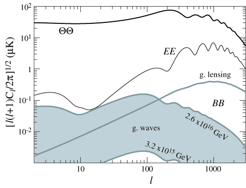
Figure 2: Scalar CMB power spectra in temperature ($\Theta\Theta$) and $E$-mode polarization ($EE$) compared with $B$-mode polarization due to gravitational lensing and gravitational waves at the maximum allowable $2.6\times 10^{16}$ GeV WanTegZal02 and minimum detectable $3.2\times 10^{15}$ GeV level KnoSon02 . The $\Lambda$CDM model shown has parameters given in III.1.

Under the assumption of statistical isotropy of the fields, their two point correlations are defined by their (cross) power spectra

$$\left<S({\bf l})^{*}S^{\prime}({\bf l}^{\prime})\right>=(2\pi)^{2}\delta({\bf l}-{\bf l}^{\prime})C_{l}^{SS^{\prime}}\,,$$ (24)

where $S$, $S^{\prime}$ are any of the fields. In particular, the CMB polarization is described by $C_{l}^{EE}$ and $C_{l}^{BB}$ and CMB temperature by $C_{l}^{\Theta\Theta}$. Note that $C_{l}^{BB}=0$ for scalar fluctuations in linear theory. For definiteness, let us take as a fiducial model: a baryon density of $\Omega_{b}h^{2}=0.02$, cold dark matter density of $\Omega_{c}h^{2}=0.128$, a cosmological constant of $\Omega_{\Lambda}=0.65$, reionization optical depth $\tau=0.05$, an initial amplitude of comoving curvature fluctuations of $\delta_{\zeta}=4.79\times 10^{-5}$ (Hu01c or $\sigma_{8}=0.92$), and a scalar spectral index of $n=1$ in a spatially flat universe. Power spectra for the fiducial model are shown in Fig. 2. It is the large range in expected signals that make the contamination problem for $BB$ so problematic.

We will calculate the contamination to the $B$-mode polarization power spectrum assuming no intrinsic $B$-modes and generally will plot

$$\Delta B\equiv\left({l(l+1)\over 2\pi}C_{l}^{BB}\right)^{1/2}\,,$$ (25)

in units of $\mu$K. The general case is given in the Appendix.

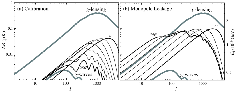
Figure 3: Coherence dependence of $B$-mode contamination (a) for calibration $a$ with rms $A_{a}=10^{-2}$ (b) for monopole-leakage $\gamma_{a}$, $\gamma_{b}$ with $A_{\gamma_{a}}=A_{\gamma_{b}}=10^{-3}$ added in quadrature. The beam scale is FWHM = $(8\ln 2)^{1/2}\sigma=1^{\prime}$ to remove beam effects and the FWHM coherence $(8\ln 2)^{1/2}\alpha$ is stepped from $256^{\prime}$ to $4^{\prime}$ in factors of 2. Other effects follow the trend of calibration errors not monopole leakage. For a coherence large compared with the CMB acoustic peaks, $B$ contamination picks up their underlying structure. Here and in the following figures, the gravitational lensing and minimum detectable gravitational wave ($E_{i}=3.2\times 10^{15}$GeV) $B$-modes are shown for reference (thick shaded lines). The scaling with $E_{i}$ of the peak in the $B$-mode spectrum is shown on the right hand axis.

Although the distortion fields need not be statistically isotropic, for illustrative purposes we will take contamination fields with power spectra of the form

$$C_{l}^{SS}\propto\exp(-l(l+1)\alpha_{S}^{2}),$$ (26)

i.e. white noise above some coherence scale $\alpha_{S}$. The normalization constant is set so that

$$A_{S}^{2}=\int{d^{2}l\over(2\pi)^{2}}C_{l}^{SS}\,,$$ (27)

The set ($A_{S}$,$\alpha_{S}$) then characterizes the rms and coherence of the contamination field.

III.2 $B$-modes

The changes to the $B$-mode harmonics due to the calibration, rotation, spin-flip and pointing take the form

$$\delta B({\bf l})=\int{d^{2}l_{1}\over(2\pi)^{2}}S({\bf l}_{1})E({\bf l}_{2})W_{S}({\bf l}_{1},{\bf l}_{2})\,,$$ (28)

with ${\bf l}_{2}={\bf l}-{\bf l}_{1}$ and

$$W_{a} =\sin[2(\phi_{l_{2}}-\phi_{l})]\,,$$

$$W_{\omega} =2\cos[2(\phi_{l_{2}}-\phi_{l})]\,,$$

$$W_{p_{a}} =\sigma({\bf l}_{2}\times\hat{\bf l}_{1})\cdot\hat{\bf z}\sin[2(\phi_{l_{2}}-\phi_{l})]\,,$$

$$W_{p_{b}} =\sigma({\bf l}_{2}\cdot\hat{\bf l}_{1})\sin[2(\phi_{l_{2}}-\phi_{l})]\,,$$

$$W_{f_{a}} =\sin[2(2\phi_{l_{1}}-\phi_{l_{2}}-\phi_{l})]\,,$$

$$W_{f_{b}} =\cos[2(2\phi_{l_{1}}-\phi_{l_{2}}-\phi_{l})]\,,$$ (29)

for the various effects. Here ${{\bf l}_{1}}=l_{1}\hat{\bf l}_{1}$. These relations imply contamination to the $BB$ power spectrum of

$$\delta C_{l}^{BB}=\sum_{SS^{\prime}}\int{d^{2}l_{1}\over(2\pi)^{2}}C_{l_{1}}^{SS^{\prime}}C_{l_{2}}^{EE}(\sigma)W_{S}^{*}W_{S^{\prime}}\,,$$ (30)

where

$$C_{l}^{EE}(\sigma)=C_{l}^{EE}\exp(-l(l+1)\sigma)$$ (31)

is the $EE$ power spectrum smoothed over the average beam.

Similarly the change due to temperature leakage can be described by

$$\delta B({\bf l})=\int{d^{2}l_{1}\over(2\pi)^{2}}S({\bf l}_{1})\Theta({\bf l}_{2})W_{S}({\bf l}_{1},{\bf l}_{2})\,,$$ (32)

with

$$W_{\gamma_{a}} =\sin[2(\phi_{l_{1}}-\phi_{l})]\,,$$

$$W_{\gamma_{b}} =\cos[2(\phi_{l_{1}}-\phi_{l})]\,,$$

$$W_{d_{a}} =-(l_{2}\sigma)\cos[\phi_{l_{1}}+\phi_{l_{2}}-2\phi_{l}]\,,$$

$$W_{d_{b}} =(l_{2}\sigma)\sin[\phi_{l_{1}}+\phi_{l_{2}}-2\phi_{l}]\,,$$

$$W_{q} =-(l_{2}\sigma)^{2}\sin[2(\phi_{l_{2}}-\phi_{l})]\,,$$ (33)

leading to

$$\delta C_{l}^{BB}=\sum_{SS^{\prime}}\int{d^{2}l_{1}\over(2\pi)^{2}}C_{l_{1}}^{SS^{\prime}}C_{l_{2}}^{\Theta\Theta}(\sigma)W_{S}^{*}W_{S^{\prime}}\,,$$ (34)

for the power spectrum contamination Additional .

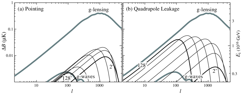
Figure 4: Beam dependence of $B$-mode contamination for (a) pointing with an rms $A_{p_{a}}=A_{p_{b}}=10^{-2}$ (in units of the Gaussian beam width) added in quadrature (b) quadrupole leakage with an rms $A_{q}=0.002$ (in units of differential beam ellipticity). The coherence $\alpha$ is set to max($\sigma$, $10^{\prime}/(8\ln 2)^{1/2}$) and the beam is stepped from $128^{\prime}$ to $2^{\prime}$ in factors of 2.

A few limiting cases are worth noting before proceeding to specific examples. If $l_{1}\gg l$ as is the case for power in the contamination field at much smaller scales than the $l$ of interest, $l_{1}\approx l_{2}$ and $\phi_{1}\approx-\phi_{2}$. The geometric factors in Eqn. (29) and (33) cause all effects to efficiently produce $B$-modes except the pointing curl $p_{a}$ where the cross product vanishes. In the opposite limit $l_{1}\ll l$ then $l_{2}\approx l$ and $\phi_{2}\approx\phi$. Here the calibration $a$, pointing terms, and quadrupole leakage are geometrically suppressed. The reason is clear from the nature of the effects: a uniform distortion in any of these quantities does not produce a $B$-mode.

III.3 Scientific Impact

Cosmological $B$-modes come from two main sources: gravitational waves, also known as tensor perturbations, KamKosSte97 ; ZalSel97 and gravitational lensing of polarization by the large-scale structure of the universe ZalSel98 . Aside from small but interesting effects due to the dark energy, reionization and massive neutrinos, the gravitational lensing $B$-modes can be predicted given parameters extracted from the CMB temperature spectrum. The gravitational lensing prediction in the fiducial model is shown in Figs. 2-5 as the shaded top line.

Under slow-roll inflation, the initial amplitude of the gravitational wave spectrum is parameterized by the energy scale of inflation $E_{i}$ and its spectrum is nearly scale invariant. It predicts a $B$-mode power spectrum amplitude with a peak at $l\approx 90$ of TS

$$\Delta B_{\rm peak} =0.024\left({E_{i}\over 10^{16}{\rm GeV}}\right)^{2}\mu{\rm K}\,.$$ (35)

Under reasonable cosmological assumptions, the CMB temperature anisotropies constrain the energy scale to be $E_{i}<2.6\times 10^{16}$GeV WanTegZal02 . If the energy scale is less than $E_{i}<3.2\times 10^{15}$GeV, then even with a direct reconstruction of the lensing signal HuOka02 , a significant detection of the inflationary $B$-modes cannot be achieved KnoSon02 . These two extremes are shown in Fig. 2 and are used in Figs. 3-5, to mark the range across which the systematic errors need to be controlled. We will take the prediction for the middle of this range ($E_{i}=10^{16}$ GeV) as the minimal level that a next generation polarization mission must reduce errors. For reference, with no systematics or foregrounds the Planck satellite planck can in principle achieve a 1$\sigma$ bound of $E_{i}=1.1\times 10^{16}$ GeV Hu01c .

Given that the inflationary $B$-modes peak at $l\approx 90$, one might naively assume that only contamination fields with coherence corresponding to degree scales would be problematic. However because equations (28) and (32) represent mode coupling, this expectation is incorrect. The problem is that the intrinsic power in the CMB polarization fields as well as the temperature gradient and second derivative fields peak on the scale associated with the diffusion scale at recombination, now observationally determined to be $l\approx 10^{3}$ or $10^{\prime}$ by the CBI experiment Peaetal02 . In Fig. 3a, we show the effect of a calibration error with the same rms $A_{a}=10^{-2}$ but different coherence scales $\alpha_{a}$. For coherence scales above $(8\ln 2)^{1/2}\alpha_{a}=10^{\prime}$, the contamination actually increases as the coherence scale decreases. For most effects, the coherence scale that gives the maximum total contamination is the larger of the beam scale and $\sim 10^{\prime}$. The mathematical reason is that the mode coupling sets ${\bf l}={\bf l}_{1}+{\bf l}_{2}$ which forms a triangle with sides $(l,l_{1},l_{2})$. For CMB power at ${\bf l}_{2}\gg{\bf l}$ contamination power at $l_{1}\approx l_{2}$ causes most of the leakage by forming a flattened triangle.

The exception is the monopole leakage which takes power out of the CMB temperature power spectrum itself, not derivative power spectra which are weighted by factors of $l$. Here the most damaging coherence scale is associated with the first peak in the CMB at $l\approx 200$ (see Fig. 2) which is dangerously close to the $l\sim 100$ scale of interest for gravitational waves. Fig. 3b illustrates this problem and shows that degree scale fluctuations in monopole leakage from low frequency noise must be controlled to substantially better than $10^{-3}$ rms for $E_{i}<10^{16}$GeV.

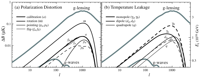
Figure 5: All effects for a beam and coherence of FWHM = $(8\ln 2)^{1/2}\sigma=10^{\prime}$. (a) Polarization distortion for an rms of $A=10^{-2}$ from calibration $a$, rotation $\omega$ ($0.6^{\circ}$ rms), pointing ($p_{a}$,$p_{b}$) ($2.5^{\prime\prime}$ rms) , and spin flip ($f_{a}$,$f_{b}$). (b) Temperature leakage for an rms of $A=10^{-3}$ from monopole ($\gamma_{a}$,$\gamma_{b}$), dipole ($d_{a}$,$d_{b}$) and quadrupole ($q$) terms. The “$b$” component of each effect is shown with dashed lines.

Pointing, dipole and quadrupole leakage errors are expressed in terms of fractions of the beam and hence can depend strongly on the beam scale. The contamination at $l\approx 90$ from pointing errors of a fixed fraction of the beam holds roughly constant for beam sizes above a FWHM $\approx 10^{\prime}$. At this point most of the structure in the underlying CMB fields become resolved and the contamination depends on the absolute pointing error relative to the CMB $10^{\prime}$ coherence (see Fig. 4). Pointing problems must be constrained to better than the larger of $10^{-1}$ of the Gaussian beamwidth or $15^{\prime\prime}$ absolute rms for $E_{i}<10^{16}$GeV and must reach $10^{-2}$ of the beamwidth or $1.5^{\prime\prime}$ absolute to be safely irrelevant.

The quadrupole leakage provides a more extreme example. Contamination for a fixed rms differential ellipticity strongly increases with increasing beam and so a beam $<10^{\prime}$ FWHM greatly reduces the contamination. The dipole leakage lies in between these two cases in sensitivity to the beam scale. In Fig. 5 we show all of the effects, for a choice of beam and coherence of FWHM $=10^{\prime}$ and an rms of $10^{-2}$ for polarization distortions and $10^{-3}$ for temperature leakage.

It is useful to have an approximate scaling for the rms amplitude of the systematic needed to make the contamination on the same level (at $l=90$) as a given target inflationary energy scale. Let us approximate the rms as a power law in the FWHM of the beam

$$A_{S}=C_{S}\left({E_{i}\over 10^{16}{\rm GeV}}\right)^{2}({\rm FWHM\over 10^{\prime}})^{p_{S}}\,.$$ (36)

In Table 1, we give the coefficients $C_{S}$ and $p_{S}$ for two choices of the coherence scale: $\alpha_{S}=\sigma$ and $(8\ln 2)^{1/2}\alpha_{S}=2^{\circ}$. The beam dependence is calculated locally around $10^{\prime}$ and should not be used to extrapolate results far from this.

Type	$C_{S}$ ($\sigma$)	$p_{S}$ ($\sigma$)		$C_{S}$ ($2^{\circ}$)	$p_{S}$ ($2^{\circ}$)
Calibration $a$	0.060	-0.3		0.049	0.0
Rotation $w$	0.015	-0.3		0.011	0.0
Pointing $p_{a}$	0.75	-1.3		0.53	-1.0
Pointing $p_{b}$	0.098	-0.7		0.57	-1.0
Flip $f_{a}$	0.061	-0.3		0.046	0.0
Flip $f_{b}$	0.059	-0.3		0.045	0.0
Monopole $\gamma_{a}$	0.0023	-0.9		0.0006	0.0
Monopole $\gamma_{b}$	0.0019	-0.9		0.0005	0.0
Dipole $d_{a}$	0.0077	-1.3		0.0053	-1.0
Dipole $d_{b}$	0.0077	-1.3		0.0056	-1.0
Quadrupole $q$	0.0124	-1.5		0.0394	-2.0

Table 1: Scaling parameters for contamination effects with a coherence of the beam scale $\sigma$ and $2^{\circ}$. $C_{S}$ represents the minimum rms required to not exceed a signal at $E_{i}=10^{16}$ GeV; the ultimate limit of $3.2\times 10^{15}$ GeV would require an order of magnitude smaller rms.

IV Discussion

We have provided a fairly general description of the phenomenology of systematic errors that can occur in polarization maps, their correspondence with known classes of instrumental problems, and their impact on the science of $B$-modes. Instability in the systematic effects or errors in their removal lead to residual contamination in the polarization maps that are parameterized by 7 fields, 4 of which have two components each, for a total of 11 distortion parameters per position on the sky or multipole moment. These errors are associated with calibration, rotation, pointing (2), spin flip (2), monopole leakage (2), dipole leakage (2) and quadrupole leakage. The three temperature leakage effects are named for the type of temperature fluctuation across the beam scale that they respond to and are especially dangerous due to the extremely low level of polarization expected in the $B$-modes. Monopole leakage generally arises in the receiver; dipole and quadrupole leakage are associated with asymmetries in the beam.

We have illustrated these problems by modelling the fluctuations in these contamination fields with an rms amplitude and coherence. In general, it is not sufficient to control the fluctuations in the field on the degree scales of interest for gravitational wave $B$-modes. Because all of these effects transfer power from the CMB fluctuations themselves, the most dangerous fluctuations are those that are on the same scale as most of the power in the CMB fields. For all but the monopole leakage effect, which can draw power out of the first acoustic peak, the underlying power lies at the diffusion damping scale of $l\sim 10^{3}$ or $\sim 10^{\prime}$. Unless the beam resolves this scale, even uncorrelated white noise fluctuations in the fields can substantially contaminate low multipoles in $B$.

The interplay between the beam scale and $10^{\prime}$ coherence scale of the CMB fields plays an especially important role in pointing, dipole leakage and quadrupole leakage. These problems couple local derivatives of the CMB fields into false polarization signals. They can largely be eliminated if the beam is sufficiently small so that the CMB fields are smooth across the beam scale. Small beams are also desirable for constructing weak lensing mass maps from the $B$-mode polarization HuOka02 .

Based on the systematic errors of the current generation of experiments, these problems should be challenging but not insurmountable. The DASI instrument had percent level monopole leakage which was stable at the fractional percent level and quadrupole leakage also at the percent level which was highly stable. It also had rotational uncertainties at the percent level Leietal02 . The PIQUE instrument had a monople leakage at under the percent level and a dipole leakage at less than 2.5% Hed02 . The polarization sensitive bolometers for the upcoming Boomerang experiment JonBhaBocLan02 and planned for Planck have monopole leakage at the percent level but are claimed to be very stable.

This exploratory study of polarization effects should help to provide some rough guidance on the long road ahead toward the ultimate goal of detecting the gravitational waves from inflation.

Acknowledgments: We thank Stephan Meyer for guidance; Scott Dodelson, John Kovac, Clem Pryke, Bruce Winstein and the CfCP CMB Working Group for many stimulating discussions. WH is supported by NASA NAG5-10840 and the DOE OJI program; MMH by the CfCP under NSF PHY 0114422, and MZ by NSF grants AST 0098606 and PHY 0116590 and by the David and Lucille Packard Foundation Fellowship for Science and Engineering.

Appendix A General Treatment

The flat sky expansion in Eqn. (23) may be generalized by decomposing the fields as ZalSel98

$$[S_{1}\pm iS_{2}](\hat{\bf n}) =(i)^{s}\sum_{lm}[S_{a}\pm iS_{b}]_{lm}\,{\vphantom{Y}}_{\pm s}Y_{lm}(\hat{\bf n})\,,$$

where $\,{\vphantom{Y}}_{s}Y_{lm}$ is the spin-$s$ spherical harmonic spin .

The corrections to the $E$ and $B$ harmonics of the polarization from the distortion field $S$ can be generally expressed as

$$\delta X_{lm}^{\pm} =(-1)^{m}\sum_{l_{1}m_{1}}\sum_{l_{2}m_{2}}\sqrt{(2l+1)(2l_{1}+1)(2l_{2}+1)\over 4\pi}$$ (37)

$$\quad\times\left(\begin{array}[]{ccc}\!l\!&l_{1}\!&l_{2}\!\\ \!-m\!&m_{1}\!&m_{2}\!\end{array}\right)S_{l_{1}m_{1}}L_{S}$$ (40)

$$\quad\times a_{S}^{\pm}(e_{S}^{+}X_{l_{2}m_{2}}^{\pm}+e_{S}^{-}X_{l_{2}m_{2}}^{\mp})\,,$$

where $X^{+}\equiv E$, $X^{-}\equiv iB$ and $S\in a,\omega,p_{a},p_{b},f_{a},f_{b}$ and

$$e^{\pm}_{a,p_{b}} ={1\over 2}\left[1\pm(-1)^{l+l_{1}+l_{2}}\right],$$

$$e^{\pm}_{\omega,p_{a}} ={1\over 2}\left[1\mp(-1)^{l+l_{1}+l_{2}}\right],$$

$$e^{\pm}_{f_{a}} =\pm{1\over 2}\left[1\pm(-1)^{l+l_{1}+l_{2}}\right],$$

$$e^{\pm}_{f_{b}} =\pm{1\over 2}\left[1\mp(-1)^{l+l_{1}+l_{2}}\right],$$ (41)

selects out even and odd sums of the $l$’s. The factor $a_{S}^{\pm}=1$ for $S\in a,\omega,p_{a},p_{b}$ and $=\pm 1$ for $S\in f_{a},f_{b}$ and adjusts the relative sign.

The specific linear source terms are

$$L_{a} =-{i\over 2}L_{\omega}=\left(\begin{array}[]{ccc}\!l\!&l_{1}\!&l_{2}\!\\ \!-2\!&0\!&2\!\end{array}\right)\,,$$ (44)

$$L_{p_{b}} ={1\over 2}\Big{[}\sqrt{(l_{2}+2)(l_{2}-1)}\left(\begin{array}[]{ccc}\!l\!&l_{1}\!&l_{2}\!\\ \!-2\!&1\!&1\!\end{array}\right)$$ (47)

$$\quad+\sqrt{(l_{2}-2)(l_{2}+3)}\left(\begin{array}[]{ccc}\!l\!&l_{1}\!&l_{2}\!\\ \!-2\!&-1\!&3\!\end{array}\right)\Big{]}\,,$$ (50)

$$L_{p_{a}} ={-i\over 2}\Big{[}\sqrt{(l_{2}+2)(l_{2}-1)}\left(\begin{array}[]{ccc}\!l\!&l_{1}\!&l_{2}\!\\ \!-2\!&1\!&1\!\end{array}\right)$$ (53)

$$\quad-\sqrt{(l_{2}-2)(l_{2}+3)}\left(\begin{array}[]{ccc}\!l\!&l_{1}\!&l_{2}\!\\ \!-2\!&-1\!&3\!\end{array}\right)\Big{]}\,,$$ (56)

$$L_{f_{a}} =-iL_{f_{b}}=\left(\begin{array}[]{ccc}\!l\!&l_{1}\!&l_{2}\!\\ \!-2\!&4\!&-2\!\end{array}\right)\,.$$ (59)

Under the assumption of statistical isotropy of the distortion fields, the perturbation to the power spectra are given by

$$\delta C_{l}^{EE} ={a_{00}\over\sqrt{4\pi}}C_{l}^{EE}+\sum_{l_{1}l_{2}SS^{\prime}}{(2l_{1}+1)(2l_{2}+1)\over 4\pi}C_{l_{1}}^{SS^{\prime}}$$

$$\quad\times a_{S}^{+}a_{S^{\prime}}^{+}[C_{l_{2}}^{EE}e^{+}_{S}e^{+}_{S^{\prime}}+C_{l_{2}}^{BB}e^{-}_{S}e^{-}_{S^{\prime}}]L_{S}^{*}L_{S^{\prime}}\,,$$

$$\delta C_{l}^{BB} ={a_{00}\over\sqrt{4\pi}}C_{l}^{BB}+\sum_{l_{1}l_{2}SS^{\prime}}{(2l_{1}+1)(2l_{2}+1)\over 4\pi}C_{l_{1}}^{SS^{\prime}}$$

$$\quad\times a_{S}^{-}a_{S^{\prime}}^{-}[C_{l_{2}}^{EE}e^{-}_{S}e^{-}_{S^{\prime}}+C_{l_{2}}^{BB}e^{+}_{S}e^{+}_{S^{\prime}}]L_{S}^{*}L_{S^{\prime}}\,,$$

$$\delta C_{l}^{EB} ={2\omega_{00}\over\sqrt{4\pi}}(C_{l}^{EE}-C_{l}^{BB})$$ (60)

$$\quad+\sum_{l_{1}l_{2}SS^{\prime}}{(2l_{1}+1)(2l_{2}+1)\over 4\pi}C_{l_{1}}^{SS^{\prime}}$$

$$\quad\times a_{S}^{+}a_{S^{\prime}}^{-}[C_{l_{2}}^{EE}e^{+}_{S}e^{-}_{S^{\prime}}+C_{l_{2}}^{BB}e^{-}_{S}e^{+}_{S^{\prime}}](-i)L_{S}^{*}L_{S^{\prime}}\,,$$

where we have allowed for the possibility of a monopole term in the calibration $a$ and rotation $\omega$. Such terms often arise from second order terms in an expansion and comes about through the variance of a distortion field across the sky. They must be kept since the net change to the power spectrum is itself second order and often cancel the linear effects. For example, second order terms in the pointing errors appear as a monopole calibration error. Since these terms do not transfer power in $EE$ to $BB$, they are not relevant for the discussion in the main paper.

Temperature leakage terms may similarly be described in their effect on $E$ and $iB$

$$\delta X_{lm}^{\pm} =(-1)^{m}\sum_{l_{1}m_{1}}\sum_{l_{2}m_{2}}\sqrt{(2l+1)(2l_{1}+1)(2l_{2}+1)\over 4\pi}$$ (61)

$$\quad\times\left(\begin{array}[]{ccc}\!l\!&l_{1}\!&l_{2}\!\\ \!-m\!&m_{1}\!&m_{2}\!\end{array}\right)S_{l_{1}m_{1}}\Theta_{l_{2}m_{2}}e_{S}^{\pm}L_{S}\,,$$ (64)

for $S\in\gamma_{a},\gamma_{b},d_{a},d_{b},q$

$$e^{\pm}_{\gamma_{a},d_{b},q} ={1\over 2}\left[1\pm(-1)^{l+l_{1}+l_{2}}\right],$$

$$e^{\pm}_{\gamma_{b},d_{a}} ={1\over 2}\left[1\mp(-1)^{l+l_{1}+l_{2}}\right],$$ (65)

and

$$L_{\gamma_{a}} =-iL_{\gamma_{b}}=\left(\begin{array}[]{ccc}\!l\!&l_{1}\!&l_{2}\!\\ \!-2\!&2\!&0\!\end{array}\right)\,,$$ (68)

$$L_{d_{b}} =iL_{d_{a}}=\sqrt{l_{2}(l_{2}+1)}\sigma\left(\begin{array}[]{ccc}\!l\!&l_{1}\!&l_{2}\!\\ \!-2\!&1\!&1\!\end{array}\right)\,,$$ (71)

$$L_{q} =-\sqrt{(l+2)!\over(l-2)!}\sigma^{2}\left(\begin{array}[]{ccc}\!l\!&l_{1}\!&l_{2}\!\\ \!-2\!&2\!&0\!\end{array}\right)\,.$$ (74)

The perturbation to the power spectra are given by

$$\delta C_{l}^{EE} =\sum_{l_{1}l_{2}SS^{\prime}}{(2l_{1}+1)(2l_{2}+1)\over 4\pi}C_{l_{1}}^{SS^{\prime}}C_{l_{2}}^{\Theta\Theta}$$

$$\quad e^{+}_{S}e^{+}_{S^{\prime}}L_{S}^{*}L_{S^{\prime}}\,,$$

$$\delta C_{l}^{BB} =\sum_{l_{1}l_{2}SS^{\prime}}{(2l_{1}+1)(2l_{2}+1)\over 4\pi}C_{l_{1}}^{SS^{\prime}}C_{l_{2}}^{\Theta\Theta}$$ (75)

$$\quad e^{-}_{S}e^{-}_{S^{\prime}}L_{S}^{*}L_{S^{\prime}}\,,$$

$$\delta C_{l}^{EB} =\sum_{l_{1}l_{2}SS^{\prime}}{(2l_{1}+1)(2l_{2}+1)\over 4\pi}C_{l_{1}}^{SS^{\prime}}C_{l_{2}}^{\Theta\Theta}$$

$$\quad e^{+}_{S}e^{-}_{S^{\prime}}(-i)L_{S}^{*}L_{S^{\prime}}\,.$$

This completes the general description of the polarization contamination from the class of map distortions considered.

References

- (1)
- (2) J. Kovac, et al. Astrophys. J, submitted astro-ph/0209478 (2002).
- (3) M. Kamionkowski, A. Kosowsky, A. Stebbins, Phys. Rev. D, 55 7368 (1997).
- (4) M. Zaldarriaga, U. Seljak, Phys. Rev. D, 55 1830 (1997).
- (5) M. Zaldarriaga, U. Seljak, Phys. Rev. D, 58 023003 (1998).
- (6) K. Benabed, F. Bernardeau, L. van Waerbeke, Phys. Rev. D, 63 043501 (2001).
- (7) W. Hu, T. Okamoto, Astrophys. J, 574 566 (2002).
- (8) A.H. Jaffe, M. Kamionkowski, L. Wang, Phys. Rev. D, 61 083501 (2000).
- (9) M. Tegmark, D.J. Eisenstein, W. Hu, A. de Oliviera Costa, Astrophys. J, 530 133 (2000).
- (10) S. Prunet, S.K. Sethi, F.R. Bouchet, Mon. Not. Roy. Astr. Soc., 314 348 (2000).
- (11) C. Baccigalupi, et al. Mon. Not. Roy. Astr. Soc., submitted astro-ph/0209591 (2002).
- (12) A. Lewis, A. Challinor, N. Turok, Phys. Rev. D, in press (2001).
- (13) E.F. Bunn, M. Zaldarriaga, M. Tegmark, A. de Oliveira-Costa, Astrophys. J, submitted astro-ph/0207338 (2002).
- (14) J. Tinbergen, Astronomical Polarimetry (Cambridge University Press, New York 1996)
- (15) C. O’Dell, PhD Thesis, U. Wisconsin astro-ph/0201224 (2002).
- (16) C. Heiles, et al. Proc. Astr. Soc. Pac., 113 1274 (2001).
- (17) S. Staggs, S. Church, Snowmass, astro-ph/0111576 (2001).
- (18) W.C. Jones, R.S. Bhatia, J.J. Bock, A.E. Lange, SPIE Proceedings, Waikaloa astro-ph/0209132 (2002).
- (19) S. Cortiglioni, et al. preprint, astro-ph/9901362 (1999).
- (20) P.C. Farese, PhD Thesis, U.C. Santa Barbara (2002).
- (21) A. de Oliveira-Costa, et al. Astrophys. J, in press astro-ph/0204021 (2002).
- (22) E.L. Wright, G. Hinshaw, C.L. Bennett, Astrophys. J, 458 53 (1996).
- (23) M. Janssen, et al. preprint, astro-ph/09602009 (1996).
- (24) M. Tegmark, Phys. Rev. D, 56 4514 (1997).
- (25) P.J. Napier in Synthesis Imaging in Radio Astronomy, edited by. R.A Perley, F.R. Schwab, A.H. Bridle (Astronomical Society of the Pacific, San Francisco 1989) p. 39
- (26) V.H. Rumsey, IEEE Transactions on Antennas and Propagation, 14 656 (1966).
- (27) C. Heiles, et al. Proc. Astr. Soc. Pac., 113 1247 (2001).
- (28) X. Zhang, IEEE Transactions on Microwave Theory and Techniques, 41 1263 (1993).
- (29) E.M. Leitch, et al. Astrophys. J, submitted astro-ph/0209476 (2002).
- (30) A. Challinor, et al. Phys. Rev. D, 62 123002 (2000).
- (31) P. Fosalba, O. Dore, F.R. Bouchet, Phys. Rev. D, 65 063003 (2002).
- (32) U. Seljak, Astrophys. J, 482 6 (1997).
- (33) M. White, J.E. Carlstrom, M. Dragovan, W.L. Holzapfel, Astrophys. J, 514 12 (1999).
- (34) W. Hu, Phys. Rev. D, 65 023003 (2002).
- (35) Cross correlation between distortion and leakage effects can lead to -power through the intrinsic temperature- polarization cross correlation . The expressions can be readily generalized to this case. Also, though we take the filtered power spectrum to be smoothed by the main beam, this description can incorporate differential beam size fluctuations in the polarized beams by simply changing the filter (see II.2).
- (36) For the scalar amplitude and parameters of the fiducial model ( or ) the ratio of quadrupolar power in CMB temperature anisotropies is .
- (37) X. Wang, M. Tegmark, M. Zaldarriaga, Phys. Rev. D, 65 123001 (2002).
- (38) L. Knox, Y.S. Song, Phys. Rev. Lett., 89 011303 (2002).
- (39) http://astro.estec.esa.nl/Planck
- (40) T.J. Pearson, et al. Astrophys. J, submitted astro-ph/0205388 (2002).
- (41) M. Hedman, PhD Thesis, Princeton University (2001); M. Hedman, et al. Astrophys. J, 573 73 (2002).
- (42) E. Newman, R. Penrose, J. Math Phys. 7, 863 (1966); J.N. Goldberg et al., ibid, 8, 2155 (1967).