Probing the extended emission-line region in 3C 171 with high-frequency radio polarimetry

Abstract

I present high-frequency polarimetric radio observations of the radio galaxy 3C 171, in which depolarization is associated with an extended emission-line region. The radio hotspots, known to be depolarized at low radio frequencies, become significantly polarized above (observer’s-frame) frequencies of 15 GHz. There is some evidence that some of the Faraday rotation structure associated with the emission-line regions is being resolved at the highest resolutions (0.1 arcsec, or 400 pc); however, the majority remains unresolved. Using the new radio data and a simple model for the nature of the depolarizing screen, it is possible to place some constraints on the nature of the medium responsible for the depolarization. I argue that it is most likely that the depolarization is due not to the emission-line material itself but to a second, less dense, hot phase of the shocked ISM, and derive some limits on its density and temperature.

1 Introduction

Extended emission-line regions (EELR) around radio galaxies are common, and often aligned with the axes of the extended radio emission (e.g. McCarthy et al. 1987; McCarthy 1993; McCarthy, Baum & Spinrad 1996). There is considerable debate as to whether EELR are ionized by photons from the nucleus or by shocks driven by the jets (e.g. Tadhunter et al. 1998). Most EELR around low-redshift sources can adequately be described by central-illumination models, while sources which show evidence for shock ionization (such as extreme emission-line kinematics) are largely at high redshift. However, there is evidence that a small minority of low-redshift radio galaxies are also more adequately described by a shock-ionization model. If the ionization is due to shocks, the physical conditions in and kinematics of the EELR may give us important information about the energetics of the radio source as a whole.

One good candidate low-redshift shock-ionization source is 3C 171, an unusual $z=0.2384$ radio galaxy. Its large-scale radio structure has been well studied (Heckman, van Breugel & Miley 1984; Blundell 1996). In its inner regions it is similar to a normal FRII, but low-surface-brightness plumes instead of normal lobes extend north and south from the hotspots. High-resolution images show knotty jets connecting the radio core with the hotspots (Hardcastle et al. 1997). 3C 171 is associated with a prominent EELR, elongated along the jet axis. Heckman et al. found that the emission-line gas was brightest near the hotspots, suggesting that the radio-emitting plasma is responsible for powering the emission-line regions. More recently Clark et al. (1998) have made WHT observations of the emission-line regions and shown that their ionization states are most consistent with a shock-ionization model. The unusually strong EELR in this source may be indicative of an environment unusually rich in dense, warm gas; the interactions between the jets and this gas might then be responsible for the peculiar large-scale radio structure.

Heckman et al. pointed out the depolarization of the radio source near the hotspots at frequencies up to 15 GHz. The strong spatial relationship between the EELR (or the material traced by the EELR) and depolarization was pointed out by Hardcastle et al. (1997), who superposed an 8-GHz Very Large Array (VLA) image on the Hubble Space Telescope (HST) snapshot (de Koff et al. 1996) in the F702W filter (which at this redshift passes several strong lines). The source has since been observed with a number of other HST filters, and Fig. 1 shows a superposition of the 8-GHz map on an HST image in the [OIII]495.9/500.7 nm lines. Regions of low polarization in the radio map can be seen to correspond to the positions of emission-line material. The eastern hot spot is almost completely unpolarized at 8 GHz and below, while the western hot spot is partially depolarized.

The close assocation between the emission-line regions and the radio depolarization in 3C 171 opens up the possibility of using radio data to constrain unknown physical conditions, such as the electron number density and the magnetic field strength in the gas surrounding the source. In this paper, I present new radio observations of 3C 171, and discuss the constraints that they place on the nature of its environment.

Throughout the paper, I use a cosmology with $H_{0}=65$ km s^-1 Mpc^-1, $\Omega_{\rm m}=0.3$ and $\Omega_{\Lambda}=0.7$. At the redshift of 3C 171, 1 arcsec corresponds to 4.07 kpc.

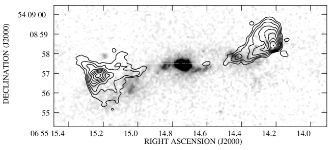
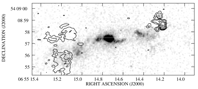
Figure 1: 8.1 GHz VLA image, made with VLA A-configuration data (see the text). Above is the total intensity image (contours at $300\times(1,2,4\dots)$ $\mu$Jy beam^-1; below is the polarized intensity image (contours at $150\times(1,2,4\dots)$ $\mu$Jy beam^-1. The restoring beam is an $0.29\times 0.20$-arcsec elliptical Gaussian in PA $-79$°. The greyscale shows a 3000-s exposure in the FR680 ramp filter of the HST’s WFPC2, kindly supplied by Clive Tadhunter, and is dominated by emission from the [OIII] 495.9/500.7 nm lines. Note the strong relationship between depolarization and emission-line regions.

2 Observations and analysis

The degree of depolarization is in general expected to be reduced at higher frequencies and higher resolutions. As parts of 3C 171’s hotspots had been found to be completely depolarized at the full resolution of the VLA ($\sim 0.25$ arcsec) at 8.1 GHz, I elected to observe the source with the A and B arrays of the VLA at the U and K bands, $\sim 15$ and $\sim 22$ GHz. In addition, I made use of the A-array 8.1-GHz observations discussed by Hardcastle et al. (1997).

Details of the observations used are listed in Table 1. The new observations were carried out in fast-switching mode with an integration time of 3.3 s, using frequent observations of a nearby bright point-source calibrator, 0749+540. The cycle time used was 320 s, with 80 s on calibrator and 240s on source, giving typical times of 50 s on the calibrator and 210 s on source after dead time due to slewing. (The low efficiency was due to the lack of a good nearby calibrator.) Primary referenced pointing was carried out, using short X-band observations of 0749+540 taken every hour, to avoid loss of sensitivity due to VLA pointing errors. The observations were made with two nearby observing frequencies (Table 1) with a 50-MHz bandwidth in each. 3C 286 was used as the flux and polarization position angle calibrator. The data were reduced in a standard manner within aips. elint was used to correct for the dependence of antenna gain on elevation. The use of fast-switching mode led to observations which were very well phase- and amplitude-calibrated after the standard calibration procedure: however, there was enough signal for a single iteration of phase self-calibration for each dataset, which gave a marginal improvement in image quality. Finally, the A- and B-array datasets were combined using dbcon, uvfix was used to align the datasets at the three wavelengths at the radio core, using the K-band dataset as the reference, and final images were made using imagr, combining the data from the two observing frequencies in each band. This resulted in images at effective frequencies of 8.09, 14.94 and 22.46 GHz. For simplicity, these frequencies will be referred to as 8, 15 and 22 GHz from now on.

Table 1: VLA observations

Array	Band	Observing frequencies		Date	Integration
		(GHz)			time (h)
A	X	8.065	8.115	1995 Aug 06	1
A	U	14.915	14.965	2001 Jan 16	4
A	K	22.435	22.485	2001 Jan 16	4
B	U	14.915	14.965	2001 Apr 01	1
B	K	22.435	22.485	2001 Apr 01	3

3 Results

Initially, images at the full resolution of the data were made: the image properties are listed in Table 2. These images were made using a matched shortest baseline of 18 k$\lambda$, and so are in principle sensitive to structures on the same angular scales: in practice, however, large-scale structure is resolved out at higher frequencies, and the steep spectrum of the source at high frequencies (Blundell 1996) also reduces the probability of detecting the lobes at 15 and 22 GHz.

Table 2: Resolutions and off-source noise levels of radio images

Frequency	Image	Noise ($\mu$Jy beam-1)
(GHz)		Stokes $I$	Stokes $Q$	Stokes $U$
8	$0.29\times 0.20$, $-79$°	54	33	33
15	$0.14\times 0.12$, $-87$°	49	47	46
	$0.30\times 0.20$, $-80$°	76	44	42
	(matched to 8-GHz)
22	$0.10\times 0.09$, $-81$°	37	33	33
	$0.14\times 0.12$, $-87$°	40	28	27
	(matched to 15-GHz)
	$0.30\times 0.20$, $-80$°	74	44	42
	(matched to 8-GHz)

In total intensity, the differences between the images are therefore predictable. The radio core is detected at all three frequencies, with flux densities of 1.8, 3.4 and 2.5 mJy at 8, 15 and 22 GHz respectively, giving it a steep spectrum at the higher frequencies. The only particularly notable feature to emerge from the new data is the compactness of the hotspots, which are only just resolved at the full resolution at 22 GHz, and are therefore only tens of milliarcsec (hundreds of pc) in size (Fig. 2). The W hotspot shows a well-resolved extension to the N, which may be tracing the current direction of outflow from the hotspot, while the E hotspot shows a striking bow-shock-shaped extension around the central compact component, superposed on a N-S filament. The hotspots have steep spectra at these high frequencies: the integrated spectral indices in the hotspots are $\alpha_{8}^{15}=0.92$ and $\alpha_{15}^{22}=1.38$ (W hotspot) and $\alpha_{8}^{15}=1.08$ and $\alpha_{15}^{22}=1.58$ (E hotspot).

Figure 2: The hotspots of 3C 171 at full resolution at 15 GHz (top, $0.14\times 0.12$ arcsec) and 22 GHz (bottom, $0.10\times 0.09$ arcsec). The off-source noise levels in the two images are given in Table 2. The lowest contour level is the $3\sigma$ level and the contours are logarithmic, increasing by a factor 2. Negative contours are dashed. Polarization vectors are perpendicular to the direction of the $E$-vector, and so would show magnetic field direction in the absence of Faraday rotation. Their lengths indicate relative fractional polarization. Polarization vectors are oversampled by a factor $\sim 2$ for visibility. Boxes on the lower panels show the regions used for integration of total and polarized intensity: see the text.

In polarization, however, the data clearly show the E hotspot to be polarized at 15 and 22 GHz, although it is essentially unpolarized at 8 GHz and below. The partial depolarization of the W hotspot also disappears at high frequencies. Some of this might be thought to be due to simple beam depolarization in the low-resolution 8-GHz images: there clearly is some polarization structure in the E hotspot in the images of Fig. 2. To investigate this, I made images at lower resolutions, matched to the resolution of the 8-GHz data, using appropriate weighting and tapering of the $u,v$ plane, and compared the integrated total and polarized fluxes of the two hotspots at different resolutions using the AIPS verb imstat, measuring using boxes which are shown in Fig. 2. Beam depolarization effects should be independent of frequency, to a first approximation, although the effects of spectral index mean that we are not seeing exactly the same structures at each frequency: considering the hotspot regions only should minimize these effects. Depolarization due to a Faraday-rotating medium should have a strong frequency dependence. The results of the measurements are given in Table 3.

It can be seen from these measurements that the dominant effect is frequency-dependent. The fractional polarization of the two hotspots increases with increasing frequency even in images made with matched resolutions. The total polarized flux remains approximately constant with frequency in the W hotspot and increases with frequency in the E hotspot. Since the flux measured in total intensity falls steeply with frequency, we can be certain that this is not simply a spectral index effect: a contaminating, highly-polarized component would have to have a flat or inverted spectral index. There is some evidence for beam depolarization effects in the differences between the fractional polarizations observed at different resolutions with the same frequency, particularly at 22 GHz, but this is clearly not the most significant effect.

There is some limited evidence for Faraday rotation associated with the region of depolarization. This is illustrated in Fig. 3, which shows the depolarization and rotation between 15 and 22 GHz at a resolution matched to the 8-GHz map. The most significant rotation is in the N part of the E hotspot. However, there is no particularly strong relationship between Faraday rotation and depolarization, and the rotation is never particularly large (modulo possible 180° rotation effects).

Table 3: Total and polarized flux measurements of the E and W hotspots

Hotspot	Freq.	Image	Total flux	Polarized	Fractional
	(GHz)		(mJy)	flux (mJy)	polarization
					(per cent)
W	8	Full	149.0	$6.5\pm 0.1$	$4.4\pm 0.1$
	15	8	84.5	$9.6\pm 0.1$	$11.4\pm 0.1$
	15	Full	86.1	$10.3\pm 0.2$	$12.0\pm 0.2$
	22	8	48.2	$6.7\pm 0.1$	$13.9\pm 0.2$
	22	15	49.4	$7.5\pm 0.1$	$15.1\pm 0.2$
	22	Full	49.2	$7.7\pm 0.2$	$15.7\pm 0.3$
E	8	Full	116.5	$0.6\pm 0.1$	$0.5\pm 0.1$
	15	8	60.1	$1.4\pm 0.1$	$2.3\pm 0.2$
	15	Full	60.9	$1.7\pm 0.2$	$2.7\pm 0.3$
	22	8	31.6	$1.8\pm 0.1$	$5.7\pm 0.3$
	22	15	32.6	$2.8\pm 0.1$	$8.2\pm 0.4$
	22	Full	32.3	$2.7\pm 0.2$	$8.6\pm 0.6$

The ‘Image’ column describes the resolution of the image used: ‘Full’ denotes the full resolution of the dataset, ‘8’ means matched to the 8-GHz dataset, and ‘15’ means that the image was matched to the 15-GHz dataset (the images are those described in Table 2). All images were made with matched shortest baselines. The errors on the polarized intensity are determined from the off-source r.m.s. noise in the Stokes $Q$ and $U$ images. Errors on the total intensity are similar in magnitude, but are not quoted as they are not a significant contributor to the errors in fractional polarization.

Figure 3: Depolarization and rotation between 15 and 22 GHz in the hotspots at $0.3\times 0.2$ arcsec resolution. The vector lengths show the ratio between the fractional polarizations at 15 and 22 GHz, with shorter vectors implying more depolarization. The longest vectors in both images correspond to a ratio of 1 (i.e., no depolarization). The vector direction shows the rotation between the two frequencies, with a vertical vector meaning no rotation, and positive rotations being counterclockwise. Only points with $3\sigma$ detections of total and polarized flux at both frequencies are plotted. Vectors are oversampled by a factor $\sim 2$.

4 Interpretation

We can begin by making the assumption that the depolarizing medium is external to the source. This is justified by the extremely good, though not perfect, association between the EELR and the depolarization. No model places the EELR inside the radio source – it is spatially quite distinct from, and physically larger than, the radio emission at various points (Fig. 1) – and at the same time it is clearly related to the depolarization. We can therefore treat the depolarizing material as an external screen of dimensions comparable to those of the EELR.

The situation is then a classical problem in the theory of radio polarization, discussed by Burn (1966). If a screen is external, two extreme cases can be identified. In the first, the Faraday screen is fully resolved by the telescope beam: in this case, no depolarization should be observed, but Faraday rotation should be seen. Some sources in rich cluster environments appear to be in this regime, in that the Faraday screen is partially or fully resolved (e.g. Perley & Carilli 1996). In 3C 171, however, we see significant depolarization without much associated Faraday rotation, as Fig. 3 shows. This is likely to be due to a largely unresolved foreground screen. In the limit that the size scale $d$ of the individual depolarizing regions (regions of uniform magnetic field) is much smaller than the resolution element, and is well defined, and that there are many regions along each line of sight, the degree of polarization $p$ of a part of the source seen through such a screen at a given frequency $\nu$ is given by

$$p=p_{i}\exp\left[-2K^{2}(n_{e}B_{\parallel})_{f}^{2}dRc^{4}\nu^{-4}\right]$$ (1)

(Burn 1966) where $p_{i}$ is the intrinsic polarization, $K$ is a constant with value $8.12\times 10^{-3}$ rad nT^-1 m kpc^-1, $(n_{e}B_{\parallel})_{f}^{2}$ is the dispersion in the product of number density and magnetic field strength and $R$ is the line-of-sight depth through the medium.

We can try to apply this model to the observations, but there are a number of reasons why it should be treated with caution. The first is a practical one: the measurements of the polarized intensity of the hotspots clearly include regions with different degrees of polarization (Fig. 3) and so, presumably, different physical conditions in the depolarizing screen. At best we will obtain some emission-weighted average of the physical conditions. To reduce this effect, I consider below only the E hotspot, which exhibits more uniform depolarization. The model is also not realistic. It assumes a single physical size scale for the variations in Faraday depth, parametrized by $d$. As Laing (1984) points out, realistic screens will have a range of scale sizes, which tends to wash out the sharp cutoff in polarization at low frequencies. This is probably the case for our observations: the degree of polarization at 8 GHz, though low, is still too high to be fitted with a simple model of the form of eq. 1. If we write eq. 1 as $p=p_{i}\exp(-C\nu^{-4})$, then we can solve for $C$ and $p_{i}$ using the 15 and 22 GHz data at $0.3\times 0.2$-arcsec resolution, obtaining (for the E hotspot) $C\sim 1.3\times 10^{41}$ Hz⁴, $p_{i}=7.1$ per cent: we would then expect the degree of polarization at 8 GHz to be essentially zero (about $10^{-5}$ per cent) whereas in fact there is a detection of polarization in this region at the $5\sigma$ level (Table 3). The intrinsic polarization $p_{i}$ obtained here is also somewhat low, which suggests that the model is not accurate even for the two higher frequencies. However, the value of $C$, which is the critical quantity for estimating physical parameters, simply depends logarithmically on the ratio of the polarizations at the two frequencies, and so is unlikely to be grossly wrong. Applying the model, we can see from the HST data, assuming a cylindrical symmetry, that $R\sim 5$ kpc: this would imply $(n_{e}B_{\parallel})_{f}d\approx 2\times 10^{5}$ m^-3 nT kpc^-1. If we further assume a simple model in which the differences are due to varying orientations of the magnetic field in an approximately uniform-density (though possibly low-filling-factor) medium, then, dropping numerical factors of order unity, $n_{e}Bd\approx 10^{5}$ m^-3 nT kpc^-1. (If there are in fact variations in $n_{e}$, then the $n_{e}$ value derived from this equation is a weighted average.)

Unfortunately, none of these three parameters, $n_{e}$, $B$ and $d$, is well constrained by existing observations. $B$ values of the order of 1 nT are energetically plausible from equipartition arguments, but this estimate is good to an order of magnitude at best. We know that $d<1$ kpc for the model above to be either necessary or applicable; the fact that the degree of polarization of the hotspots continues to increase at higher radio resolutions (Table 3) suggests, however, that at least some structure is present on scales $\sim 100$ pc.

The density is the most problematic quantity. Clark et al. (1998) suggested that the density in the emission-line clouds in the nuclear regions is $\sim 300$ cm^-3, but were unable to make measurements near the hotspots. Electron densities $\sim 100$ cm^-3 are often quoted for EELR. However, it is important to emphasise that it is probably not the line-emitting material itself that is depolarizing the radio source, if it has a density close to this value. Baum & Heckman (1989) estimate constraints on the density and mass of the extended line-emitting material in 3C 171, based on the observed H$\alpha$ luminosity and assuming case B recombination: for a filling factor of unity, they estimate $n_{e}=0.2$ cm^-3. To obtain a density $\sim 100$ cm^-3, a filling factor of $\sim 10^{-6}$ would be required: in other words, if the line-emitting material has this density, it will have a very low covering fraction, and cannot be responsible for depolarizing the radio source. For filling factors close to unity, a single-phase medium with a density close to the value given by Baum & Heckman can still just about explain the observations, requiring $d\sim 1$ kpc for $B=1$ nT. However, if the EELR consists of dense ($\sim 100$ cm^-3), warm line-emitting clouds with a low filling factor, they cannot be responsible for the observed depolarization. It must instead be due to a second phase of the ISM. A plausible candidate is a second, hotter, more diffuse ionized phase, which would be expected to be present in shock-ionization models for the EELR: if the two phases are in approximate pressure equilibrium, then the density of the hot phase can be much lower than in the EELR clouds. If we take $d\approx 100$ pc and $B\approx 1$ nT, then the depolarization implies $n_{e}\approx 1$ cm^-3, which is a plausible density for the hot phase in the above scenario. For pressure balance with the colder, denser EELR clouds, that density would imply $T_{\rm hot}\sim 10^{6}$ K: of course, we have no particular a priori reason to expect exact pressure balance in this dynamic situation.

The non-detection of 3C 171 in a deep ROSAT X-ray observation (Hardcastle & Worrall 1999) sets quite strict limits on the properties of any hot gas in the system. I derive a $3\sigma$ upper limit on the absorbed ROSAT-band (0.1–2.4-keV) flux of the region of interest of $\sim 3\times 10^{-14}$ ergs cm^-2 s^-1. If we again assume cylindrical symmetry, with $R=5$ kpc and $l\approx 50$ kpc, and consider a uniform medium, then Fig. 4 shows the constraints on gas density and temperature imposed by the X-ray limit together with the detection of depolarization. It can be seen that plasma of the temperature typically detected in the atmospheres of elliptical galaxies ($T\ga 10^{7}$ K) cannot be responsible for the depolarization: to avoid detection in the X-ray, its density would have to be low ($10^{-2}$ – $10^{-3}$ cm^-3), implying scales $d>1$ kpc, which would be resolved by the radio data. This conclusion is valid so long as $B$ is not very much larger than 1 nT. The allowed region of parameter space in Fig. 4 is more or less consistent, given the large uncertainties in all quantities involved (the calculation is particularly uncertain at low temperatures), with the order of magnitude estimate of the temperature of the ‘hot’ depolarizing medium given above: the X-ray data favour somewhat lower temperatures if $n_{e}\sim 1$ cm^-3, $T\la 3\times 10^{5}$ K. In the alternative scenario, involving a low-density EELR region, we expect $T_{\rm EELR}\approx 10^{4}$ K, which of course is entirely consistent with the X-ray upper limit.

Gas at temperatures around $10^{6}$ K can also in principle be detected in the optical via coronal emission lines (e.g. Graney & Sarazin 1990). If we adopt $n_{e}\approx 1$ cm^-3, then we can estimate upper limits on the temperature of the gas given the non-detection of any coronal lines in the spectra of Clark et al.. Graney & Sarazin’s results suggest that the most significant line for a plasma in ionization equilibrium (not necessarily a good model for the material we are considering!) with $T<10^{6}$ K is the [Fe X] 637.4 nm line. We derive an upper limit on the flux of this line from Clark et al.’s detection of [O I] at 636.3 nm, giving $F_{\rm[Fe\ X]}\la 4\times 10^{-16}$ ergs cm^-2 s^-1. For $n_{e}\approx 1$ cm^-3, given our adopted geometry and the size of the extraction region of Clark et al.  we require the emissivity coefficient $\Lambda_{\rm[Fe\ X]}\la 3\times 10^{-27}$ ergs cm³ s^-1. From Figure 1 of Graney & Sarazin, this corresponds to $T\la 6\times 10^{5}$ K; higher temperatures in the $10^{5.5}$–$10^{6.5}$ K region would have given rise to detectable [Fe X] emission in the optical spectra. Thus the optical data, like the X-ray data, favour temperatures somewhat lower than $10^{6}$ K for the hot phase. Again, this conclusion is sensitive to the choices of $d$ and $B$, which determine the adopted value of $n_{e}$. Values of $B$ larger than 1 nT allow lower $n_{e}$ values and a hotter plasma. In addition, it is sensitive to the metallicity and ionization mechanism of the hot phase, which are unknown; the key point here is simply to show that the presence of this phase is not ruled out by existing optical observations.

Figure 4: Constraints on the properties of the depolarizing medium. The solid line shows the upper limit on the electron density of the medium as a function of temperature given the ROSAT upper limit discussed in the text. Only regions of parameter space below and to the left of the solid line are permitted by the X-ray upper limit: higher densities or temperatures would produce more X-ray emission than observed. The calculation was carried out using the mekal model within xspec, assuming 0.5 solar abundances. The dashed line shows the constraint imposed by the fact that the depolarizing medium is not resolved ($d<1$ kpc), assuming $B=1$ nT. Only regions of parameter space above this line are permitted by the data, given equation 1. The exact position of the dashed line depends on the magnitude of $B$, and so is uncertain, as discussed in the text. The dotted line shows, for reference, the line of pressure balance with a gas of $T=10^{4}$ K, $n_{e}=100$ cm^-3 (plausible parameters for the EELR clouds).

To summarize, we are forced to one of two conclusions: either the EELR regions are very much less dense than the ‘typical’ numbers quoted for $10^{4}$-K emission-line gas, and are distributed not in clumps but in a uniform screen across the source; or, more probably, a second, less dense phase of the ISM, with $n_{e}\sim 1$ cm^-3 and a temperature likely to be around a few times $10^{5}$ K, is responsible for the depolarization. This second phase is plausibly shocked warm diffuse gas in the galaxy. In either case, the mass of the depolarizing medium, assuming it is cospatial with the EELR, would be $\sim 10^{10}$ M_☉.

References

- [] Baum, S.A., Heckman, T., 1989, ApJ, 336, 681
- [] Blundell, K.M., 1996, MNRAS, 283, 538
- [] Burn, B.J., 1966, MNRAS, 133, 67
- [] Clark, N.E., Axon, D.J., Tadhunter, C.N., Robinson, A., O’Brien, P., 1998, ApJ, 494, 546
- [] de Koff S., Baum, S.A., Sparks, W.B., Biretta, J., Golombek, D., Machetto, F., McCarthy, P., Miley, G.K., 1996, ApJS, 107, 621
- [] Graney, C.M., Sarazin, C.L., 1990, ApJ, 364, 561
- [] Hardcastle, M.J., Alexander, P., Pooley, G.G., Riley, J.M., 1997, MNRAS, 288, 859
- [] Hardcastle, M.J., Worrall, D.M., 1999, MNRAS, 309, 969
- [] Heckman, T.M., van Breugel, W.J.M., Miley, G.K., 1984, ApJ, 286, 509
- [] Laing, R.A., 1984, in Bridle A.H., Eilek J.A., eds, Physics of Energy Transport in Radio Galaxies, NRAO Workshop no. 9, NRAO, Green Bank, West Virginia, p. 90
- [] McCarthy, P.J., 1993, ARA&A, 31, 639
- [] McCarthy, P.J., Baum, S., Spinrad, H., 1996, ApJS, 106, 281
- [] McCarthy, P.J., van Breugel, W., Spinrad, H., Djorgovski, S., 1987, ApJ, 321, L29
- [] Perley, R.A., Carilli, C.L., 1996, in Carilli C.L., Harris D.E., eds, Cygnus A — Study of a Radio Galaxy, Cambridge University Press, Cambridge, p. 168
- [] Tadhunter, C.N., Morganti, R., Robinson, A., Dickson, R., Villar-Martin, M., Fosbury, R.A.E., 1998, MNRAS, 298, 1035