Matching torsion $\Lambda-$term with observations

Taking into account a torsion field gives rise to a negative pressure contribution in cosmological dynamics and then to an accelerated behaviour of Hubble fluid. The presence of torsion has the same effect of a $\Lambda$-term. We obtain a general exact solution which well fits data coming from high redshift supernovae and Sunyaev-Zeldovich/X-ray method for the determination of cosmological parameters. On the other hand, it is possible to obtain observational constraints on the amount of torsion density. A dust dominated Friedmann behaviour is recovered as soon as torsion effects are not relevant.

PACS number(s): 98.80.Cq, 98.80. Hw, 04.20.Jb, 04.50

1 Introduction

A generalization of Einstein General Relativity can be obtained by considering a torsion tensor different from zero in ${\bf U}_{4}$ space-time manifold where connection is not symmetric [1, 2]. Such an approach is very interesting today in relation to several extended theories of gravity as Superstrings, Supergravity and Kaluza-Klein theories. In particular, torsion allows to include spin matter fields in General Relativity and the Einstein-Cartan-Sciama-Kibble (ECKS) theory is one of most serious attempt in this direction. However, not all the forms of torsion are directly connected to a spin counterpart as it is widely discussed in [3].

Now if some forms of torsion allow to take into account spin in General Relativity, it seems reasonable that they could have had some role into dynamics of the early universe when the number density of particles per volume was huge. The presence of torsion gives naturally a repulsive contribution to the energy-momentum tensor [4]. In fact, it is possible to show that for densities of the order of $10^{47}g/cm^{3}$ for electrons and $10^{54}g/cm^{3}$ for protons and neutrons, torsion could give observable consequences if all the spins of the particles result aligned. These huge densities can be reached only in the early universe so that cosmology is the only viable approach to test torsion effects [4]. However no relevant tests confirming the presence of torsion have been found until now and it is still an open debate if the space-time is a Riemannian ${\bf V}_{4}$ manifold or not. Considering cosmology and, in particular primordial phase transitions and inflation [4, 5, 6], it seems very likely that, in some regions of early universe, the presence of local magnetic fields could have aligned the spins of particles. At very high densities, this effect could influence the evolution of primordial perturbations remaining as an imprint in today observed large scale structures.

¿From another point of view, the presence of torsion could give observable effects without taking into account clustered matter but resulting as a sort of cosmological constant. Recent observations seem to point out that the universe is accelerating. Type Ia Supernovae (SNe Ia) [7], data coming from clusters of galaxies [8] and CMBR investigations [9] give observational constraints from which we deduce that the universe is spatially flat, low density and dominated by some kind of non-clustered dark energy. Such an energy, which is supposed to have dynamics, should be the origin of the observed cosmic acceleration.

In terms of density parameter, we have $\Omega_{m}\simeq 0.3\,,\Omega_{\Lambda}\simeq 0.7\,,\Omega_{k}\simeq 0.0\,,$ where $\Omega_{m}$ includes non-relativistic baryonic and non-baryonic (dark) matter, $\Lambda$ is the dark energy (cosmological constant, quintessence,..), $k$ is the curvature parameter of Friedmann-Robertson-Walker (FRW) metric.

Standard matter fluid as source of Einstein–Friedmann cosmological equations gives rise to expanding decelerated dynamics. To fit observations, non-standard forms of matter-energy have to be taken into account: the net effect should be to implement a sort of a cosmological constant which naturally gives rise to a negative pressure capable of implementing an accelerated cosmic expansion. On the other hand, Quintessence [10, 11, 12] generalizes this approach taking into account all the mechanisms which give rise to negative pressure regimes for cosmic fluid. In particular, scalar fields.

The cosmological constant problem is one of the main issue of modern physics since its value should provide the gravity vacuum state [13], should be connected to the mechanism which led the early universe to the today observed large scale structures [14, 15], and should predict what will be the fate of the whole universe (no–hair conjecture) [16].

In any case, we need a time variation of cosmological constant to get successful inflationary models, to be in agreement with observations, and to obtain a de Sitter stage toward the future. In other words, this means that cosmological constant has to acquire a great value in early epoch, it has to undergo a phase transition with a graceful exit and has to result in a small remnant toward the future coinciding with the observational constraints (coincidence problem).

The today observed accelerated cosmological behaviour should be the result of this dynamical process where the present value of cosmological constant is not fixed exactly at zero.

In this context, a fundamental issue is to select the classes of gravitational theories and conditions which ”naturally” allow to recover an effective cosmological constant without considering special initial data. Theories with torsion could match up this point, as we will see below, also if the coincidence problem (that is the fine tuning between huge initial values of $\Lambda$ and very thin today observed constraints) remain essentially unsolved.

This paper is organized as follows. Sec.2 is devoted to an essential summary of gravity with torsion. In Sec.3, we show how introducing torsion in cosmological dynamics gives rise to a negative pressure extra-term acting as a cosmological constant and we found a general cosmological solution. In Sec.4, we match such a cosmological solution with data coming from SNe Ia surveys and Sunyaev-Zeldovich/X-ray method. Sec.5 is devoted to discussion and conclusions.

2 Gravity with torsion

In this section, we give general definitions of torsion and associated quantities. We shall use the notation in [1] and in [3]. It is a convention to call U₄ a $4$-dimensional space-time manifold endowed with metric and torsion. The manifolds with metric and without torsion are labeled as V₄.

Torsion tensor $S_{ab}^{\phantom{ab}c}$ can be defined, in a ${\bf U}_{4}$ space-time manifold, using the antisymmetric part of the affine connection coefficients $\Gamma_{ab}^{c}$, that is

$$S_{ab}^{\phantom{ab}c}=\frac{1}{2}\left(\Gamma_{ab}^{c}-\Gamma_{ba}^{c}\right)\equiv\Gamma_{[ab]}^{c}\,,$$ (1)

where $a,b,c=0,\dots 3$.

In Einstein General Relativity, it is postulated that $S_{ab}^{\phantom{ab}c}=0$.

Often in the calculations, torsion occurs in linear combinations as in the contortion tensor, defined as

$$K_{ab}^{\phantom{ab}c}=-S_{ab}^{\phantom{ab}c}-S^{c}_{\phantom{c}ab}+S^{\phantom{a}c}_{b\phantom{c}{a}}=-K^{\phantom{a}c}_{a\phantom{c}b}\,,$$ (2)

and in the modified torsion tensor

$$T_{ab}^{\phantom{ab}c}=S_{ab}^{\phantom{ab}c}+2\delta^{\phantom{[a}c}_{[a}S_{b]}$$ (3)

where $S_{a}\equiv S_{ab}^{\phantom{ab}b}$.

According to these definitions, it follows that the affine connection can be written as

$$\Gamma_{ab}^{c}=\left\{{}^{c}_{ab}\right\}-K_{ab}^{\phantom{ab}c}\,,$$ (4)

where $\left\{{}^{c}_{ab}\right\}$ are the usual Christoffel symbols of the symmetric connection.

The torsion contributions to the Riemann tensor can be explicitly given by

$$R_{abc}^{\phantom{abd}d}=R_{abc}^{\phantom{abd}d}(\{\})-\nabla_{a}K_{bc}^{\phantom{b]c}d}+\nabla_{b}K_{ac}^{\phantom{ac}d}+K_{ae}^{\phantom{ae}d}K_{bc}^{\phantom{bc}e}-K_{be}^{\phantom{be}d}K_{ac}^{\phantom{ac}e}$$ (5)

where $R_{abc}^{\phantom{abc}d}(\{\})$ is the standard Riemann tensor of General Relativity.

¿From Eq.(5), the expressions for the Ricci tensor and the curvature scalar are

$$R_{ab}=R_{ab}(\{\})-2\nabla_{a}S_{c}+\nabla_{b}K_{ac}^{\phantom{ac}b}+K_{ae}^{\phantom{ae}b}K_{bc}^{\phantom{bc}e}-2S_{e}K_{ac}^{\phantom{ac}e}$$ (6)

and

$$R=R(\{\})-4\nabla_{a}S^{a}+K_{ceb}K^{bce}-4S_{a}S^{a}.$$ (7)

The closest theory to General Relativity containing torsion is the Einstein-Cartan-Sciama-Kibble (ECSK) theory. It is described by

$$L=\sqrt{-g}\left(\frac{R}{2k}+{{\cal L}}_{m}\right),$$ (8)

which is the Lagrangian density of General Relativity depending on the metric tensor $g_{ab}$ and on the connection $\Gamma_{ab}^{c}$. $R$ is the curvature scalar (7) and ${{\cal L}}_{m}$ the Lagrangian density of matter fields.

By the variation of the matter Lagrangian density with respect to the metric we get

$$\mbox{{\bf t}}^{ab}=\frac{\delta{\cal L}_{m}}{\delta g_{ab}},$$ (9)

which is the symmetric stress–energy tensor while the variation with respect to the contortion tensor

$$\tau_{c}^{\phantom{c}ba}=\frac{\delta{\cal L}_{m}}{\delta K_{ab}^{\phantom{ab}c}},$$ (10)

is the source of torsion. In many instances, it can be identified with a spin density, but there are many cases in which the source of the torsion field is not spin [3].

By the full variation of (8) and introducing the canonical energy-momentum tensor

$${\bf\Sigma^{ab}}={\bf t^{ab}}+{}^{*}\tilde{\nabla}_{c}(\tau^{abc}-\tau^{bca}+\tau^{cab})\,,$$ (11)

where we used the abridged notation ${}^{*}\tilde{\nabla}_{c}:=\tilde{\nabla}_{c}+2S_{cd}^{\phantom{cd}d}$, the following field equations are derived [1]

$$G^{ab}=8\pi G{\bf\Sigma}^{ab}\,,$$ (12)

and

$$T_{ab}^{\phantom{ab}c}=8\pi G\tau_{ab}^{\phantom{ab}c}\,,$$ (13)

where $c=1$, and the symbol $\tilde{\nabla}$ indicates covariant derivative with torsion.

Eqs.(12) generalize the Einstein equations in a $U_{4}$.

Eqs.(13) are algebraic so that it is always possible to cast Eqs.(12) in pure Einstein ones, by substituting the torsion terms with their sources. The result is the definition of an effective energy–momentum tensor as the source of the Riemannian part of the Einstein tensor [1]. In doing so, one obtains

$$G^{ab}(\{\})=8\pi G\tilde{\mbox{{\bf t}}}^{ab},$$ (14)

where $G^{ab}(\{\})$ is the Riemannian part of the Einstein tensor. The effective energy–momentum tensor is then

$$\tilde{\mbox{{\bf t}}}^{ab} = \mbox{{\bf t}}^{ab}+8\pi G\left[-4\tau^{ac}_{\phantom{ac}[d}\tau^{bd}_{\phantom{bd}c]}-2\tau^{acd}\tau^{b}_{cd}+\tau^{cda}\tau_{cd}^{\phantom{cd}b}\right.$$ (15)

$$+ \left.\frac{1}{2}g^{ab}(4\tau^{\phantom{e}c}_{e\phantom{c}[d}\tau^{ed}_{\phantom{ed}c]}+\tau^{ecd}\tau_{ecd})\right].$$

The tensor ${\bf t}^{ab}$ can be of the form

$$\mbox{{\bf t}}^{ab}=(p+\rho)u^{a}u^{b}-pg^{ab},$$ (16)

if standard perfect–fluid matter is considered.

These considerations are extremely useful for the following, since torsion contributions can be treated as additional perfect-fluid terms.

3 Cosmology with a torsion $\Lambda$-term

The totally antisymmetric part of torsion can be expressed by a 4-vector

$$\sigma^{a}=\epsilon^{abcd}S_{bcd}\,.$$ (17)

If one imposes to it the symmetries of a background which is homogeneous and isotropic, it follows that, in comoving coordinates, only the component $\sigma^{0}$ survives as a function depending only on cosmic time (see [3, 17, 18]).

For a perfect fluid, the Einstein-Friedmann cosmological equations can be written as

$$\frac{\ddot{a}}{a}=-\frac{4\pi G}{3}(\tilde{\rho}+3\tilde{p})\,,$$ (18)

and

$$\left(\frac{\dot{a}}{a}\right)^{2}+\frac{k}{a^{2}}=\frac{8\pi G}{3}\tilde{\rho}\,,$$ (19)

where $a(t)$ is the cosmological scale factor and $k=0,\pm 1$ is the spatial curvature constant. Energy density and pressure can be assumed in the forms [3, 17, 18]

$$\tilde{\rho}=\rho+f^{2}\,,\qquad\tilde{p}=p-f^{2}\,,$$ (20)

where $f$ is a function related to $\sigma^{0}$, while $\rho$ and $p$ are the usual quantities of General Relativity. This choice can be pursued since we can define $S_{abc}=S_{[abc]}=f(t)$ where $f(t)$ is a generic function of time which we consider as the source of torsion. For a detailed discussion of this point see [3]

As above, we can define a stress-energy tensor of the form

$$\mbox{{\bf t}}^{(tot)}_{ab}=(\tilde{p}+\tilde{\rho})u_{a}u_{b}-\tilde{p}g_{ab}\,,$$ (21)

which, by Eqs. (20), can be splitted as

$$\mbox{{\bf t}}^{(tot)}_{ab}=\mbox{{\bf t}}^{(matter)}_{ab}+\mbox{{\bf t}}^{(torsion)}_{ab}\,.$$ (22)

Due to the contracted Bianchi identity, we have

$$\mbox{{\bf t}}^{(tot);b}_{ab}=0\;;$$ (23)

from which, we can assume that (cfr. [19])

$$\mbox{{\bf t}}^{(matter);b}_{ab}=0\,,\qquad\mbox{{\bf t}}^{(torsion);b}_{ab}=0\,.$$ (24)

In the FRW space-time, (23) becomes

$$\dot{\tilde{\rho}}+3H(\tilde{\rho}+\tilde{p})=0$$ (25)

which is

$$\dot{\rho}+3H(\rho+p)=-2f\dot{f}\,.$$ (26)

¿From Eqs.(24), both sides of (26) vanish independently so that

$$f(t)=f_{0}=\mbox{constant.}$$ (27)

In other worlds, a torsion field gives rise to a constant energy density. Taking into account standard matter whose equation of state is defined into the above Zeldovich range, we obtain

$$\tilde{\rho}=\rho_{0}\left[\frac{a_{0}}{a}\right]^{3(\gamma+1)}+f_{0}^{2}\,.$$ (28)

Inserting this result into the cosmological equations, we obtain, in any case, a monotonic expansion being $f_{0}^{2}>0$, $\dot{a}^{2}>0$. We obtain an accelerated behaviour if

$$\rho+3p<2f_{0}^{2}\,,$$ (29)

so that acceleration depends on the torsion density.

In a dust-dominated universe, we have

$$\tilde{\rho}=\rho_{0}\left(\frac{a_{0}}{a}\right)^{3}+f_{0}^{2}\,,\qquad\tilde{p}=-f_{0}^{2}\,,$$ (30)

and then the general solution is

$$a(t)={\left(\frac{a_{0}^{3}\rho_{0}}{2f_{0}}\right)^{1/3}\left[\cosh(f_{0}t)-1\right]}^{1/3}\,.$$ (31)

Obviously, if $f_{0}t\rightarrow 0$, we have $\displaystyle{\cosh(f_{0}t)\simeq(f_{0}t)^{2}}$ and then $a\sim t^{2/3}$, as it has to be.

This results tell us that a $\Lambda$-term can be obtained without considering additional scalar fields in the dynamics but only assuming that the space-time is ${\bf U}_{4}$ (a manifold with torsion) instead of ${\bf V}_{4}$ (the standard Riemann manifold of General Relativity). The advantage to pass from ${\bf V}_{4}$ to ${\bf U}_{4}$ is due to the fact that the spin of a particle turns out to be related to the torsion just as its mass is responsible for the curvature. From this point of view, such a generalization includes the spin fields of matter into the same geometrical scheme of General Relativity [1].

In what follows, we will compare the obtained solution with data coming from observations.

4 Matching torsion $\Lambda$-term with observations

4.1 The Supernovae SNe Ia method

It is well known that the use of astrophysical standard candles provides a fundamental mean of measuring the cosmological parameters. Type Ia supernovae (SNe Ia) are the best candidates for this aim since they can be accurately calibrated and can be detected at enough high red-shift. This fact allows to discriminate among cosmological models. To this aim, one can fit a given model to the observed magnitude - redshift relation, conveniently expressed as :

$$\mu(z)=5\log{\frac{c}{H_{0}}d_{L}(z)}+25$$ (32)

being $\mu$ the distance modulus and $d_{L}(z)$ the dimensionless luminosity distance. The distance in the model we are considering is completely equivalent to the one in a spatially flat universe with a non-zero cosmological constant. Thus $d_{L}(z)$ is simply given as :

$$d_{L}(z)=(1+z)\int_{0}^{z}{dz^{\prime}[\Omega_{M}(1+z^{\prime})^{3}+\Omega_{tor}]^{-1/2}}\ .$$ (33)

where $\Omega_{tor}=1-\Omega_{M}$ plays the same role as the usual $\Omega_{\Lambda}$.

The distance modulus, as said, can be obtained from observations of SNe Ia. The apparent magnitude $m$ is indeed measured, while the absolute magnitude $M$ may be deduced from template fitting or using the Multi - Color Lightcurve Shape (MLCS) method. The distance modulus is then simply $\mu=M-m$. Finally, the redshift $z$ of the supernova can be determined accurately from the host galaxy spectrum or (with a larger uncertainty) from the supernova spectrum.

Our model can be fully characterized by two parameters : the today Hubble constant $H_{0}$ and the matter density $\Omega_{M}$. We find their best fit values minimizing the $\chi^{2}$ defined as :

$$\chi^{2}(H_{0},\Omega_{M})=\sum_{i}{\frac{[\mu_{i}^{theor}(z_{i}|H_{0},\Omega_{M})-\mu_{i}^{obs}]^{2}}{\sigma_{\mu_{0},i}^{2}+\sigma_{mz,i}^{2}}}$$ (34)

where the sum is over the data points [21]. In Eq.(34), $\sigma_{\mu_{0}}$ is the estimated error of the distance modulus and $\sigma_{mz}$ is the dispersion in the distance modulus due to the uncertainty $\sigma_{z}$ on the SN redshift. We have :

$$\sigma_{mz}=\frac{5}{\ln 10}\left(\frac{1}{d_{L}}\frac{\partial d_{L}}{\partial z}\right)\sigma_{z}$$ (35)

where we assume $\sigma_{z}=200\ \rm{km\ s^{-1}}$ adding in quadrature $2500\ \rm{km\ s^{-1}}$ for those SNe whose redshift is determined from broad features [21]. Note that $\sigma_{mz}$ depends on the cosmological parameters so that we will employ an iterative procedure to find the best fit values.

The High - z team and the Supernova Cosmology Project have detected a quite large sample of high redshift ($z\simeq 0.18-0.83$) SNe Ia, while the Calan - Tololo survey has investigated the nearby sources. Using the data in Perlmutter et al. [7] and Riess et al. [20], we have compiled a combined sample of 85 SNe as described in detail in [21]. We exclude 6 lixely outliers SNe as discussed in [7], thus ending with a total of 79 SNe. The results of the fit are presented in Fig.1 where we show the 1,2 and 3 $\sigma$ confidence regions in the $(\Omega_{M},H_{0})$ plane.

Figure 1: 1, 2 and 3$\sigma$ confidence regions in the $(\Omega_{M},H_{0})$ plane. The central dot represents the best fit values : $\Omega_{M}=0.3,H_{0}=65.4\ {\rm km\ s^{-1}\ Mpc^{-1}}$.

The best fit values (with $1\sigma$ error) turn out to be :

$$\Omega_{M}=0.30\pm 0.08\ \ ,\ \ H_{0}=65.4\pm 1.2\ km\ s^{-1}\ Mpc^{-1}\ .$$

which allow to conclude that a torsion $\Lambda$-term could explain observation very well. On the other hand, we can estimate the torsion density contribution which result to be :

$$f_{0}^{2}=(5.6\pm 0.7)\times 10^{-30}\ g\ cm^{-3}\,,$$

which is a good value if compared to the cosmological critical density. It is worthwhile to note that, in the case of SNe, the error on $H_{0}$ does not take into account systematic uncertainties due to possible calibration errors. Due to this reason it is so small with respect to other results in literature.

4.2 The Sunyaev-Zeldovich/X-ray method

Besides the above results, we can discuss how the Hubble constant $H_{0}$ and the torsion density parameter $\Omega_{\it tor}$ can be constrained also by the angular diameter distance $D_{A}$ as measured using the Sunyaev-Zeldovich effect (SZE) and the thermal bremsstrahlung (X-ray brightness data) for galaxy clusters. Distances measurements using SZE and X-ray emission from the intracluster medium are based on the fact that these processes depend on different combinations of some parameter of the clusters (see [22] and references therein). The SZE is a result of the inverse Compton scattering of the CMB photons of hot electrons of the intracluster gas. The photon number is preserved, but photons gain energy and thus a decrement of the temperature is generated in the Rayleigh-Jeans part of the black-body spectrum while an increment rises up in the Wien region. We will limit our analysis to the so called thermal or static SZE, which is present in all the clusters, neglecting the ${\it kinematic}$ effect, which is present in those clusters with a nonzero peculiar velocity with respect to the Hubble flow along the line of sight. Typically the thermal SZE is an order of magnitude larger than the kinematic one. The shift of temperature is:

$$\frac{\Delta T}{T_{0}}=y\left[x\,\mbox{coth}\,\left(\frac{x}{2}\right)-4\right],$$ (36)

where ${\displaystyle x=\frac{h\nu}{k_{B}T}}$ is a dimensionless variable, $T$ is the radiation temperature, and $y$ is the so called Compton parameter, defined as the optical depth $\tau=\sigma_{T}\int n_{e}dl$ times the energy gain per scattering:

$$y=\int\frac{K_{B}T_{e}}{m_{e}c^{2}}n_{e}\sigma_{T}dl.$$ (37)

In the Eq. (37), $T_{e}$ is the temperature of the electrons in the intracluster gas, $m_{e}$ is the electron mass, $n_{e}$ is the numerical density of the electrons, and $\sigma_{T}$ is the cross section of Thompson electron scattering. We have used the condition $T_{e}\gg T$ ($T_{e}$ is the order of $10^{7}\,K$ and $T$, which is the CBR temperature is $\simeq 2.7K$). Considering the low frequency regime of the Rayleigh-Jeans approximation we obtain

$$\frac{\Delta T_{RJ}}{T_{0}}\simeq-2y$$ (38)

The next step to quantify the SZE decrement is the one to specify the models for the intracluster electron density and temperature distribution. The most commonly used model is the so called isothermal $\beta$ model [23]. We have

$$n_{e}(r)=n_{e}(r)=n_{e_{0}}\left(1+\left(\frac{r}{r_{e}}\right)^{2}\right)^{-\frac{3\beta}{2}}$$ (39)

$$T_{e}(r)=T_{e_{0}}~{},$$ (40)

being $n_{e_{0}}$ and $T_{e_{0}}$, respectively the central electron number density and temperature of the intracluster electron gas, $r_{e}$ and $\beta$ are fitting parameters connected with the model [24]. For the effect of the cluster modelling see [25]. From (6) we have

$$\frac{\Delta T}{T_{0}}=-\frac{2K_{B}\sigma_{T}T_{e_{0}}\,n_{e_{0}}}{m_{e}c^{2}}\cdot\Sigma$$ (41)

being

$$\Sigma=\int^{\infty}_{0}\left(1+\left(\frac{r}{r_{c}}\right)^{2}\right)^{-\frac{3\beta}{2}}dr\,.$$ (42)

The integral in Eq. (42) is overestimated since clusters have a finite radius. The effects of the finite extension of the cluters are analyzed in [25],[26].

A simple geometrical argument converts the integral in Eq. (42) in angular form, by introducing the angular diameter distance, so that

$$\Sigma=\theta_{c}\left(1+\left(\frac{\theta}{\theta_{2}}\right)^{2}\right)^{1/2-3\beta/2}\sqrt{\pi}\,\frac{\Gamma\left(\frac{3\beta}{2}-\frac{1}{2}\right)}{\Gamma\left(\frac{3\beta}{2}\right)}\,r_{DR}.$$ (43)

In terms of the dimensionless angular diameter distances, $d_{A}$ (such that $D_{A}=\displaystyle\frac{c}{H_{0}}d_{A}$) we get

$$\frac{\Delta T(\theta)}{T_{0}}=-\frac{2}{H_{0}}\frac{\sigma_{T}K_{B}T_{ec}n_{e_{0}}}{m_{e}c}\sqrt{\pi}\frac{\Gamma\left(\frac{3\beta}{2}\frac{1}{2}\right)}{\Gamma\left(\frac{3\beta}{2}\right)}\left(1-\left(\frac{\theta}{\theta_{2}}\right)^{2}\right)^{\frac{1}{2}(1-3\beta)}d_{A},$$ (44)

and, consequently, for the central temperature decrement, we get

$$\frac{\Delta T(\theta=0)}{T_{0}}=-\frac{2}{H_{0}}\frac{\sigma_{T}K_{B}T_{ec}n_{e_{0}}}{m_{e}c}\sqrt{\pi}\frac{\Gamma\left(\frac{3\beta}{2}\frac{1}{2}\right)}{\Gamma\left(\frac{3\beta}{2}\right)}\frac{c}{H_{0}}d_{A}.$$ (45)

The factor $\displaystyle\frac{c}{H_{0}}d_{A}$ in Eq. (45) carrys the dependence on the thermal SZE on both the cosmological models (through $H_{0}$ and the Dyer-Roeder distance $d_{A}$) and the redshift (through $d_{A}$). From Eq. (45), we also note that the central electron number density is proportional to the inverse of the angular diameter distance, when calculated through SZE measurements. This circumstance allows to determine the distance of cluster, and then the Hubble constant, by the measurements of its thermal SZE and its X-ray emission.

This possibility is based on the different power laws, according to which the decrement of the temperature in the SZE, $\frac{\Delta T(\theta=0)}{T_{0}}$ , and the X-ray emissivity, $S_{X}$, scale with respect to the electron density. In fact, as above pointed out, the electron density, when calculated from SZE data, scales as $d^{-1}_{A}$ ( $n^{SZE}_{e0}\propto d^{-1}_{A}$), while the same one scales as $d^{-2}_{A}$ ($n^{X-ray}_{e0}\propto d^{-2}_{A}$) when calculated from X-ray data. Actually, for the X-ray surface brightness, $S_{X}$, assuming for the temperature distribution of $T_{e}=T_{e0}$, we get the following formula:

$$S_{X}=\frac{\epsilon_{X}}{4\pi}{n_{e0}^{2}}\frac{1}{(1+z)^{3}}\theta_{c}\frac{c}{H_{0}}d_{A}I_{SX},$$ (46)

being

$$I_{Sx}=\int^{\infty}_{0}\left(\frac{n_{e}}{n_{e0}}\right)^{2}dl$$

the X-ray structure integral, and $\epsilon_{X}$ the spectral emissivity of the gas (which, for $T_{e}\geq 3{\times}10^{7}$, can be approximated by a typical value: $\epsilon_{X}=\epsilon\sqrt{T_{e}}$, , with $\epsilon\simeq 3.0{\times}10^{-27}n_{p}^{2}$ erg $cm^{-3}$ $s^{-1}$ $K^{-1}$ [24]) . The angular diameter distance can be deduced by eliminating the electron density from Eqs. (45) and (46), yielding:

$$\frac{y^{2}}{S_{X}}=\frac{4\pi(1+z)^{3}}{\epsilon}{\times}\left(\displaystyle\frac{k_{B}\sigma_{T}}{m_{e}c^{2}}\right)^{2}{T_{e0}}^{3/2}\theta_{c}\frac{c}{H_{0}}d_{A}{\times}\frac{\left[B(\frac{3}{2}\beta-\frac{1}{2},\frac{1}{2})\right]^{2}}{B(3\beta-\frac{1}{2},\frac{1}{2})}$$ (47)

where $B(a,b)=\displaystyle\frac{\Gamma(a)\Gamma(b)}{\Gamma(a+b)}$ is the Beta function.

It turns out that

$$D_{A}=\frac{c}{H_{0}}d_{A}\propto\frac{(\Delta T_{0})^{2}}{S_{X0}T^{2}_{e0}}\frac{1}{\theta_{c}},$$ (48)

where all these quantities are evaluated along the line of sight towards the center of the cluster (subscript 0), and $\theta_{c}$ is referred to a characteristic scale of the cluster along the line of sight. It is evident that the specific meaning of this scale depends on the density model adopted for clusters. In our calculations we are using the so called $\beta$ model.

Eqs. (47) allows to compute the Hubble constant $H_{0}$, once the redshift of the cluster is known and the other cosmological parameters are, in same way, constrained. Since the dimensionless Dyer-Roeder distance, $d_{A}$, depends on $\Omega_{{\it tor}}$, $\Omega_{m}$, comparing the estimated values with the theoretical formulas for $D_{A}$, it is possible to obtain information about $\Omega_{m}$ $\Omega_{{\it tor}}$, and $H_{0}$. Recently distances of 18 clusters with redshift ranging from $z\sim 0.14$ to $z\sim 0.78$ have been determined from a likelihood joint analysis of SZE and X-ray observation (see Table 7 [27] and reference therein). Modeling the intracluster gas as a spherical isothermal $\beta$-model allows to obtain constraints on the Hubble constant $H_{0}$ in a standard $\Lambda$-FRW model. We perform a similar analysis using angular diameter distances measurements for a sample of 44 clusters, constituted by the 18 above quoted clusters and other 24 already know data (see [22]). In Fig (2), our data are plotted against two theoretical models.

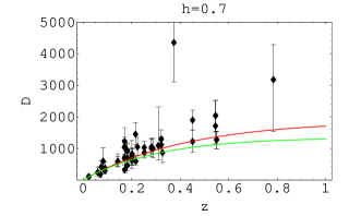
Figure 2: We plot the measure angular diameter distances with the error bars and two theoretical model: a Einstein- De Sitter model (bottom curve) and a flat $\Lambda$-FRW model with $\Omega_{m}=0.3$, $\Omega_{\Lambda}=0.7$ (upper curve), both with $H_{0}=70\ {\rm km\ s^{-1}\ Mpc^{-1}}$

As indicated in [22, 27], the errors $\sigma$ are only of statistical nature. Taking into account our model with torsion (31), the theoretical expression for the angular diameter distances $D_{A}$ is

$$D_{A}(z)=\frac{1}{(1+z)^{2}}d_{L}(z)=\frac{1}{1+z}\int_{0}^{z}{dz^{\prime}[\Omega_{M}(1+z^{\prime})^{3}+\Omega_{tor}]^{-1/2}}$$ (49)

We find the best fit values for $\Omega_{tor}$ and $H_{0}$, minimizing the reduced $\chi^{2}$:

$$\chi^{2}(H_{0},\Omega_{M})=\sum_{i}{\frac{[{D_{A}}^{theor}(z_{i}|H_{0},\Omega_{M})-{D_{A}}_{i}^{obs}]^{2}}{\sigma_{D_{A}}^{2}}}$$ (50)

The results are shown in the Fig. (3), where we see the contours corresponding to the $68.5\%$ and $98\%$ confidence levels:

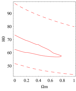
Figure 3: 1, $68.5\%$ and $98\%$ confidence regions in the $(\Omega_{M},H_{0})$ plane. The best fit values are : $\Omega_{M}=0.3,H_{0}=68\ {\rm km\ s^{-1}\ Mpc^{-1}}$.

The best fit values (at $1\sigma$) turn out to be :

$$\Omega_{M}=0.30\pm 0.3\ \ ,\ \ H_{0}=68\pm 6\ km\ s^{-1}\ Mpc^{-1}\ .$$

in good agreement with the above fit derived from SNe Ia data.

5 Discussion and conclusions

In this paper, we dealt with a cosmological model where torsion is present into dynamics. After the discussion of how such a contribution modifies cosmological Friedmann-Einstein equations, we have shown that the net effect of torsion is the introduction of an extra-term into fluid matter density and pressure which is capable of giving rise to an accelerated behaviour of the cosmic fluid. Being such a term a constant, we can consider it a sort of torsion $\Lambda$-term. If the standard fluid matter is dust, we can exactly solve dynamics which is in agreement with the usual Friedmann model (to be precise Einstein-de Sitter) as soon as torsion contribution approaches to zero.

The next step is to compare the result with observations in order to see if such a torsion cosmology gives rise to a coherent picture. We have used SNe Ia data, Sunyaev-Zeldovich effect and X-ray emission from galaxy clusters. Using our model, we are capable to reproduce the best fit values of $H_{0}$ and $\Omega_{M}$ which gives a cosmological model dominated by a cosmological $\Lambda$-term. In other words, it seems that introducing torsion (and then spins) in dynamics allows to explain in a natural way the presence of cosmological constant or a generic form of dark energy without the introduction of exotic scalar fields. Besides, as we have seen in Sec.4, observations allows to estimate torsion density which can be comparable to other forms of matter energy $(\sim 5.5\times 10^{-30}\,g\,cm^{-3})$.

However, we have to say that we used only a particular form of torsion and the argument can be more general if extended to all the forms of torsion [3]. Furthermore, being in our case the torsion contribution a constant density, it is not possible to solve coincidence and fine tuning problems. To address these issues we need a form of torsion evolving with time. This will be the topic of a forthcoming paper.

References

- [1] F.W. Hehl, P. von der Heyde, G.D. Kerlick and J.M. Nester, Rev. Mod. Phys. 48 (1976) 393.
- [2] A. Trautman Nature 242 (1973) 7.
- [3] S. Capozziello, G. Lambiase, and C. Stornaiolo Ann. Phys. (Leipzig) 10 (2001) 8, 713.
-
[4]
V. de Sabbata, Nuovo Cim. A 107 (1994) 363.
V. de Sabbata and C. Sivaram, Astr. and Space Sci. 165 (1990) 51;
V. de Sabbata and C. Sivaram, Astr. and Space Sci. 176 (1991) 141. -
[5]
E.W. Kolb, and M.S. Turner The Early Universe
Addison-Wesley 1990 (Redwood City, Calif.) -
[6]
P.J.E. Peebles Principle of Physical Cosmology,
Princeton Univ. Press 1993 (Princeton). -
[7]
B.P. Schmidt et al. Ap. J. 507, 46
(1998).
S. Perlmutter et al. Ap. J. 483, 565 (1997).
S. Perlmutter et al. Nature 391, 51 (1998).
S. Perlmutter et al. Ap. J. 517, 565 (1999). -
[8]
B. Chaboyer et al. Ap. J. 494, 96 (1998).
M.Salaris and A. Weiss Astron. Astrophys. 335, 943 (1998). - [9] P. de Bernardis et al. Nature 404, 955 (2000).
- [10] R.R. Caldwell, R. Dave, P.J. Steinhardt, Phys. Rev. Lett. 80, 1582 (1998).
-
[11]
R. de Ritis et al., Phys. Rev. D 62 (2000) 043506.
C. Rubano and J.D. Barrow, Phys. Rev. D64 (2001) 127301.
C. Rubano and P. Scudellaro, astro-ph/0103335 (2001). - [12] S. Capozziello, Int. Journ. Mod. Phys. D 11(2002) 483.
- [13] S. Weinberg, Rev. Mod. Phys. 61 (1989) 1.
- [14] A. Guth, Phys. Rev. D 23 (1981) 347; Phys. Lett. 108 B (1982) 389.
- [15] A.D. Linde, Phys. Lett. B 108, 389 (1982); Phys. Lett. B 114, 431 (1982); Phys. Lett. B 238 (1990) 160.
- [16] F. Hoyle and J.V. Narlikar, Proc. R. Soc. 273A (1963) 1.
- [17] H. Goenner and F. Müller-Hoissen, Class. Quantum Grav. 1 (1984) 651.
- [18] M. Tsamparlis Phys. Rev. D 24 (1981) 1451; Phys. Lett. A 75 (1979) 27.
- [19] P. Minkowski, Phys. Lett. B 173 (1986) 247.
- [20] A.G. Riess et al. Astron. J. 116 (1998) 1009 .
- [21] Y. Wang Ap. J. 536 (2000) 531.
- [22] M. Birkinshaw Phys. Rep. 310(1999) 97.
-
[23]
A. Cavaliere, R. Fusco–Femiano Astron. Astrophys. 49 (1976) 137.
A. Cavaliere, R. Fusco–Femiano Astron. Astrophys. 70 (1978) 677. - [24] C.L. Sarazin, “X-Ray Emission from Cluster of Galaxies”, Cambridge Univ. Press, Cambridge (1988).
- [25] D. Puy, L. Grenacher, Ph. Jetzer, M. Signore Astron. Astrophys. 362 (2000) 415.
- [26] Cooray A., 1998b, A&A, 333, L71.
- [27] Reese E. et al., astro-ph/0205350 (2002).