Determining Bolometric Corrections for BATSE Burst Observations

Abstract

We compare the energy and count fluxes obtained by integrating over the finite bandwidth of BATSE with a measure proportional to the bolometric energy flux, the $\varphi$-measure, introduced by Borgonovo & Ryde. We do this on a sample of 74 bright, long, and smooth pulses from 55 GRBs. The correction factors show a fairly constant behavior over the whole sample, when the signal-to-noise-ratio is high enough. We present the averaged spectral bolometric correction for the sample, which can be used to correct flux data.

1 Introduction

The gamma-ray burst (GRB) spectrum is often peaked in the $EF_{\rm E}$ representation (where $F_{E}$ is the energy flux) at some energy $E_{\rm pk}$ in the $\gamma$-ray band band93 . The limited spectral coverage of the used detector might affect the assigned measure of the total energy-integrated flux. To obtain a true bolometric flux a correction is needed. This is most important for the photon flux and less affects the energy flux as the energy spectrum is often peaked within the detector energy window.

To circumvent this issue Borgonovo & Ryde Borgonovo and Ryde (2001) proposed to use the value of $EF_{\rm E}$ at $E_{\rm pk}$ as a representation of the energy flux, since it is proportional to the bolometric flux. We denote this quantity by $\varphi$. It was shown that the power-law hardness-intensity correlations (HIC), that was studied for pulse decays, were better if the $\varphi$ value was used instead of integrating the energy flux over the BATSE band. This could indicate that the latter method suffers from effects which are not part of the correlation. The $\varphi$-method thus provides an efficient way of studying detailed features in the observed HICs.

This measure is limited to the cases where the peak actually exists within the studied band $[E_{\rm min},E_{\rm max}]$. Representing the spectrum by the Band et al. model band93 , this means that the low and high energy power law indices must have $\alpha>-2$ and $\beta<-2$. In the most common case where $E_{\rm max}>(\alpha-\beta)E_{\rm pk}/(\alpha+2)$, the proportionality between ${\varphi}$ and F=$\int F_{\rm E}dE$ becomes

$$\frac{F}{\varphi} \equiv k(\alpha,\beta,y_{\rm min},y_{\rm max})=\frac{e^{(\alpha+2)}}{(\alpha+2)^{\alpha+2}}$$ (1)

$$\times\left[\vphantom{\frac{(\alpha-\beta)^{\alpha-\beta}y_{\rm max}^{\beta+2}-(\alpha-\beta)^{\alpha+2}}{(\beta+2)e^{\alpha-\beta}}}\Gamma(\alpha+2)\{P(\alpha+2,\alpha-\beta)-P(\alpha+2,y_{\rm min})\}\right.$$

$$+\left.\frac{(\alpha-\beta)^{\alpha-\beta}y_{\rm max}^{\beta+2}-(\alpha-\beta)^{\alpha+2}}{(\beta+2)e^{\alpha-\beta}}\right],$$

where $y_{\rm min}=(\alpha+2)E_{\rm min}/E_{\rm pk}$, and $y_{\rm max}=(\alpha+2)E_{\rm max}/E_{\rm pk}$. $\Gamma(\alpha+2)$ and $P(\alpha+2,y)$ are the gamma function and the incomplete gamma function, respectively (see, e.g., Press et al. Press ). In the case that $\alpha$ and $\beta$ do not have a strong dependence on $E_{\rm pk}$, the only $E_{\rm pk}$ dependence in $k(\alpha,\beta,y_{\rm min},y_{\rm max})$ is in $y_{\rm min}$ and $y_{\rm max}$. In particular, when the integration is chosen over the whole energy range from $0$ to $\infty$, there will be no dependence at all. The $\varphi$-value can be interpreted as the integral over the whole energy range or, at least, over a range for which $y_{\rm min}<<1$ and $y_{\rm max}>>1$, and should, under some circumstances, be a better representation of the bolometric flux for the study of the hardness-intensity correlation.

Bolometric Correction to the Energy Flux

For this work, we use a sample of 74 pulses taken from 55 GRBs, observed by the Burst and Transient Source Experiment (BATSE) on the Compton Gamma-Ray Observatory. The burst data have a time resolution of multiples of 64 ms and the count flux is obtained by adding up the four energy channels from the Large Area Detectors (LADs) of BATSE. We search within bright bursts (with peak fluxes larger than 2 photons ${\rm s^{-1}cm^{-2}}$) for cases containing long, smooth pulse structures with a general “fast rise-slow decay”. The light curve for each burst in the sample was rebinned to achieve a signal-to-noise-ratio ($S/N$) of at least 30. All selected pulses have at least 4 time-bins at the given $S/N$. The spectrum for each time-bin was fitted with the Band et al. band93 model, allowing a deconvolution to find the energy spectrum and the peak energy. The energy spectrum was integrated over the energy band of the BATSE detector ($20-2000$ keV), for the strongest illuminated LAD, to find the instantaneous energy flux.

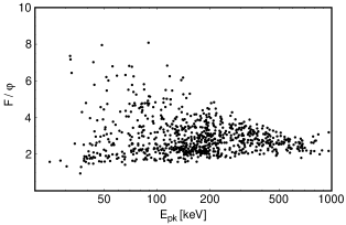
Figure 1: Ratio $F/\varphi$ versus $E_{\rm pk}$ for 846 time-resolved spectra from 55 GRBs. The integration of the energy flux $F$ was made over the range $20-2000$ keV.

In Figure 1, the spectral bolometric correction for 846 time-resolved spectra from the 55 GRBs is shown. Average values can be used to correct the energy flux data when $E_{\rm pk}=E_{\rm pk}(t)$ is known. The data show a greater dispersion for smaller $E_{\rm pk}$. This is most likely a bias introduced by the fact that most of the spectra correspond to the long decay phase of pulses, during which the intensity is positively correlated with the hardness. Therefore, the signal-to-noise ratio is usually much higher at the peak of the pulses when the spectra are harder, i.e., for higher $E_{\rm pk}$, and decreases to the chosen limit ($S/N=30$) as the pulse decays.

Bolometric Correction to the Count Observations

We now redo the above analysis on the count flux $F_{\rm c}$ instead. The count data have not been deconvolved and for proper physical interpretation the effective correction must be estimated and understood.

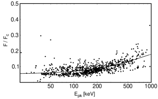
Figure 2: Ratio of the instantaneous energy flux to the count flux versus the corresponding $E_{\rm pk}$ (in keV), for the same sample of time-resolved spectra as in Fig. 1. A best-fit second-order polynomial $0.05235+1.924\times 10^{-4}E_{\rm pk}-6.624\times 10^{-8}E_{\rm pk}^{2}$ is also shown. The dispersion parameter is $0.1516$.

Figure 2 shows the ratio of the instantaneous energy flux $F$ (in keV ${\rm s^{-1}}{\rm cm^{-2}}$) to the corresponding count flux $F_{\rm c}$ (in counts ${\rm s^{-1}}$) for the same time-resolved spectra as in Figure 1. The data were fitted with a second-order polynomial which was found to be $0.05235+1.924\times 10^{-4}E_{\rm pk}-6.624\times 10^{-8}E_{\rm pk}^{2}$ (with $E_{\rm pk}$ given in keV). The dispersion was measured as the mean of the squared ratios between the fit residuals and the fit expected values. The $F/F_{\rm c}$ fit has a dispersion of 0.15.

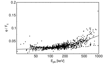
Figure 3: Ratio of the $\varphi$-measure to the count flux $F_{\rm c}$ versus $E_{\rm pk}$. A second-order polynomial fit to the data $0.01597+8.320\times 10^{-5}E_{\rm pk}-2.829\times 10^{-8}E_{\rm pk}^{2}$ is also shown. The dispersion parameter is $0.07605$.

In Figure 3, the ratio of the $\varphi$-measure (in keV ${\rm s^{-1}}{\rm cm^{-2}}$) to the count flux (in counts ${\rm s^{-1}}$) over the same sample of spectra is shown. Again the data were fitted with a second-order polynomial given by $0.01597+8.320\times 10^{-5}E_{\rm pk}-2.829\times 10^{-8}E_{\rm pk}^{2}$ (with $E_{\rm pk}$ in keV). This adjusts the data with higher accuracy for small $E_{\rm pk}$ values. The calculated dispersion is 0.08, significantly smaller than in the $F/F_{\rm c}$ case, shown in Figure 2.

Discussion

To interpret the BATSE spectral data, one must have in mind that due to the GRB spectra being broad compared to the observed energy window, one must apply a bolometric correction factor which is unknown. To circumvent this problem we propose the use of the $\varphi$ measure that is also proportional to the bolometric flux.

The flux $F$ is found from integrating the deconvolved spectrum. This spectrum is model-dependent as the deconvolution is based on the model spectrum. This could introduce additional scatter into the determination. A second problem, when one aims at studying single pulses in the light curve, arises from the fact that the observed spectra may contain contributions from other pulses which even could be unresolved. Furthermore, additional soft components Preece could also affect the measured flux value and thus weakening the correlations. This makes the $\varphi$-method better to use.

The $F/\varphi$ ratio shows an approximately constant behavior over the studied sample, with a larger dispersion for smaller $E_{\rm pk}$. This fact can be explained as a bias introduced by the HIC correlation.

We also analyze the correction for the count flux. The $\varphi/F_{\rm c}$ ratio is shown to have a substantially smaller dispersion than the $F/F_{\rm c}$ case. Therefore, the effective correction for the count flux may be better estimated.

References

- (1) Band, D., et al., ApJ 413, 281 (1993).
- Borgonovo and Ryde (2001) Borgonovo, L., and Ryde, F., ApJ 548, 770 (2001).
- (3) Press, W. H., Teukolsky, S. A., Vetterling, W. T., and Flannery, B. P., Numerical Recipes in Fortran 2nd Ed., Cambridge Univ. Press, Cambridge, 1992.
- (4) Preece, R. D., Briggs, M. S., Pendleton, G. N., et al., ApJ 473, 310 (1996).