Modelling the Recurrent Nova CI Aql in Quiescence

We present detailed photometric investigations of the recurrent nova CI Aql. New data obtained after the 2000 outburst are used to derive a 3D geometrical model of the system. The resulting light curves clearly indicate the existence of an asymmetric spray around the accretion disk, as claimed in the past e.g. for the super-soft X-ray source CAL87 in the LMC. The simulated light curves give us the mass transfer rates varying from $\dot{M}\approx 2.5\times 10^{-8}\,\,{\rm M}_{\odot}\,{\rm yr}^{-1}$ in 1991-1996 to $5.5\times 10^{-8}<\dot{M}<1.5\times 10^{-7}\,\,{\rm M}_{\odot}\,{\rm yr}^{-1}$ in 2001/2002. The distance and the interstellar foreground extinction resulting from the model are 1.55 kpc and E_B-V = 0$\aas@@fstack{m}$98 respectively. During fast photometry sequences in 2002 short timescale variations ($t_{\rm F}\approx 13$ minutes) of the mass loss are found. Moreover a change in the orbital period of the system is detectable and results in a mass loss of $2.2\times 10^{-6}<\Delta M<5.7\times 10^{-6}\,\,{\rm M}_{\odot}$ during the nova explosion.

1 Introduction

CI Aql is one of the 9 to 10 members of the class of recurrent novae: U Sco, V394 CrA, RS Oph, T CrB, V745 Sco, V3890 Sgr, T Pyx, CI Aql and IM Nor (Webbink et al. We87 (1987); Sekiguchi Sec (1995); Schmeja et al. schmeja (2000); Liller iauc7789 (2002)). Webbink et al. (We87 (1987)) also mention V1017 Sgr as possible class members although its status is still not clear. The first known outburst of CI Aql was discovered on Heidelberg plates recorded in June 1917 (Reinmuth ci_1 (1925)). Williams (ci_2 (2000)) completed the light curve by using records on Harvard College Observatory patrol plates. Schaefer (2001a ) found another outburst in 1941 again on Harvard plates. Schaefer argues, it might be a recurrent nova with a timescale of 20 years and the 1960 and 1980 outburst were missed. As the timescales of other recurrent novae often change and as there are no observations available, we assume for our calculations a quiescence phase of 60 years before the 2000 event. Anyway this does not affect the results of the model presented here but our resulting pre–outburst accretion rate indicates a long recurrence timescale. CI Aql was found to be an eclipsing binary system with a period of 0$\aas@@fstack{d}$618355(9) by Mennickent & Honeycutt (M_H (1995)). It is, to our knowledge, the only eclipsing system investigated photometrically in such detail before and after an outburst. Following the classification of Sekiguchi (Sec (1995)), CI  Aql is of U  Sco subclass (slightly evolved main sequence star and accreting white dwarf). For a detailed discussion of the outburst data we refer to Matsumoto et al. (Mat01 (2001)) and Kiss et al. (kiss (2001)).

In this paper we deduce a detailed model of the system basing on our optical photometry of 2001 and 2002. Further we follow the final decline to quiescence and find quasi periodic short timescale variations in this system. Together with pre–outburst data of Honeycutt (honey01 (2001)) we finally determine a period change.

2 The Data

The new data were obtained with the Innsbruck 60cm telescope (Kimeswenger ag01 (2001)) and a direct imaging CCD device in the period from June 21, 2001 to July 9, 2002. In 2001 a CompuScope Kodak 0400 CCD (4$\aas@@fstack{\prime}$6 $\times$ 3$\aas@@fstack{\prime}$1 field of view) was attached, in 2002 it was an AP7p SITe 502e (8$\aas@@fstack{\prime}$36 $\times$ 8$\aas@@fstack{\prime}$36). 781 images were taken in 34 nights with $V$, $R$ and $I_{\rm C}$ filters. The exposure times varied with filter, brightness, weather conditions and camera. Flatfield and bias subtraction were carried out in standard manner with the help of MIDAS routines. The source extraction was performed using SExtractor V2 (Bertin & Arnouts sex (1996)). The rms of the comparison standards in the field was $<0\aas@@fstack{m}08$ with the Kodak chip and $<0\aas@@fstack{m}05$ with the SITe CCD typically. The light curve was obtained by means of differential photometry of up to 40 stars within about 4$\aas@@fstack{\prime}$0 from the target in this very crowded field. For the absolute calibration CCD standards in the field by Henden & Honeycutt (H_H (1995)) and Henden (Henden01 (2001)) were applied. We found on that occasion that the coordinates of the whole set of the Henden & Honeycutt standards are shifted 1$\aas@@fstack{\prime}$73 east and 1$\aas@@fstack{\prime}$20 south and thus the finding chart overlay (SIMBAD/ALADIN) is wrong. As we use Johnson $R$ and the CCD standards of Henden (Henden01 (2001)) are taken in $R_{\rm C}$ we have to assume color terms in the absolute calibration. The attempt to derive these terms failed within the accuracy of the photometric data. We thus did not use the R band for the final results in extinction and distance (see section 5).

The pre–outburst data ranging from June 4, 1991 to September 29, 1996 were provided to us by Honeycutt (honey01 (2001)). The data consist of two sets (changing June 1995) with different zero points. The first set (the one used for Mennickent & Honeycutt M_H (1995)) was shifted according to the information given by Honeycutt to overlay. This corresponds well to the calibration of Skody & Howell (skody (1992)).

3 The Photometric Behavior

First of all we derived the ’remnant’ of the outburst in our 2001 data. The object clearly had not returned completely to quiescence as stated by Schaefer (2001b ) for August 4, 2001. To verify the real level, the new period (see section 7) was taken and the data points outside the primary eclipse were used to derive the final decline of the nova outburst. We see (Fig. 1) that this decline was finished somewhen in February/March 2002.

Figure 1: The final decline phase of the recent nova outburst (upper: $I_{\rm C}$; lower: $V$). Data around primary minima were removed to decrease effects due to the orbital modulation. First order polynomials to the 2001 data and second order polynomials to the whole data set are shown.

In contrast to this slowly continuous decline, the plateau phase in the model of Hachisu & Kato (HaKa (2001)) should stop abruptly when the super–soft X–ray source phase ends. The position for this end of the plateau phase depends strongly on the hydrogen content $X$. The overall evolution is shown in Fig. 2. We find that the decline started between JD 2452050 and JD 2452100.

Figure 2: The complete decline phase of the 2000 outburst (open symbols: CCD data from VSNET; closed symbols: our photometry). Due to the orbital modulation the upper boundaries have to be used. The ticks mark the predicted dates for the abrupt decline after the plateau for different hydrogen content $X$ (Hachisu & Kato HaKa (2001)).

Figure 3: The $V$ light curves for three different epochs: 1991-1996 (upper), 2001 (middle) and 2002 (lower panel). The light curve for 2001 was corrected according to the linear final decline shown above and normalized relative to October 1, 2001. The scatter is dominated by the short timescale variations (see section 6) and not by the errors in the data.

This results, including the late decline model calculations of Hachisu & Kato (HaKa (2001)), in a hydrogen content of $0.45<X<0.50$. This is in contradiction to Hachisu & Kato (HaKaII (2002)), who obtained a hydrogen poor model with $X=0.35$ on the basis of only two data points from the IAU Circulars of Schaefer (2001b , 2001c ). Our moderately hydrogen rich result is supported by the infrared spectroscopy of Lynch et al. (ci_6 (2002)) and by the first decline model (Fig. 4 in Hachisu & Kato HaKa (2001)).

The linear decline (Fig. 1) was subtracted to derive the light curve for 2001 which is shown together with those from the pre–outburst and from 2002 in Fig. 3. The periods and epochs used are described in section 7.

4 The 3D Model

The double star system was modelled with a slightly evolved main sequence secondary (SE) filling the Roche lobe, a nearly point source like, spherically symmetric white dwarf (WD), a rotationally symmetric inner accretion disk, a thin accretion stream from the Lagrange point towards the disk and a spray of bounced material first introduced by Schandl et al. (spray (1997)).

The WD mass of 1.2  M_⊙ was derived by Hachisu & Kato (HaKa (2001), Fig. 4) by means of the thick wind model of the early decline of the 1917 and the 2000 outburst. The mass of the SE can not be determined that directly. For a range of SE masses we used the evolutionary tracks and colors for solar abundance stars of Girardi et al. (tracks (2000)) and our 2002 photometry at minimum, when the SE dominates the emission. The point in the evolutionary track was chosen to fill the Roche lobe. This results in the extinction free ($V-I_{\rm C}$)₀ color. Together with our measured ($V-I_{\rm C}$) in 2002 and each SE mass we are able to derive a corresponding range for E_B-V. The results are summarized in Tab. 1.

Table 1: Extinction derived from ($V-I_{\rm C}$)${}_{minimum}=1\aas@@fstack{m}5$
and the evolutionary tracks at Roche lobe filling position.

$M_{\rm SE}$ $[$M${}_{\odot}]$	$R^{\rm RL}_{\rm SE}$ $[$R${}_{\odot}]$	$T_{\rm eff}$ $[$K$]$	($V-I_{\rm C}$)0	EB-V
1.4	1.65	6 690	0$\aas@@fstack{m}$488	0$\aas@@fstack{m}$82
1.5	1.69	7 040	0$\aas@@fstack{m}$405	0$\aas@@fstack{m}$90
1.6	1.74	7 380	0$\aas@@fstack{m}$307	0$\aas@@fstack{m}$97
1.7	1.78	7 760	0$\aas@@fstack{m}$214	1$\aas@@fstack{m}$04
1.8	1.83	8 110	0$\aas@@fstack{m}$132	1$\aas@@fstack{m}$10

According to van den Heuvel et al. (vH (1992)) a 1.4 M_⊙ ZAMS star as SE can already achieve a mass transfer, which leads to a steady hydrogen shell burning on the WD. A recurrent nova is not likely anymore below this mass limit. Thus a smaller SE does not have to be taken into account. On the other hand the $VI_{\rm C}JK_{\rm s}$ photometry of Schmeja et al. (schmeja (2000)) shortly after the outburst limits the interstellar extinction. The ($V-K_{\rm s}$)₀ as well as the ($I_{\rm C}-J$)₀ were calculated for different interstellar extinctions. They get to a negative domain at E${}_{\rm B-V}>1\aas@@fstack{m}05$. This is thus an upper limit for the extinction, assuming a dominant photosphere. Thus we conclude $1.4<{M}_{\rm SE}\leq 1.7$ M_⊙.

The geometric model was realized with the help of the ”MATLAB language of technical computing 5.3R11” (matlab (1999)). This allowed us to easily implement and modify various asymmetric surfaces, system inclinations and rotation periods. All surfaces are assumed to radiate like black bodies. The ray tracing for the irradiation within the system was solved explicitly. The ray tracings during system rotation for the resulting light curves were obtained by the internal renderer.

Figure 4: The basic geometric model with the Roche lobe filling SE, the symmetric accretion disk, the accretion stream and the spray of bounced material at the light curve phase of 0.33. The grid mesh density of the surfaces was reduced here for clarity by a factor of three with respect to the one used in the real calculations.

The model consists of the five components described in detail later. The resulting scheme is shown in Fig. 4. Each surface element was characterized by its temperature. To obtain the flux in each band, the contribution of each element was calculated by folding the black body with the filter curves ($B$, $V$, $R_{\rm C}$ and $I_{\rm C}$: Bessel bessel (1990); Johnson $R$: Aller et al. LB (1982)). For the zero point a spherical body simulating the sun was used in the same way in the renderer and calibrated by the values of Bessel et al. (bessel2 (1998)).

The White Dwarf

We assume a spherical WD photosphere. The luminosity of the WD is given by

$$L_{\scriptscriptstyle\rm WD}=L_{{\scriptscriptstyle\rm HSB}}+{1\over 2}\,{{\rm G}\,M_{\scriptscriptstyle\rm WD}\,\dot{M}\over R_{\scriptscriptstyle\rm WD}}$$ (1)

where $L_{{\scriptscriptstyle\rm HSB}}$ is the luminosity obtained from the remnant of the hydrogen shell burning in 2001 (Hachisu & Kato HaKa (2001)) and the second term originates from the accretion (Shaviv & Starrfield star87 (1987)). According to the model of Hachisu & Kato and the photometric behavior shown before, there is a remnant of the thermonuclear processes after the outburst in the 2001 data. The simulations give us $L_{{\scriptscriptstyle\rm HSB}}\approx 200\,$L_⊙. This results in a net hydrogen mass burning $\dot{M}_{\rm He}\approx 10^{-9}$  M_⊙ during the plateau phase from end 2000 to August 2001. This is just below ${}^{1}/_{10}$ of the mass-increase rate given by Hachisu & Kato for the total outburst.

The direct light contribution of the WD is negligibly small in our visual bands. It only contributes by the irradiation on the other components.

The Secondary

The shape of the secondary is calculated numerically. It starts in the inner critical Lagrange point which is fixed by

$$\left({2\pi\over P}\right)^{2}\left({\stackrel{{\scriptstyle\rightarrow}}{{r}}_{\!\scriptscriptstyle\rm CG,0}\cdot\stackrel{{\scriptstyle\rightarrow}}{{e}}_{\!\scriptscriptstyle 1}}\right)\,={{\rm G}M_{\scriptscriptstyle\rm WD}\over|{\stackrel{{\scriptstyle\rightarrow}}{{r}}_{\!\scriptscriptstyle\rm WD,0}}|^{2}}-\frac{{\rm G}M_{\scriptscriptstyle\rm SE}}{|{\stackrel{{\scriptstyle\rightarrow}}{{r}}_{\!\scriptscriptstyle\rm SE,0}}|^{2}}$$ (2)

where G is the gravitational constant and ${\stackrel{{\scriptstyle\rightarrow}}{{r}}_{\!\scriptscriptstyle\rm WD}}$, ${\stackrel{{\scriptstyle\rightarrow}}{{r}}_{\!\scriptscriptstyle\rm SE}}$ and ${\stackrel{{\scriptstyle\rightarrow}}{{r}}_{\!\scriptscriptstyle\rm CG}}$ the vectors to the WD, the SE and the center of gravity (CG) respectively. $\stackrel{{\scriptstyle\rightarrow}}{{e}}_{\!\scriptscriptstyle 1}$ is the unity vector parallel to ${\stackrel{{\scriptstyle\rightarrow}}{{r}}_{\!\scriptscriptstyle\rm CG}}-{\stackrel{{\scriptstyle\rightarrow}}{{r}}_{\!\scriptscriptstyle\rm SE}}$. An index 0 stands for values at the Lagrange point. The surface of the SE then follows the equipotential $\phi=\phi_{0}$ including the rotation of the complete binary flattening the system

$$\phi_{0}=-{\rm G}\,\,\left({{M_{\scriptscriptstyle\rm WD}\over|{\stackrel{{\scriptstyle\rightarrow}}{{r}}_{{\!\scriptscriptstyle\rm WD}}}|}+\frac{M_{\scriptscriptstyle\rm SE}}{|{\stackrel{{\scriptstyle\rightarrow}}{{r}}_{{\!\scriptscriptstyle\rm SE}}}|}}\right)-\frac{\pi}{P}\,\,\left({\stackrel{{\scriptstyle\rightarrow}}{{r}}_{\!\scriptscriptstyle\rm CG}\cdot\stackrel{{\scriptstyle\rightarrow}}{{e}}_{\!\scriptscriptstyle 1}}\right)^{2}$$ (3)

The calculated volume corresponds within one percent to the Roche lobe volume of Eggleton (roche (1983)).
The star is irradiated by the WD. This increases the undisturbed temperature $T_{*,0}$:

$$\sigma T_{*,irr}^{4}=\sigma T_{*,0}^{4}+\eta_{*}\,{L_{\scriptscriptstyle\rm WD}\over 4\pi r^{2}}\,\cos\theta$$ (4)

where $r$ is the distance of the surface element from the WD and $\theta$ the angle of incidence. An efficiency $\eta_{*}=0.7$ was used. The value results from fitting details of the light curve - mainly the gradient at phases 0.08 to 0.18. This somewhat higher value than that assumed in previous investigations may originate from the compact MS nature of the SE preventing the star from using the irradiated energy to change its internal structure. For the model this energy is distributed along the stellar surface (Fig. 5) in the same way as described in Schandl et al. (spray (1997)).

Figure 5: The effects of the redistribution of the temperature along the meridian from the inner critical Lagrange point (0°) to a pole (90°) and further to the backside of the SE (180°): thick line - redistributed temperature profile; thin line - original irradiated temperature $T_{*,irr}$.

The Disk

A rotational symmetric accretion disk was used. Elongated disks as they are proposed by Paczyński (rd_1 (1977)) or result from projecting the 3D disk models of Hirose et al. (3ddisk (1991)) were tested too but showed negligible effects. The horizontal size $R_{\rm D}=0.75R^{\scriptscriptstyle\rm RL}_{\scriptscriptstyle\rm WD}$ of the disk is determined by the stability due to tidal forces near the Roche lobe (Paczyńsky rd_1 (1977), Papaloizou & Pringle rd_2 (1977)). The width of the primary minimum independently leads us to the same result. The vertical height in the inner part ($r<R_{1}$) was obtained from the fit to the hydrodynamic models (Meyer & Meyer-Hofmeister MeMe (1982)) by Schandl et al. (spray (1997)). The calculations of Meyer & Meyer-Hofmeister (MeMe (1982)) show a rapid turnover of the vertical behavior. The lower gradient causes for those regions no irradiation by the WD anymore. Therefore we used

$$z=\left\{\begin{array}[]{l@{\quad}l}2.527\,\,r^{1.093}\,\,M_{\scriptscriptstyle\rm WD}^{-0.38}\,{\dot{M}}^{0.17}&:\quad r\leq R_{1}\\ &\\ const.&:\quad R_{1}\leq r\leq R_{\rm D}\end{array}\right.$$ (5)

where $z$, $r$, $R_{1}$, $M_{\scriptscriptstyle\rm WD}$ and ${\dot{M}}$ are in solar units. $R_{1}$ was estimated from Fig. 1 in Meyer & Meyer-Hofmeister (MeMe (1982)) for $M_{\scriptscriptstyle\rm WD}=1.2$ M_⊙ to be

$$R_{1}=0.365\,\log(\dot{M})+2.69$$ (6)

This description of the disk differs significantly from the parabolic law used by Hachisu & Kato (HaKa (2001)). They argue, referring to Schandl et al. (spray (1997)), that they simulate the ”flare–up” of the rim. But they increase strongly the reradiation of the WD flux on every part of the disk. This effect gets drastically at the outer disk portions. Moreover the high ”flare–up” built by the spray, as shown below, does not cover the whole rim but only about a quarter of it. Meyer & Meyer-Hofmeister (MeMe (1982)) also tested the effects of the irradiation on the vertical structure and found only marginal effects for CVs.
The disk temperature was adopted from the frictional heating and the surface irradiation as in Schandl et al. (spray (1997)) by

$$\sigma T_{\scriptscriptstyle\rm D}^{4}={3\over 8\pi}\,\,{{\rm G}M_{\scriptscriptstyle\rm WD}\,\dot{M}\over r^{3}}+\eta_{\scriptscriptstyle\rm D}\,{L_{\scriptscriptstyle\rm WD}\over 4\pi r^{2}}\,\cos\theta$$ (7)

For $T_{\scriptscriptstyle\rm D}<T_{\scriptscriptstyle ST}$ the stream temperature $T_{\scriptscriptstyle ST}$ (see description of the accretion stream later in this section) of the infalling material was assumed at the disk too. The efficiency parameter for the irradiation was assumed to be $\eta_{D}=0.5$, like in Schandl et al. (spray (1997)) and Hachisu & Kato (HaKa (2001)). Our tests with the models show nearly no noticeable effects on the composite light curve for slightly different $\eta_{D}$. The black body approximation fits very well for the disk in the visible spectral range as shown by recent full radiative transfer models (AcDc) producing artificial spectra (Nagel et al. AcDc (2002)).

The Spray

The spray was first introduced by Schandl et al. (spray (1997)) as convolute of individual blobs bounced after reaching the incident point of the accretion stream. Schandl et al. (spray (1997)) and Meyer-Hofmeister et al. (sprays (1997), short_time (1998)) found that the vertical extension dominates the effect on the light curve for the high inclination system here. Although they were able to calculate individual trajectories of undisturbed blobs the final, optically thick surface was modelled from the effects in the light curve (see Fig. 6).

Figure 6: The model for the different phases. The grey scale represents the $V$ flux intensity due to the temperature distribution.

Figure 7: The structure of the spray as top view (upper panel, including the circular disk) and its vertical structure projection (lower panel). The shape is symmetric with respect to the equatorial plane. The coordinates originate in the center of gravity (GC). For the stream the real trajectory is shown here. For the calculation a straight approximation was used.

We obtained the shape of the spray in the same way for our target (Fig. 7). The massiveness of the spray varied with the mass transfer rates.

The temperature of the irradiated regions of the spray were deduced according to Eqn. 4 with the stream temperature $T_{\scriptscriptstyle ST}$ as undisturbed value. Since the material consists of a clumpy medium the overall efficiency for heating due to irradiation is not comparable to a stellar photosphere. At short wavelength it is assumed that the spray is even half transparent (Meyer meyer_private (2002)) causing the observed super soft X-ray effects. We therefore found in the simulations the plausible value of $\eta_{S}=0.2$.

The Accretion Stream

The end points of the accretion stream are defined on the one hand by the Lagrange point and on the other hand by the impact point. The latter is calculated from an undisturbed gravitational particle trajectory towards the disk and characterized by the angle $\phi_{\scriptscriptstyle\rm S}$. As the bend of the trajectory is small (Fig. 7), a straight line was assumed. The cross–section of the stream is determined like in Meyer & Meyer-Hofmeister (MeMe83 (1983)) but slightly flattened. Recent hydrodynamic numerical simulations by Oka et al. (oka (2002)) show very similar deflection angles and tube geometries at $\tau\approx 1$.

The temperature $T_{\scriptscriptstyle ST}$ of the material is defined by the irradiated and distributed temperature of the SE at the stream source. The contribution of the stream to the light curve is rather small.

Figure 8:  The features used to limit independently different geometrical structures of the model (upper left panel). The data points for the individual epochs and colors together with the simulated curves are shown in the other panels. The crosses in the 2002 data from phase 0.55 to 0.68 correspond to data of two individual nights only. They seem do deviate systematically from the model. As shown later individual nights may vary due to variations in the accretion rate. We assume this sub–sample to be affected in such a way.

The Composition of the Modell

The individual components are dominating different parts of the light curve:

• The width of the central part of the primary minimum gives the disk size and limits the system inclination $i$.

• The depth of the primary and the secondary minimum strongly depend on the system inclination. Neither an inclination of 70° nor of 72° result in a usable fit, as in the first case the modelled primary minima are not deep enough for reasonable $\dot{M}$ and adjusted secondary minima, otherwise those of 2002 are too deep.

• The difference of the plateau levels before and after the secondary minimum gives the parameters of the secondary - namely the reduced irradiation by the shadow of the spray - and the irradiation efficiency of the spray.

• The depression of the late light curve gives length and height of the spray.

• The gradient of the late part of the primary minimum (phase: 0.08 - 0.18) gives the irradiation parameter $\eta_{\scriptscriptstyle\rm SE}$ of the SE

Figure 9: The contribution of the individual components to the total light curve in 2001 for $V$ (left) and $I_{\rm C}$ (right). The asymmetry of the spray causes a shift of the position in the primary eclipse. This is of special interest if combining data from different epochs (respectively mass transfer rates) for determination of the period.

X

Table 2: The parameters of the best fit model.

system:	i = 71$\degr$
secondary:	$M_{\scriptscriptstyle\rm SE}$ = 1.5 M⊙	$T_{\scriptscriptstyle\rm SE}$ = 7 000 K
white dwarf:	$M_{\scriptscriptstyle\rm WD}$ = 1.2 M⊙	$R_{\scriptscriptstyle\rm WD}$ = 0.0072 R⊙
disk:	$R_{\scriptscriptstyle\rm D}=0.75\,R^{\rm RL}_{\scriptscriptstyle\rm WD}$
stream:	$\phi_{\scriptscriptstyle\rm S}=$14$\aas@@fstack{\circ}$2
1991-1996	$\dot{\rm M}=2.5\times 10^{-8}\,\,$M⊙	$R_{1}=0.54\,R^{\rm RL}_{\scriptscriptstyle\rm WD}$
2001	$\dot{\rm M}=1.5\times 10^{-7}$	$R_{1}=0.75$
2002	$\dot{\rm M}=5.5\times 10^{-8}$	$R_{1}=0.72$

The parameters $M_{SE}$, $T_{SE}$, $i$, $\dot{M}$, $R_{D}$, $\eta_{*}$, $\eta_{D}$, $\eta_{S}$ and the spray geometry were varied independently in the beginning. The use of different photometric bands – namely $V$, $R$ and $I_{\rm C}$ – gives us further restrictions to the overlapping part of the possible individual solutions. Finally $M_{SE}$, $T_{SE}$, $i$, $\eta_{*}$, $\eta_{D}$ and $\eta_{S}$ are limiting the variation ranges between the years. The pre–outburst parameters are missing other bands than $V$ and thus are somewhat more flexible. The resulting simulated light curves are shown together with the data in Fig. 8. In Fig. 9 the individual contributions of the components to the total light curve are plotted.

5 Distance and Interstellar Extinction

The model light curves were derived independently for each band. When shifting those curves to the data we obtain for each band an optimized solution as function of the distance $D$ and the foreground extinction. Having more than two bands allows us to derive E_B-V (Fig. 10), using a standard model for the interstellar extinction (Mathis et al. MRN (1977)).

Kiss et al. (kiss (2001)) derive values of 0$\aas@@fstack{m}$83$\pm$0$\aas@@fstack{m}$20, 1$\aas@@fstack{m}$08$\pm$0$\aas@@fstack{m}$20 and 0$\aas@@fstack{m}$66$\pm$0$\aas@@fstack{m}$30 for the diffuse interstellar bands (DIB) at 584.9 nm, 661.3 nm and CaII 393.4 nm respectively. Using the photometries of Hanzl (hanzl (2000)) and Jesacher et al. (jesacher (2000)) on days +2 and +6 after maximum and the general tendency for novae around maximum of (B-V)₀ = 0$\aas@@fstack{m}$23$\pm 0$$\aas@@fstack{m}$06 (Kiss et al. kiss (2001)) we get $0\aas@@fstack{m}35<$E${}_{\rm B-V}<0\aas@@fstack{m}75$. But, as Kiss et al. point out already, those colors may be affected strongly by emission features. Hachisu & Kato (HaKa (2001)) derive from their model of the pre–outburst light curve E_B-V = 0$\aas@@fstack{m}$86. In their revision (Hachisu & Kato HaKaII (2002)), based on the early final $B$ band decline points of Schaefer (2001b , 2001c ) and thus the low hydrogen content (see section 3), they move it to E_B-V = 1$\aas@@fstack{m}$00. While the direct spectroscopic methods give similar results, the photometry suffers from the fact, that an average color for novae is assumed. The comparison with the models using the $B$ band may also suffer from the fact, that this band is mostly affected by the non grey opacities. A black body, as used by the models, may not work properly. We mostly rely on the direct spectroscopic methods and the models here using the red bands and thus use E${}_{\rm B-V}=0\aas@@fstack{m}98\pm 0\aas@@fstack{m}1$.

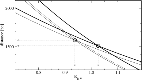
Figure 10: The distance as function of the interstellar extinction for different bands individually. The solutions are derived by the intersection of the pairs of each year. The thick lines are the solution for 2001 resulting in E${}_{\rm B-V}=1\aas@@fstack{m}025$. The thin lines represent the 2002 data giving E${}_{\rm B-V}=0\aas@@fstack{m}935$. The dashed line represents the pre–outburst data. Due to the lacking second photometric band, no solution is possible there. Nevertheless the tendency gives us some information on the accuracy of the solutions above.

The total luminosity also results from the simulations. This gives us a distance of 1.52 kpc to 1.58 kpc. Hachisu & Kato (HaKa (2001)) get 1.6 kpc from the maximum outburst brightness and using E${}_{\rm B-V}=0\aas@@fstack{m}85$. Whereas they derive 1.1 kpc in their revision (Hachisu & Kato HaKaII (2002)).

6 Fast Mass Transfer Variations

The bandwidth of the photometric variations, as shown in Fig. 3, gives us information on short timescale variations of the mass transfer. Meyer-Hofmeister et al. (short_time (1998)) found already in RX J0019.8+2156 variations in the timescale of 1$\aas@@fstack{h}$2. To monitor the details of the mass transfer we carried out fast $I_{\rm C}$ photometry in the nights of June 26, 2002 and July 4, 2002. Both nights were characterized by a primary minimum. The minima were overlayed and the lower boundary was used to define the undisturbed minimum (Fig. 11).

Figure 11: The $I_{\rm C}$ minima of June 26, 2002 (circles) and July 4, 2002 (squares). The line corresponds to the lower boundary limit fit.

After the substraction of the undisturbed minima, the residual show the typical timescale of $0.011<t_{\rm F}<0.018\,\,P$ ($10^{\rm min}<t_{\rm F}<16^{\rm min}$). Meyer-Hofmeister et al. (short_time (1998)) assume that some of the individual blobs forming the spray are more violently expelled due to variations and instabilities of the mass transfer flow. This causes consequently a temporarily extended spray, detectable as small ”outburst”. Meyer-Hofmeister et al. use ${\pi\over 2}\,t_{\rm K}$, where $t_{\rm K}$ is the Keplerian orbital period at the edge of the accretion disk. They assume that the blobs oscillate free around the mean circular orbit and thus give the timescale for the ”outbursts”. We, in contrast, use the angular dimensions of the spray. The spray will orbit with about the same rotational velocity as the accretion disk. The geometric models result in a spray, where the expelled material returns after about one quarter of an orbit to the accretion disk. This results in ${1\over 4}\,t_{\rm K}$ or in our case 7^min ($0.008\,\,P$). As the blobs of the spray reach out to up to 1.4 times the accretion disk radius the timescale can be up to 12.5^min ($0.014\,\,P$). The finite duration of the accretion outbursts extend those times. Thus the calculated timescales are the lower boundaries. In fact we find these variations during the minima, when the extended spray geometry is well visible and at the same time the luminosity contrast is preferring the effect in the photometry (Fig. 12).

Figure 12: The residuals of the $I_{\rm C}$ minima of June 26, 2002 (upper) and July 4, 2002 (lower). The lines are two period floating means. The timescale of the small outbursts corresponds to $10^{\rm min}<t_{\rm F}<16^{\rm min}$.

7 The Period - The Outburst Mass

Our data pointed out a shift of the period. The periods were calculated by using the PDM method (Stellingwerf pvm (1978)). The cores of the $\theta$ minima (Fig. 13) were fitted by polynomials to define the exact minima. To obtain homogeneity, the data by Honeycutt (honey01 (2001)) were used to recalculate the pre–outburst parameters. To demonstrate the necessity of this recalculation Fig. 14 shows the PDM minima, containing only the first data set by Mennickent & Honeycutt with the default sampling parameters of Stellingwerf (pvm (1978)). The absolutely lowest noise peak leads to the original result. Recalculation with optimized parameters for PDM shows different results. We thus propose the light curve elements of

$$2448412.147(46)\mbox{\leavevmode\nobreak\ }+0\aas@@fstack{d}6183609(9)\times E$$

for the pre–outburst phase. For the post–outburst phase we get

$$2452081.5022(46)+0\aas@@fstack{d}6183634(3)\times E.$$

Note that the epoch for the minima will slightly change with decreasing accretion rate (Fig. 9).

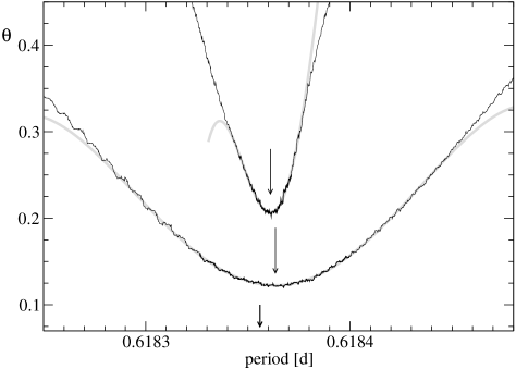
Figure 13: The PDM $\theta$ cores of the $V$ data around the minimum. The thick lines give the results from the data (upper: Honneycutt honey01 (2001); lower: our data). The grey lines are polynomial fits of the minima cores to derive the exact positions. The arrows mark the derived minima and the original period derived by Mennickent & Honeycutt (M_H (1995)).

Figure 14: The PDM diagram of the original data set of Mennickent & Honeycutt (M_H (1995)) covering 1991 to April 1995 only by using the default parameters for the binning by Stellingwerf (pvm (1978)). The original result is indicated at the position of the lowest noise peak.

The period above is supported independently by the $I_{\rm C}$ data giving us a period of 0$\aas@@fstack{d}$6183627 ($=0.06$ seconds less). Using the change of the period $P$

$$P^{2}={{4\pi^{2}a^{3}}\over{\rm G}\,M};\qquad(P+\Delta P)^{2}={{4\pi^{2}\hat{a}^{3}}\over{\rm G}\,(M-\Delta M)}$$ (8)

where $a$ and $\hat{a}$ are the separations before and after the outburst, $M$ the total mass of the system, $\Delta P$ the period change and $\Delta M$ the outburst mass. The conservation of angular momentum gives

$$\begin{array}[]{l}\displaystyle{{a^{2}\over P}\,\,\left[{{M_{\scriptscriptstyle\rm WD}\over\left({{M_{\scriptscriptstyle\rm WD}\over M_{\scriptscriptstyle\rm SE}}+1}\right)^{2}}+{M_{\scriptscriptstyle\rm SE}\over\left({{M_{\scriptscriptstyle\rm SE}\over M_{\scriptscriptstyle\rm WD}}+1}\right)^{2}}}\right]=}\\ \\ \displaystyle{\xi\,{a^{2}\over P}\,\,\left[{{\Delta M\over\left({{M_{\scriptscriptstyle\rm WD}\over M_{\scriptscriptstyle\rm SE}}+1}\right)^{2}}}\right]+}\\ \\ \displaystyle{{\hat{a}^{2}\over P+\Delta P}\,\,\left[{{M_{\scriptscriptstyle\rm WD}-\Delta M\over\left({{M_{\scriptscriptstyle\rm WD}-\Delta M\over M_{\scriptscriptstyle\rm SE}}+1}\right)^{2}}+{M_{\scriptscriptstyle\rm SE}\over\left({{M_{\scriptscriptstyle\rm SE}\over M_{\scriptscriptstyle\rm WD}-\Delta M}+1}\right)^{2}}}\right]}\end{array}$$ (9)

The parameter $\xi\in[0,1]$ refers to the efficiency of the angular momentum transfer to the expelled mass. The two extreme are that the expelled mass carries away its original angular momentum ($\xi=1$) and the opposite case that all angular momentum is transferred and thus kept in the system due to viscosity ($\xi=0$). We use these two cases for the calculated range of mass loss given below. The resulting expelled mass does not depend on the period $P$ within the tested range (100 times the formal error). Also the mass of the secondary (testing $1.2<$M${}_{\scriptscriptstyle\rm SE}<2.5\,\,$M_⊙) does not affect the result. The mass of the WD scales direct proportional to $\Delta M$. As it is known to a 10-15% level, it does not influence $\Delta M$ significantly. The main uncertainties originate from the errors of $\Delta P$ and from the choice of $\xi$. Within a factor of 10 around the determined value we got $\Delta P\propto\Delta M$. This gives us, using the extreme values for $\xi$ and three times the formal error of $\Delta P$

$$\qquad 2.2\times 10^{-6}\,\,{\rm M}_{\odot}\,\,\leq\,\,\Delta M\,\,\leq\,\,5.7\times 10^{-6}\,\,{\rm M}_{\odot}.$$

Hachisu & Kato (HaKa (2001)) obtained $4.7\times 10^{-6}\,\,{\rm M}_{\odot}$ from the thick wind model of the outburst. Assuming the last outburst 60 year ago, our result corresponds to $3.6\times 10^{-8}\,\,{\rm M}_{\odot}/{\rm yr}\,\,\leq\,\,\dot{\rm M}\,\,\leq\,\,9.5\times 10^{-8}\,\,{\rm M}_{\odot}/{\rm yr}$. This corresponds well to the accretion rates of the models during the quiescence phase.

8 Conclusions

The models presented allow us to determine the physical parameters of the system within a very small range. This is mainly achieved by the combination of data from different bands and different epochs what is the main advantage to the work of Hachisu & Kato (HaKa (2001), HaKaII (2002)). The model of the recurrent nova two years after the outburst, when it reached a mean quiescent photometric state still differs significantly from the one of the pre–outburst phase. Even speculative, one may assume that the energy transferred during the outburst, when the secondary was completely enclosed by the WD shell, caused a significant extension over the Roche lobe. This increased the mass transfer to $5.5\times 10^{-8}<\dot{M}<1.5\times 10^{-7}\,\,{\rm M}_{\odot}\,{\rm yr}^{-1}$ in 2001/2002. Thus if the mass transfer rate derived from the pre–outburst phase is used as average, it does not reach up to the accreted mass during the 60 years of quiescence. The mass transfer rate of $\dot{M}\approx 2.5\times 10^{-8}\,\,{\rm M}_{\odot}\,{\rm yr}^{-1}$ derived for 1991-1996 differs from that given by Hachisu & Kato by a factor of four due to the different model of the accreting region. The period shift determined in this paper gives us a good estimate of the expelled mass $2.2\times 10^{-6}<\Delta M<5.7\times 10^{-6}\,\,{\rm M}_{\odot}$. Within the errors (the uncertainty due to the angular momentum carried by the ejected material and the uncertainty of the average mass transfer throughout the 60 years of quiescence) the determined expelled mass corresponds to the accretion. Thus the evolution towards the critical mass of the WD runs rather slow at this evolutionary stage. Assuming a net mass increase of $<10^{-6}$ M_⊙ per outburst leads to a few 10⁷ years to reach the critical mass. On the other hand the evolutionary tracks of the secondary show it at a position with extremely rapid increase of its diameter (about 5  10^-10 R_⊙ yr^-1). Moreover the decrease of the orbit is about 10^-7 R_⊙ per outburst. Thus the mass transfer should increase and may even evolve towards steady hydrogen burning (van den Heuvel et al. vH (1992)). The derived distance and interstellar extinction gives us a somewhat higher luminosity than in the outburst models of Hachisu & Kato (HaKa (2001)). This affects also the considerations in Oka et al. (oka (2002)). Because of our smaller inclination we also see some parts of the disk during the primary minimum and thus it is not necessary to increase the temperature of the SE in 2001 to obtain a higher flux.