High Energy Emission from the Prompt Gamma-Ray Burst

Abstract

We study the synchrotron and synchrotron self-Compton (SSC) emission from internal shocks that are responsible for the prompt $\gamma$-ray emission in Gamma-Ray Bursts (GRBs), and consider the relation between these two components, taking into account the high energy cutoff due to pair production and Thomson scattering. We find that in order for the peak energy of the synchrotron to be $E_{p}\sim 300\;{\rm keV}$ with a variability time $t_{v}\gtrsim 1\;{\rm ms}$, a Lorentz factor of $\Gamma\lesssim 350$ is needed, implying no high energy emission above $\sim 30\;{\rm MeV}$ and the synchrotron component would dominate at all energies. If we want both $E_{p}\sim 300\;{\rm keV}$ and prompt high energy emission up to $\sim 2\;{\rm GeV}$, as detected by EGRET for GRB 940217, we need $\Gamma\sim 600$ and $t_{v}\sim 0.1\;{\rm ms}$, which might be resolved by super AGILE. If such prompt high energy emission is common in GRBs, as may be tested by GLAST, then for $t_{v}\gtrsim 1\;{\rm ms}$ we need $\Gamma\gtrsim 350$, which implies $E_{p}\lesssim 100\;{\rm keV}$. Therefore if X-ray flashes are GRBs with high values of $t_{v}$ and $\Gamma$, they should produce $\gtrsim 1\;$GeV emission. For an electron power law index $p>2$, the SSC component dominates the emission above $\sim 100\;{\rm MeV}$. Future observations by GLAST may help determine the value of $p$ and whether the high energy emission is consistent with a single power law (implying one component–the synchrotron, is dominant) or has a break where the $\nu F_{\nu}$ slope turns from negative to positive, which implies that the SSC component becomes dominant above $\sim 100\;$MeV. The high energy emission is expected to show similar variability and time structure to that of the soft $\gamma$-ray emission. Finally, we find that in order to see delayed high energy emission from the prompt GRB due to pair production with the cosmic IR background, extremely small inter-galactic magnetic fields ($\lesssim 10^{-22}\;{\rm G}$) are required.

1 Introduction

The leading models of Gamma-Ray Bursts (GRBs) involve a relativistic flow emanating from a compact central source, where the prompt gamma-ray emission is attributed to internal shocks within the outflow itself, that arise from variability in its Lorentz factor, while the afterglow results from an external shock that is driven into the ambient medium, as it decelerates the original ejecta (Rees & Mészáros 1994; Sari & Piran 1997). In this so called ‘internal-external’ shock model, the duration of the prompt GRB is directly related to the time during which the central source is active. The most popular emission mechanism is synchrotron radiation from relativistic electrons accelerated in the shocks, that radiate in the strong magnetic fields (close to equipartition values) within the shocked plasma. An additional radiation mechanism that may also play an important role is synchrotron self-Compton (SSC), which is the upscattering of the synchrotron photons by the relativistic electrons, to much higher energies.

The synchrotron and SSC components from internal shocks have been considered in previous works in various contexts. Papathanassiou & M esz aros (1996) studied the emission from internal shocks, focusing on the comparison between internal and external shocks. Pilla & Loeb (1998) calculated the spectrum from internal shocks taking into account multiple Compton scattering and pair production. They show the broad band spectrum for a fixed radius of collision, $R$, and varying Lorentz factor, $\Gamma$, of the outflow, and for a fixed $\Gamma$ and a varying $R$. Our treatment differs in that we assume different free parameters, namely the Lorentz factor $\Gamma$ and the variability time, $t_{v}$ of the central engine that emits the outflow, rather than the $\Gamma$ and $R$. Under our assumptions, the radius of collision scales as $R\sim 2\Gamma^{2}ct_{v}\propto\Gamma^{2}$, and is not independent of $\Gamma$. This results in different conclusions as to the relation between the prompt gamma-ray emission in the BATSE range and the emission at higher energies, which is the main subject of our work. Panaitescu & M esz aros (2000) explored the possibility that the prompt gamma-ray emission in the BATSE range arises from the SSC component rather than the synchrotron, where the latter is in the optical or UV range. Recently, Dai & Lu studied the SSC emission from internal shocks, concentrating on the possible interaction of high energy photons with the IR background (see section §3).

In this Letter we calculate the high energy emission during the prompt GRB from internal shocks, for both the synchrotron and SSC components, and consider the relations between these two components. We estimate the high energy cutoff and study the constraints on the model parameters that arise from the requirement that $E_{p}$ (the typical photon energy of the synchrotron component) will be in the BATSE range.

The synchrotron and SSC spectra are calculated in §2, and expressions are provided for the break frequencies and flux normalization. In §3 we derive the constraints on the model that arise from the optical depth to pair production and to Thomson scattering. We consider the recent claim for a possible delayed emission due to the pair production of high energy photons with the IR background (Dai & Lu 2002) and we show that in order for this radiation to be detectable, a very small ($\lesssim 10^{-22}\;{\rm G}$) inter-galactic magnetic field is needed. Our results are discussed in §4.

2 The Synchrotron and SSC Emission

The Lorentz factor of the flow, $\Gamma$, is assumed to vary on a time scale $t_{v}$ and with a typical amplitude of $\Delta\Gamma\sim\Gamma$. The collisions between the shells typically occur at a radius

$$R\approx 2\Gamma^{2}ct_{v}=6\times 10^{13}\,\Gamma_{2.5}^{2}t_{v,-2}\;{\rm cm}\ ,$$ (1)

where $\Gamma_{2.5}=\Gamma/10^{2.5}$ and $t_{v,-2}=t_{v}/10^{-2}\;{\rm s}$. The internal energy that is released in each collision between shells is distributed among electrons magnetic fields and protons, with fractions $\epsilon_{e}$, $\epsilon_{B}$ and $1-\epsilon_{e}-\epsilon_{B}$, respectively. Since the electrons are typically in the fast cooling regime (as is shown below), the luminosity $L=(\Omega_{j}/4\pi)L_{iso}$ (where $\Omega_{j}$ is the solid of the GRB outflow) of a single pulse, that corresponds to a single collision between two shells within the outflow, is equal to the rate at which energy is given to the electrons by the internal shock. The internal shocks are expected to be at least mildly relativistic, so that we may assume that in the rest frame of the shocked fluid, the velocity of the shock is close to that for a relativistic shock, $c/3$. The local frame luminosity is $L^{\prime}=L/\Gamma^{2}=\Omega_{j}R^{2}\epsilon_{e}e^{\prime}c/3$, and the internal energy density is given by

$$e^{\prime}\approx{3L_{iso}\over 4\pi R^{2}c\Gamma^{2}\epsilon_{e}}=2.2\times 10^{8}\epsilon_{e}^{-1}L_{52}\Gamma_{2.5}^{-6}t_{v,-2}^{-2}\;{\rm erg\;cm^{-3}}\ ,$$ (2)

where $L_{iso}=L_{52}10^{52}\,{\rm erg/s}$. Primed quantities are measured in the local rest frame of the shocked fluid, while un-primed quantities are measured in the observer frame.

For a mildly relativistic shock, the internal energy behind the shock is similar to the rest energy,

$$n^{\prime}\approx{e^{\prime}\over m_{p}c^{2}}\approx{3L_{iso}\over 4\pi R^{2}m_{p}c^{3}\Gamma^{2}\epsilon_{e}}=1.5\times 10^{11}\epsilon_{e}^{-1}L_{52}\Gamma_{2.5}^{-6}t_{v,-2}^{-2}\;{\rm cm^{-3}}\ ,$$ (3)

The magnetic field is

$$B^{\prime}=\sqrt{8\pi\epsilon_{B}e^{\prime}}\approx 7.5\times 10^{4}\epsilon_{e}^{-1/2}\epsilon_{B}^{1/2}L_{52}^{1/2}\Gamma_{2.5}^{-3}t_{v,-2}^{-1}\;{\rm G}\ .$$ (4)

The electrons are accelerated in the shock to a power-law distribution of energies $N(\gamma)=dn^{\prime}/d\gamma\propto\gamma^{-p}$ for $\gamma$ in the range $\gamma_{m}<\gamma<\gamma_{M}$. The minimum Lorentz factor is given by

$$\gamma_{m}=\left({p-2\over p-1}\right){\epsilon_{e}e^{\prime}\over n^{\prime}m_{e}c^{2}}\approx\left({p-2\over p-1}\right){m_{p}\over m_{e}}\,\epsilon_{e}\approx 610f_{p}\,\epsilon_{e}\ .$$ (5)

where $f_{p}\equiv 3(p-2)/(p-1)$.

The electrons radiatively cool by the combination of the synchrotron and SSC processes, the timescales of which are $t^{\prime}_{\rm syn}\sim 6\pi m_{e}c/\sigma_{T}B^{\prime 2}\gamma_{e}$ and $t_{SC}=t_{\rm syn}/Y$,the combined cooling time being $t^{\prime}_{c}=(1/t^{\prime}_{\rm syn}+1/t^{\prime}_{SC})^{-1}=t^{\prime}_{\rm syn}/(1+Y)$, where

$$Y\approx\left\{\matrix{\epsilon_{e}/\epsilon_{B}&\epsilon_{e}\ll\epsilon_{B}\cr&\cr\sqrt{\epsilon_{e}/\epsilon_{B}}&\epsilon_{e}\gg\epsilon_{B}}\right.\ ,$$ (6)

is the Compton y-parameter (Sari, Piran & Narayan 1996). The maximum Lorentz factor of the electrons, $\gamma_{M}$, and the cooling Lorentz factor, $\gamma_{c}$, are set by equating $t^{\prime}_{c}$ with the acceleration time, $\sim 2\pi\gamma_{e}m_{e}c/qB^{\prime}$ (where $q$ is the electric charge of the electron), and the dynamical time, $t^{\prime}_{dyn}=R/c\Gamma\approx 2\Gamma t_{v}$, respectively:

$$\gamma_{M} = \sqrt{3q\over B^{\prime}\sigma_{T}(1+Y)}\approx 1.7\times 10^{5}\,{\epsilon_{e}^{1/4}\Gamma_{2.5}^{3/2}t_{v,-2}^{1/2}\over\sqrt{1+Y}\,\epsilon_{B}^{1/4}L_{52}^{1/4}}\ ,$$ (7)

$$\gamma_{c} = {6\pi\Gamma m_{e}c^{2}\over(1+Y)B^{\prime 2}\sigma_{T}R}\approx 0.02\,{\epsilon_{e}\Gamma_{2.5}^{5}t_{v,-2}\over(1+Y)\epsilon_{B}L_{52}}\ .$$ (8)

Obviously, $\gamma_{c}<1$ no longer corresponds to the Lorentz factor of the electrons, and instead represents the fraction of the dynamical time (the shell shock crossing time for internal shocks) during which the electrons cool to a non-relativistic random Lorentz factor. In this case, the electrons are relativistic only within a thin layer behind the shock, of width $\gamma_{c}\Delta^{\prime}$, where $\Delta^{\prime}$ is the width of the shell, and are cold (i.e. non-relativistic) in the rest of the shell. As can be seen from equations (5) and (8), typically $\gamma_{c}\ll\gamma_{m}$ and the electrons are fast cooling.

The synchrotron frequency and the total synchrotron power of a single electron are given by

$$\nu_{syn}=\nu_{0}\gamma_{e}^{2}=\Gamma\,{3q_{e}B^{\prime}\gamma_{e}^{2}\over 16m_{e}c}\quad,\quad P_{e,syn}=\Gamma^{2}{4\over 3}\sigma_{T}c{B^{\prime 2}\over 8\pi}\gamma_{e}^{2}\ ,$$ (9)

where $\nu^{\prime}_{syn}=\nu_{syn}/\Gamma$ and $P^{\prime}_{e,syn}=P_{e,syn}/\Gamma^{2}$. The self absorption frequency is typically ${\rm max}(\nu_{c},\nu_{0})<\nu_{sa}<\nu_{m}$, and the absorption coefficient is given by

$$\alpha^{\prime}_{\nu}\approx{3\gamma_{c}n^{\prime}(P^{\prime}_{e,syn}/\nu^{\prime}_{syn})\over 16\pi m_{e}\nu^{5/3}\nu_{b0}^{1/3}}\left(\frac{16m_{e}c\nu}{3qB_{b}}\right)^{-4/3}\ .$$ (10)

We solve $\alpha^{\prime}_{\nu^{\prime}_{sa}}\Delta^{\prime}=1$ for $\nu^{\prime}_{sa}$, where $\Delta^{\prime}\approx R/\Gamma$ is the width of the shell in the local frame, and then we have $\nu_{sa}=\Gamma\nu^{\prime}_{sa}$. The synchrotron frequencies are given by

$$\nu_{c} = 3.7\times 10^{10}\,(1+Y)^{-2}\epsilon_{e}^{3/2}\epsilon_{B}^{-3/2}L_{52}^{-3/2}\Gamma_{2.5}^{8}t_{v,-2}\;{\rm Hz}\ ,$$

$$\nu_{0} = 7.8\times 10^{13}\,\epsilon_{e}^{-1/2}\epsilon_{B}^{1/2}L_{52}^{1/2}\Gamma_{2.5}^{-2}t_{v,-2}^{-1}\;{\rm Hz}\ ,$$

$$\nu_{ac} = 5.7\times 10^{13}f_{p}^{-8/5}(1+Y)^{-3/5}\epsilon_{e}^{-9/5}\epsilon_{B}^{-2/5}L_{52}^{1/5}\Gamma_{2.5}^{-1/5}t_{v,-2}^{-2/5}\;{\rm Hz}\ ,$$

$$\nu_{sa} = 2.0\times 10^{16}\,(1+Y)^{-1/3}\epsilon_{e}^{-1/3}L_{52}^{1/3}\Gamma_{2.5}^{-1}t_{v,-2}^{-2/3}\;{\rm Hz}\ ,$$ (11)

$$\nu_{m} = 2.9\times 10^{19}\,f_{p}^{2}(1+Y)^{-1/3}\epsilon_{e}^{3/2}\epsilon_{B}^{1/2}L_{52}^{1/2}\Gamma_{2.5}^{-2}t_{v,-2}^{-1}\;{\rm Hz}\ ,$$

$$\nu_{M} = 2.3\times 10^{24}\,(1+Y)^{-1}\Gamma_{2.5}\;{\rm Hz}\ ,$$

and the synchrotron spectrum is

$${\nu F_{\nu}\over\nu_{m}F_{\nu_{m}}}=\left\{\matrix{(\nu_{sa}/\nu_{m})^{1/2}(\nu_{ac}/\nu_{sa})^{19/8}(\nu/\nu_{ac})^{3}&\ \ \nu<\nu_{ac}\cr&\cr(\nu_{sa}/\nu_{m})^{1/2}(\nu/\nu_{sa})^{19/8}&\ \ \nu_{ac}<\nu<\nu_{sa}\cr&\cr(\nu/\nu_{m})^{1/2}&\nu_{sa}<\nu<\nu_{m}\cr&\cr(\nu/\nu_{m})^{(2-p)/2}&\nu_{m}<\nu<\nu_{M}}\right.\ ,$$ (12)

where from the normalization condition we obtain,

$${L_{iso}\over 4\pi D^{2}} = \int_{0}^{\infty}d\nu F_{\nu}=6f_{p}^{-1}\nu_{m}F_{\nu_{m}}\ ,$$ (13)

$$\nu_{m}F_{\nu_{m}} = {f_{p}L_{iso}\over 24\pi D^{2}}=1.3\times 10^{-6}f_{p}L_{52}D_{28}^{-2}\;{\rm erg\,\,cm^{-2}\,s^{-1}}\ ,$$ (14)

where $D=10^{28}D_{28}\;{\rm cm}$ is the distance to the GRB.

The SSC spectrum is given by

$${\nu F_{\nu}^{SC}\over Y\nu_{m}F_{\nu_{m}}}=\left\{\matrix{(\nu_{sa}^{SC}/\nu_{m}^{SC})^{1/2}(\nu/\nu_{sa}^{SC})^{2}&\ \ \nu<\nu_{sa}^{SC}\cr&\cr(\nu/\nu_{m}^{SC})^{1/2}&\nu_{sa}^{SC}<\nu<\nu_{m}^{SC}\cr&\cr(\nu/\nu_{m}^{SC})^{(2-p)/2}&\nu_{m}^{SC}<\nu<\nu_{KN}^{SC}\cr&\cr(\nu_{KN}^{SC}/\nu_{m}^{SC})^{2-p\over 2}(\nu/\nu_{KN}^{SC})^{1-2p\over 2}&\nu_{KN}^{SC}<\nu<\nu_{M}^{SC}\cr&\cr}\right.\ ,$$ (15)

where $\nu_{sa}^{SC}\equiv\max(\gamma_{c}^{2},1)\nu_{sa}$ and

$$\nu_{m}^{SC} = \gamma_{m}^{2}\nu_{m}=1.1\times 10^{25}f_{p}^{4}\epsilon_{e}^{7/2}\epsilon_{B}^{1/2}L_{52}^{1/2}\Gamma_{2.5}^{-2}t_{v,-2}^{-1}\;{\rm Hz}\ ,$$

$$\nu_{KN}^{SC} = \Gamma^{2}m_{e}^{2}c^{4}/h^{2}\nu_{m}=5.2\times 10^{25}f_{p}^{-2}\epsilon_{e}^{-3/2}\epsilon_{B}^{-1/2}L_{52}^{-1/2}\Gamma_{2.5}^{4}t_{v,-2}\;{\rm Hz}\ ,$$ (16)

$$\nu_{M}^{SC} = \Gamma\gamma_{M}m_{e}c^{2}/h=6.6\times 10^{27}(1+Y)^{-1/2}\epsilon_{e}^{1/4}\epsilon_{B}^{-1/4}L_{52}^{-1/4}\Gamma_{2.5}^{5/2}t_{v,-2}^{1/2}\;{\rm Hz}\ .$$

If $\nu_{KN}^{SC}<\nu_{m}^{SC}$ then we have $\nu F_{\nu}\propto\nu^{1/2-p}$ for $\nu_{KN}^{SC}<\nu<\nu_{M}^{SC}$. For details about the spectrum above the Klein-Nishina frequency, $\nu_{KN}^{SC}$, see Guetta & Granot (2002).

3 The High Energy Cutoff

In order for high energy photons to escape the system and reach the observer, they must overcome a few potential obstacles along the way. Inside the source, there are two main constraints: i) the opacity of the high energy photons to pair production due to interaction with lower energy photon, $\tau_{\gamma\gamma}$, must be smaller than 1 in order for high energy photons to escape, and ii) the Thomson optical depth due to pair production, $\tau_{p}$, must be smaller than unity in order for the observed prompt GRB emission to escape and reach the observer. These effects have been studied by several different authors (Sari & Piran 1997; Lithwick & Sari 2001; Guetta, Spada & Waxman 2001). Outside of the source, high energy photons ($\gtrsim 500\;$GeV) may interact with photons from the cosmic IR background to produce pairs (Salamon & Stecker 1998; Dai & Lu 2002).

We reparameterize the expressions of Lithwick & Sari (2001) for $\tau_{\gamma\gamma}$ and $\tau_{p}$, using our parameters, and express the requirements $\tau_{\gamma\gamma}<1$ and $\tau_{p}<1$ as constraints on the Lorentz factor $\Gamma$:

$$\Gamma > 69\,\epsilon_{e}^{3(p-2)\over 8(p+1)}\epsilon_{B}^{(p-2)\over 8(p+1)}L_{52}^{(p+2)\over 8(p+1)}t_{v,-2}^{-{p\over 4(p+1)}}\varepsilon_{\rm max}^{{p\over 4(p+1)}}\quad(\tau_{\gamma\gamma}<1)\ ,$$ (17)

$$\Gamma > 170\,\epsilon_{e}^{3(p-2)\over 2(3p+4)}\epsilon_{B}^{(p-2)\over 2(3p+4)}L_{52}^{(p+2)\over 2(3p+4)}t_{v,-2}^{(p+2)\over(3p+4)}\quad\quad\ \ (\tau_{p}<1)\ ,$$ (18)

where $\varepsilon_{\rm max}$ is the maximal energy of a photon that can escape (measured in the observer frame, in units of $m_{e}c^{2}$) and the numerical coefficients are for $p=2.5$, but do not vary by more than $10\%$ for $2.05<p<2.9$. In order to see the soft gamma-rays from the prompt GRB, the inequality in Eq. (18) must be satisfied, in which case there will be an upper cutoff at

$$h\nu_{\gamma\gamma}\equiv\varepsilon_{\rm max}m_{e}c^{2}=2.6\,\epsilon_{e}^{-3(p-2)\over 2p}\epsilon_{B}^{(2-p)\over 2p}L_{52}^{-{(p+2)\over 2p}}\Gamma_{2.5}^{4(p+1)\over p}t_{v,-2}\;{\rm GeV}\ ,$$ (19)

where the numerical coefficient is for $p=2.5$ and varies by less than $10\%$ for $2.17<p<2.67$. The maximum photon energy detected by EGRET during the prompt emission is $\sim 3$ GeV (Hurley et al. 1994), for which Eq. (17) implies $\Gamma>370$ for our fiducial parameters.

In Figure 1 we show the synchrotron and SSC $\nu F_{\nu}$ spectra, for different values of $\Gamma$ and $t_{v}$. As can be seen from this figure, the high energy cutoff is typically determined by the opacity to pair production, and is given by Eq. (19). As mentioned above, the high energy photons ($\gtrsim 500\;{\rm GeV}$) that escape the source may still interact with the cosmic IR background and produce pairs. However, as illustrated in Figure 1, in order for photons in this energy range to leave the system, one needs $\Gamma\gtrsim 600$ and $t_{v}\gtrsim 0.01\;{\rm s}$, which, in turn, implies $h\nu_{m}=E_{p}\lesssim 1\;{\rm keV}$. Therefore, this effect is expected to be irrelevant for typical GRBs, with $E_{p}$ in the BATSE range, and might play a role only for the low end of the $E_{p}$ distribution of the X-ray flashes.

It has recently been claimed (Dai & Lu 2002) that a delayed emission on a timescale of $\Delta t\sim 10^{3}\;{\rm sec}$ after the GRB may result due to the inverse Compton upscattering of the CMB by the pairs produced by photons with energies $\gtrsim 300\;{\rm GeV}$ that are emitted during the prompt GRB, with the cosmic IR background. The pairs are produced at a typical distance of $R_{pair}\approx 5.8\times 10^{24}\;{\rm cm}$, and loose their energy by upscattering CMB photons over a length scale of $R_{IC}\approx 7.3\times 10^{24}\;{\rm cm}$. Dai & Lu estimated the delay time by $\Delta t\sim R/2\gamma_{e}^{2}$, where $R=\max(R_{pair},R_{IC})$. This estimate is based on the fact that the pairs that are produced initially propagate almost in the same direction as the high energy photon (i.e. in the radial direction from the GRB) and on the assumption that they do not change their direction by more than $1/\gamma_{e}$ over $R_{IC}$. However, the presence of intergalactic magnetic fields (IGMF), $B_{IG}$, at $R_{pair}$ will cause a deflection angle of

$$\theta_{\rm def}={R_{IC}\over R_{L}}=1.4\times 10^{5}\left({B_{IG}\over 10^{-11}\,{\rm G}}\right)\left({\gamma_{e}\over 3\times 10^{5}}\right)^{-2}\ ,$$ (20)

where $R_{L}=\gamma_{e}m_{e}c^{2}/qB$ is the Larmor radius of the electron. In order for the above estimate for $\Delta t$ not to be effected by this deflection, we need $\theta_{\rm def}<1/\gamma_{e}$, which according to Eq. (20) implies $B_{IG}<B_{0}=2.3\times 10^{-22}\;{\rm G}$. For $B_{IG}>B_{0}$, the value of $\Delta t$ increases by a factor of $\sim(B_{IG}/B_{0})^{2}$ compared to the estimate of Dai & Lu. For $\theta_{\rm def}>1$, i.e. $B_{IG}\gtrsim 10^{-16}\;{\rm G}$, we expect $\Delta t\sim R_{IC}/c\sim 10^{7}\;{\rm yr}$, and a roughly isotropic emission. Therefore, the detection of such a delayed emission will suggest an IGMF $\lesssim 10^{-21}\;$G at a distance of a few Mpc from the site of the GRB, while the lack of detection of this emission will imply a larger IGMF. As in such a distance from the site of the GRB one typically expects to reach a void, this can serve as a mothod for estimating the highly uncertain value of the IGMF in voids. A similar suggestion was made by Plaga (1995).

4 Discussion

We have calculated the synchrotron and SSC emission during the prompt GRB from internal shocks, and studied the relation between these two components and its dependence on the model parameters. Our analysis takes into account the high energy cutoffs due to the Klein-Nishina effect, pair production with low energy photons and with the cosmic IR background, and Thomson scattering.

For $p>2$ the emission above $\sim 100\;{\rm MeV}$, is typically dominated by the SSC emission, while the synchrotron component is dominant at lower energies. If the variability time is $t_{v}\gtrsim 1\;{\rm ms}$, then $E_{p}\sim 300\;{\rm keV}$ would imply a cutoff at $\sim 30\;{\rm MeV}$, and the synchrotron emission would be dominant at all energies. Future observations by GLAST may help determine the value of $p$ and whether the high energy emission is consistent with a single power law or has a break where the $\nu F_{\nu}$ slope turns from negative to positive. The former would imply that the high energy emission is dominated by a single component– the synchrotron emission, while the latter implies that the SSC component becomes dominant above a certain energy ($\sim 100\;$MeV).

The SSC high energy emission should show a similar variability to that observed in the BATSE range. An additional emission mechanism that might contribute to the high energy emission, is external Compton, which may be relevant if GRBs occur inside pulsar wind bubbles (Guetta & Granot 2002).

In addition, there might be delayed high energy emission from the internal shocks, due to upscattering, aas was suggested by of the CMB by $e^{\pm}$ pairs produced by the interaction between $\gtrsim 300\;$GeV photons from the prompt GRB with the IR background photons (Dai & Lu 2002). The detection of such emission would be possible only for inter galactic magnetic fields (IGMF) $\lesssim 10^{-21}\;$G at a distance of a few Mpc from the site of the GRB, so that it may serve a probe for the strength of the IGMF in voids.

As can be seen from Eqs. (2), (19) and Figure 1, larger values of $\Gamma$ or $t_{v}$ shift the cutoff at $h\nu_{\gamma\gamma}$ to larger energies, while at the same time, it implies lower values of $E_{p}$. For example, in order to have $\sim 1\;{\rm GeV}$ photons for $t_{v}\sim 1\;{\rm ms}$ we need $\Gamma\gtrsim 350$, which in turn, imply $E_{p}\lesssim 100\;{\rm keV}$. If X-ray flashes are GRBs with such parameters, as suggested by Guetta, Spada & Waxman (2001), then we can expect GeV emission from X-ray flashes.

In order to explain the prompt high energy photons, of up to $\sim 3\;{\rm GeV}$, that were observed in GRB 940217 (Hurley et al. 1994), together with the value of $E_{p}\approx 200\;{\rm keV}$ that was measured for this burst, we need a very small variability time $t_{v}\sim 0.1\;{\rm ms}$, and $\Gamma\sim 600$ (see the solid curve in the lower panel of Figure 1). If indeed such high energy emission is typical for GRBs with $E_{p}$ in the BATSE range, as can be tested by the future mission GLAST, this might suggest very low variability times ($t_{v}\lesssim 0.1\;{\rm ms}$). This possibility is consistent with the fact that in many GRBs the shortest measured variability time is limited by the temporal resolution of the instrument, and there is no observational lower limit on $t_{v}$. On the other hand, $t_{v}\sim 0.1\;{\rm ms}$ implies a source size $\lesssim ct_{v}\sim 30\,t_{v,-4}\;{\rm Km}$, so that it is unlikely that $t_{v}$ can be much smaller that $0.1\;{\rm ms}$. Therefore, this might imply a typical variability time of $t_{v}\sim 0.1\;{\rm ms}$, which may be resolved by super AGILE.

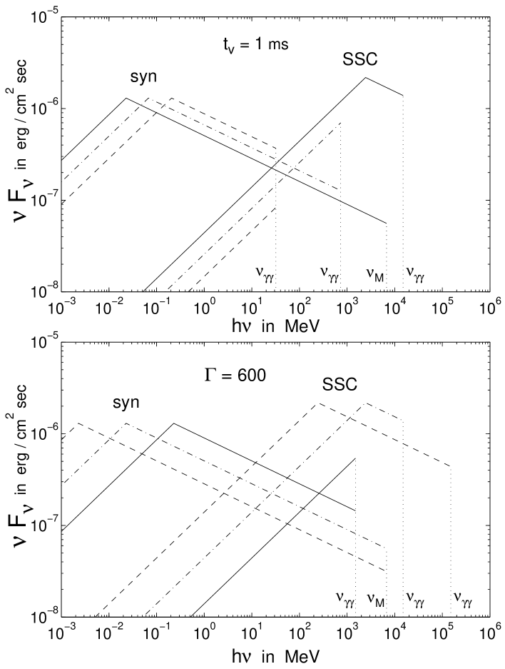
Figure 1: The $\nu F_{\nu}$ spectrum from the prompt GRB for the synchrotron and SSC components, including the relevant high energy cutoff among the possibilities discussed in the text. In the upper panel we fix $t_{v}=1\;{\rm ms}$, and the dashed, dashed-dotted and solid lines correspond to $\Gamma=200,\,350$ and $600$, respectively. In the lower panel we fix $\Gamma=600$, and the dashed, dashed-dotted and solid lines correspond to $t_{v}=10,\,1$ and $0.1\;{\rm ms}$, respectively. In both panels we use $L_{52}=1$ and $p=2.5$, as well as $\epsilon_{e}=0.45$ and $\epsilon_{B}=0.1$, where the latter were chosen so that the peak of $\nu F_{\nu}$ of the synchrotron would be at the right range (Guetta, Spada & Waxman 2001).

References

• Dai & Lu (2002) Dai, Z.G., & Lu, T. 2002, accepted to ApJ (astro-ph/0203084)
• Granot, Piran, & Sari (2000) Granot, J., Piran, T. & Sari, R. 2000, ApJ, 534, L163
• Guetta & Granot (2002) Guetta, D., & Granot, J. 2002, submitted to MNRAS (astro-ph/0208156)
• Guetta, Spada & Waxman (2001) Guetta, D., Spada, M., & Waxman, E. 2001, ApJ, 557, 399
• Hurley et al. (1994) Hurley, K., et al. 1994, Nature, 372, 652
• Lithwick & Sari (2001) Lithwick, Y., & Sari, R. 2001, ApJ, 555, 540
• Panaitescu & M esz aros (2000) Panaitescu, A., & M esz aros, P. 2000, ApJ, 544, L17
• Papathanassiou & M esz aros (1996) Papathanassiou, H., & M esz aros, P. 1996, ApJ, 471, L91
• Pilla & Loeb (1998) Pilla, R.P., & Loeb, A. 1998, ApJ, 494, L167
• Plaga (1995) Plaga, R., 1995, Nature 374, 430
• Rees & MΓ©szΓ‘ros (1994) Rees, M. J., & MΓ©szΓ‘ros, P. 1994, ApJ, 430, L93
• Salamon & Stecker (1998) Salamon, M.H., & Stecker, F.W. 1998, ApJ, 493, 547
• Sari & Piran (1997) Sari, R., & Piran, T. 1997, MNRAS, 287, 110
• Sari, Piran & Narayan (1996) Sari, R., Piran, T., & Narayan, R. 1996, ApJ, 473, 204
Refer to caption