CMB Anisotropy Constraints on Flat-$\Lambda$ and Open CDM Cosmogonies from DMR, UCSB South Pole, Python, ARGO, MAX, White Dish, OVRO, and SuZIE Data

Abstract

We use joint likelihood analyses of combinations of fifteen cosmic microwave background (CMB) anisotropy data sets from the DMR, UCSB South Pole 1994, Python I–III, ARGO, MAX 4 and 5, White Dish, OVRO, and SuZIE experiments to constrain cosmogonies. We consider open and spatially-flat-$\Lambda$ cold dark matter cosmogonies, with nonrelativistic-mass density parameter $\Omega_{0}$ in the range 0.1–1, baryonic-mass density parameter $\Omega_{B}$ in the range (0.005–0.029)$h^{-2}$, and age of the universe $t_{0}$ in the range (10–20) Gyr.

Marginalizing over all parameters but $\Omega_{0}$, the data favor $\Omega_{0}\simeq$ 0.9–1 (0.4–0.6) flat-$\Lambda$ (open) models. The range in deduced $\Omega_{0}$ values is partially a consequence of the different combinations of smaller-angular-scale CMB anisotropy data sets used in the analyses, but more significantly a consequence of whether the DMR quadrupole moment is accounted for or ignored in the analysis. While the open model is difficult to reconcile with the results of less exact analyses of more recent CMB anisotropy data, the lower values of $\Omega_{0}$ found in this case are more easily reconciled with dynamical estimates of this parameter. For both flat-$\Lambda$ and open models, after marginalizing over all other parameters, a lower $\Omega_{B}h^{2}\simeq$ 0.005–0.009 is favored. This is also marginally at odds with estimates from more recent CMB anisotropy data and some estimates from standard nucleosynthesis theory and observed light element abundances. For both sets of models a younger universe with $t_{0}\simeq$ 12–15 Gyr is favored, consistent with other recent non-CMB indicators. We emphasize that since we consider only a small number of data sets, these results are tentative. More importantly, the analyses here do not rule out the currently favored flat-$\Lambda$ model with $\Omega_{0}\sim 0.3$, nor the larger $\Omega_{B}h^{2}$ values favored by some other data.

1 Introduction

There has been a remarkable increase in the quality and quantity of cosmic microwave background (CMB) anisotropy measurements since the initial detection of the anisotropy on large angular scales a decade ago. These measurements are becoming increasingly useful in the continuing processes of determining how well cosmological models approximate reality and for constraining cosmological parameters such as $\Omega_{0}$, $h$, and $\Omega_{B}$ in these models.

In this paper we utilize the full information in the data from each experiment in an effort to place robust constraints on cosmological parameters. This is achieved through a maximum likelihood analysis of the data using realistic model anisotropy spectra. Most of the data sets we consider in this paper are small, in contrast to some of the more recent data sets (see, e.g., Netterfield et al. 2002; Stompor et al. 2001), which because of their size require a more approximate analysis technique. Ganga et al. (1997a, hereafter GRGS) extend the maximum likelihood technique to account for uncertainties, such as those in the beamwidth of the telescope and the calibration of the experiment. This technique has been used with model CMB anisotropy spectra in analyses of the Gundersen et al. (1995) UCSB South Pole 1994 data, the Church et al. (1997) SuZIE data, the Lim et al. (1996) MAX 4+5 data, the Tucker et al. (1993) White Dish data, the de Bernardis et al. (1994) ARGO data, the Platt et al. (1997) Python I–III data, and the Leitch et al. (2000) OVRO data (GRGS; Ganga et al. 1997b, 1998; Ratra et al. 1998, 1999a, hereafter R99a; Rocha et al. 1999; Mukherjee et al. 2002b).

Given the error bars associated with these measurements, interesting constraints on cosmological model parameters require the joint analysis of many data sets. If the measurements are acquired for regions well separated in space, or on very different angular scales, the likelihoods of the individual data sets are independent and can thus be multiplied together to construct the likelihood of the combined data set. This combined likelihood is then used to derive constraints on cosmological model parameters. A combined analysis of the smaller-angular-scale data sets listed above, excluding the Python and OVRO data, is presented in Ratra et al. (1999b, hereafter R99b). In this paper we extend the analysis of R99b to include the Python and OVRO data, as well as the large angular scale DMR data (Górski et al. 1998, hereafter G98; Stompor 1997).

In $\S$ 2 we describe the models and cosmological parameter space we consider. See R99a for a more detailed description. In $\S$ 3 we summarize the various combinations of data sets we consider. See R99b for further details. In $\S$ 4 we summarize the computational techniques we use. See GRGS and R99b for more detailed discussions. In $\S$ 5 we present and discuss results from analyses of various combinations of the smaller-angular-scale CMB anisotropy data sets, and in $\S$ 6 we add the DMR data to the mix. We conclude in $\S$ 7.

2 Cosmogonical Models

In this paper we focus on a spatially-flat cold dark matter (CDM) model with a cosmological constant $\Lambda$. This model is consistent with most current measurements. While it is important to compare the currently favored model to the CMB anisotropy data, it is also important to check how well other, currently less favored, models fare. We therefore also examine the constraints these data place on a spatially-open model with no $\Lambda$ (see, e.g., Gott 1982; Ratra & Peebles 1995). For more detailed discussions of these models see R99a and R99b.

The CMB anisotropy spectra in these models are generated as quantum fluctuations in a weakly coupled field during an early epoch of inflation. They are thus realizations of spatially stationary Gaussian random processes (see, e.g., Ratra 1985; Fischler, Ratra, & Susskind 1985). The measured CMB anisotropy appears to be consistent with this Gaussianity assumption (see, e.g., Mukherjee, Hobson, & Lasenby 2000; Park et al. 2001; Wu et al. 2001; Shandarin et al. 2002; Santos et al. 2002; Komatsu et al. 2002; Polenta et al. 2002), and the experimental noise also appears to be Gaussian, thus validating our use of the likelihood analysis method of GRGS.

To make the computations tractable, in each model (flat-$\Lambda$ and open) we consider CMB anisotropy spectra parameterized by (i) the quadrupole-moment amplitude $Q_{\rm rms-PS}$, (ii) $\Omega_{0}$, (iii) $\Omega_{B}h^{2}$, and (iv) $t_{0}$. While it is of interest to also consider other cosmological parameters current data do not require consideration of a larger dimensional parameter space. That is, current data appear to indicate that effects like reionization and tilt and those due to primordial gravity waves are small. Furthermore, the maximum likelihood analysis technique used here is computationally intensive and an analysis that takes account of more cosmological parameters will be very time consuming. Rather than make approximations (e.g., data compression) to speed up such a computation and minimize memory requirements, in this paper we perform as accurate a computation as possible based on model spectra from an as small as viable yet still realistic cosmological parameter space.

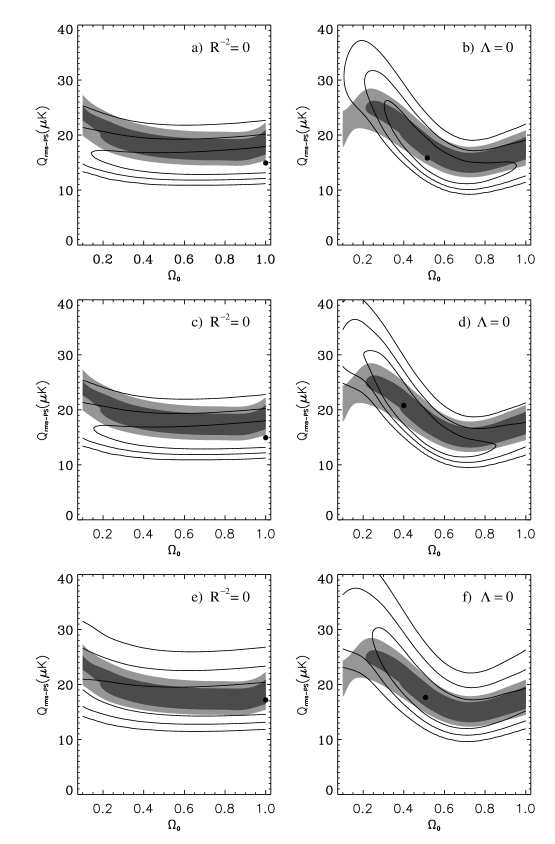
Figure 2: Confidence contours and maxima of the marginalized two-dimensional $(Q_{\rm rms-PS},\Omega_{0})$ posterior probability density distribution functions. Panels $a)$, $c)$, & $e)$ in the left column show the flat-$\Lambda$ model and panels $b)$, $d)$, & $f)$ in the right column show the open model. Lines show the two-dimensional posterior probability density distribution function 1, 2, and 3 $\sigma$ confidence limits derived from the various combination smaller-angular-scale data sets considered. Solid circles show the maxima of the two-dimensional posterior distributions. Shaded regions show the two-dimensional posterior probability density distribution function confidence limits for the DMR data (G98; Stompor 1997); densest shading shows the 1 $\sigma$ confidence region and less-dense shading shows the 2 $\sigma$ region. The DMR results are a composite of those from analyses of the two extreme data sets: i) galactic frame with quadrupole included and correcting for faint high-latitude galactic emission; and ii) ecliptic frame with quadrupole excluded and no other galactic emission correction (G98). Panels $a)$ & $b)$ in the top row are from an analysis of all the small scale data. Panels $c)$ & $d)$ in the middle row are from an analysis of all but the SuZIE small scale data. Panels $e)$ & $f)$ in the bottom row are from an analysis of the SP94Ka, Python I-III, MAX 4 ID, MAX 5 HR, and OVRO data sets.

The CMB anisotropy spectra we use are computed for a range of $\Omega_{0}$ spanning the interval 0.1 to 1 in steps of 0.1, for a range of $\Omega_{B}h^{2}$ spanning the interval 0.005 to 0.029 in steps of 0.004, and for a range of $t_{0}$ spanning the interval 10 to 20 Gyr in steps of 2 Gyr. In total 798 spectra are computed to cover the cosmological-parameter spaces of the open and flat-$\Lambda$ models. Examples of spectra are shown in Fig. 2 of R99a, Fig. 1 of R99b, and Fig. 2 of Rocha et al. (1999).

3 CMB Anisotropy Data Sets

R99b consider various combinations of ten different data sets. These were the UCSB South Pole 1994 Ka and Q band observations, hereafter SP94Ka and SP94Q (Gundersen et al. 1995; GRGS), the ARGO Hercules observations (de Bernardis et al. 1994; R99a), the MAX 4 $\iota$ Draconis (ID) and $\sigma$ Herculis (SH) and MAX 5 HR5127 (HR), $\mu$ Pegasi (MP), and $\phi$ Herculis (PH) observations (Lim et al. 1996; Ganga et al. 1998), the White Dish observations (Tucker et al. 1993; Ratra et al. 1998), and the SuZIE observations (Church et al. 1997; Ganga et al. 1997b). Detailed information about these data sets may be found in the papers cited above and in R99b.

In this paper we augment the data sets used in R99b with the Python I–III data (Platt et al. 1997; Rocha et al. 1999), the OVRO data (Leitch et al. 2000; Mukherjee et al. 2002b), and the DMR data (Bennett et al. 1996; G98; Stompor 1997). This adds an additional five CMB anisotropy data sets to the ten considered in R99b.

R99b consider three different combinations of the CMB anisotropy data sets. The first combination included all data (SP94, ARGO, MAX 4 and 5, White Dish, and SuZIE). The second combination excluded the SuZIE data, which probe the smallest angular scales (to multipole index $l\sim 2000$ in some models, Ganga et al. 1997b), since our model CMB anisotropy spectra do not account for effects that could be important on these small angular scales. The third combination of data used in R99b include just the measurements of SP94Ka, MAX 4 ID, and MAX 5 HR which are thought to provide the most reliable constraints, among the data considered in R99b (see discussion in R99b), to constrain the parameters of the theoretical CMB anisotropy spectra considered in that paper.

The new smaller-angular-scale data used in this paper, Python I–III and OVRO, raise no obvious red flags: we have no reason to think that they are any less reliable than the data considered to be the most reliable in R99b. We therefore again derive cosmological constraints for three different combination CMB anisotropy data sets, augmenting each of the three combination data sets of R99b with the Python I–III and OVRO data.

The situation with the largest angular scale CMB anisotropy data, that measured by the DMR experiment (Bennett et al. 1996; G98), is more complicated. While a couple of other issues also need to be considered, the main complication arises from the effect on the derived cosmological constraints from the inclusion or exclusion of the observed DMR quadrupole moment (Kogut et al. 1996) in the analysis (G98; Stompor 1997). Non-CMB anisotropy emission from the Milky Way is predominantly quadrupolar, and any post-correction remnant of this will primarily affect the observed DMR quadrupole moment. To be sure, this is only of order a 1 $\sigma$ effect on cosmological parameter determination from the DMR data alone. However, given the differences in the constraints derived from the different combinations of smaller-angular-scale data sets we consider (and again, these differences are of order 1 $\sigma$), folding in the DMR data results in more significant differences between cosmological constraints derived using the various combination data sets. One might hope that better maps of foreground emission will help resolve the DMR quadrupole moment issue, but that is for the future. The only option at present appears to be to consider cosmological constraints that follow on using all “reasonable” combinations of data. To illustrate the situation we consider the two most extreme DMR data combinations (G98): (i) the galactic frame data including the quadrupole moment and correcting for faint high-latitude galactic emission (this results in the smallest $Q_{\rm rms-PS}$ value); and (ii) the ecliptic frame data with the quadrupole moment excluded and no other galactic emission correction (this results in the largest $Q_{\rm rms-PS}$ value). In conjunction with the three different combinations of smaller-angular-scale data, these two DMR data sets result in six different combinations of CMB anisotropy data we consider in this paper.

4 Summary of Computation

GRGS describe the computation of the likelihood function for a given CMB anisotropy data set. Offsets and gradients removed from the data are accounted for in the analysis. Beamwidth and calibration uncertainties are also accounted for as described in GRGS. In some cases non-CMB anisotropy foreground contamination have also been accounted for.

The data sets considered in this analysis were acquired from regions well separated in space, or are at very different angular resolution. Consequently they are statistically independent and the likelihood functions of the individual data sets are simply multiplied together to construct the likelihood function of the combined data. The flat-$\Lambda$ and open model likelihoods we consider are a function of the four parameters described in $\S$ 2: $Q_{\rm rms-PS}$, $\Omega_{0}$, $\Omega_{B}h^{2}$, and $t_{0}$. Marginalized likelihood functions are derived by integrating over one or more of these parameters. We assume a uniform prior in the parameters integrated over, set to zero outside the parameter range considered.

To determine central values and limits from the likelihood functions we assume a uniform prior in the relevant parameter. Then the corresponding posterior probability density distribution function vanishes outside the chosen parameter range and is equal to the likelihood function inside this range. The deduced central value of the parameter is taken to be the value at which the posterior probability density peaks, and we quote highest posterior density limits. See GRGS, R99a, and R99b for details. The quoted limits depend on the prior range considered for the parameter. This is a significant effect if the likelihood function is not sharply peaked within the parameter range considered, as is the case for a number of the likelihood functions derived in this paper. See R99a and R99b for more detailed discussions of this issue. In what follows we consider 1, 2, and 3 $\sigma$ highest posterior density limits which include 68.3, 95.4, and 99.7% of the probability.

Rocha et al. (1999) and Mukherjee et al. (2002b) note that the four-dimensional posterior probability density distribution function $L(Q_{\rm rms-PS},\Omega_{0},\Omega_{B}h^{2},t_{0})$ is nicely peaked in the $Q_{\rm rms-PS}$ direction but fairly flat in the other three directions. Marginalizing over $Q_{\rm rms-PS}$ results in a three-dimensional posterior distribution $L(\Omega_{0},\Omega_{B}h^{2},t_{0})$ which is steeper, but still relatively flat. As a consequence, limits derived from the four- and three-dimensional posterior distributions are generally not highly statistically significant. We therefore do not show contour plots of these functions here. Marginalizing over $Q_{\rm rms-PS}$ and one other parameter results in two-dimensional posterior probability distributions which are more peaked. See Fig. 1 for examples of the constraints from the two-dimensional posterior probability distribution functions. As in the ARGO (R99a), Python I–III (Rocha et al. 1999), OVRO (Mukherjee et al. 2002b), and earlier combination (R99b) data set analyses, in some cases these peaks are at an edge of the parameter range considered.

5 Smaller Angular Scale Data: Results and Discussion

Figure 1 shows that even just using the smaller angular scale CMB anisotropy data, the two-dimensional posterior distributions allow one to distinguish between different regions of parameter space at a fairly high formal level of confidence. For instance, for the SP94Ka, Python I–III, MAX 4 ID, MAX 5 HR, and OVRO data combination (panels $c$ and $f$ in the bottom row of Fig. 1), the flat-$\Lambda$ model near $\Omega_{0}\sim 0.1$, $\Omega_{B}h^{2}\sim 0.03$, and $t_{0}\sim 10$ Gyr, is formally ruled out at $\sim 3$ $\sigma$ confidence. However, we emphasize, as discussed in Mukherjee et al. (2002b), care must be exercised when interpreting the discriminative power of these formal limits, since they depend sensitively on the fact that the uniform prior has been set to zero outside the range of the parameter space we have considered.

Figure 2 shows the contours of the two-dimensional posterior distribution for $Q_{\rm rms-PS}$ and $\Omega_{0}$, derived by marginalizing the four-dimensional distribution over $\Omega_{B}h^{2}$ and $t_{0}$. These are shown for the different combinations of smaller-angular-scale data and for the DMR data, for both the open and flat-$\Lambda$ models. Constraints on cosmological parameters from the smaller-angular-scale data are consistent with those from the DMR data. It is interesting that the constraints on $Q_{\rm rms-PS}$ derived from the DMR data are not very much tighter than those derived from the different combinations of smaller-angular-scale data.

Figure 3 shows the one-dimensional marginalized posterior distribution functions for $\Omega_{0}$, $\Omega_{B}h^{2}$, and $t_{0}$. For the flat-$\Lambda$ model (first column of Fig. 3), all three combinations of data sets favor $\Omega_{0}=1$, and low values of $\Omega_{0}\sim 0.1$ are disfavored, at least by those data set combinations that include most of the data. This should be compared to the earlier analysis of Fig. 5 of R99b (which did not include the Python I–III and OVRO data considered here), where the data were not able to significantly discriminate between different $\Omega_{0}$ values in the flat-$\Lambda$ case. For the open model (second column of Fig. 3) all three combinations of smaller-angular-scale data sets favor $\Omega_{0}\simeq 0.4$, with low values of $\Omega_{0}\sim 0.1$ again disfavored. This should also be compared to the results shown in Fig. 5 of R99b, where it was found that conclusions about the favored value of $\Omega_{0}$ in the open model were very dependent on the combination of smaller-angular-scale data used to derive them. Apparently we now have a large enough collection of data sets for this to no longer be an issue.

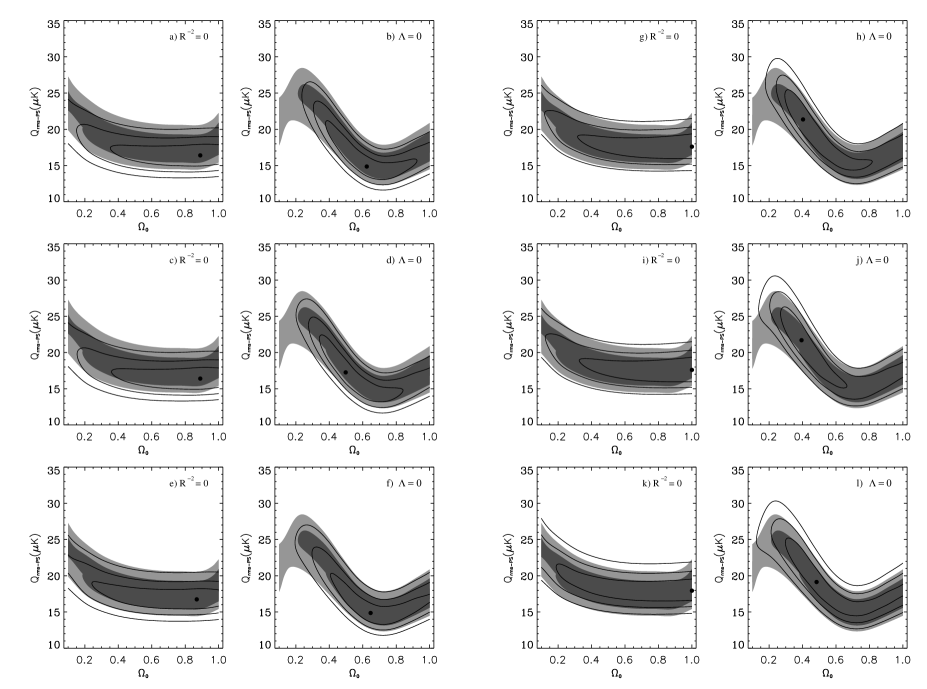
Figure 6: Confidence contours and maxima of the marginalized two-dimensional $(Q_{\rm rms-PS},\Omega_{0})$ posterior probability density distribution functions. Panels $a)$, $c)$, & $e)$ in the first column and $g)$, $i)$, & $k)$ in the third column show the flat-$\Lambda$ model while panels $b)$, $d)$, & $f)$ in the second column and $h)$, $j)$, & $l)$ in the fourth column show the open model. Shaded regions show the two-dimensional posterior probability density distribution function confidence limits for the DMR data (see Fig. 2 caption for details). Lines show the two-dimensional posterior probability density distribution function 1, 2, and 3 $\sigma$ confidence limits derived from the various combination data sets considered. Solid circles show the maxima of the two-dimensional posterior distributions. Lines in panels $a)-f)$ in the two left hand columns use the DMR galactic frame data with quadrupole included and corrected for faint high-latitude galactic emission while lines in panels $g)-l)$ in the two right hand columns use the DMR ecliptic frame data with quadrupole excluded and no other galactic emission correction (G98). Panels in the top row are from an analysis of the DMR and all smaller-angular-scale data, those in the middle row are from an analysis of all but the SuZIE data, and those in the bottom row are from an analysis of the DMR, SP94Ka, Python I–III, MAX 4 ID, MAX 5 HR, and OVRO data sets.

The central two columns of Fig. 3 show the one-dimensional marginalized posterior distribution functions for $\Omega_{B}h^{2}$. Independent of the data set combination considered low values of $\Omega_{B}h^{2}$ are favored, with $\Omega_{B}h^{2}\simeq$ 0.005 (0.007–0.008) favored in the open (flat-$\Lambda$) model. These results are statistically much more significant than, but quite consistent with, those shown in Fig. 6 of R99b.

The last two columns of Fig. 3 show the one-dimensional marginalized posterior distribution functions for $t_{0}$. Independent of the data set combination considered the flat-$\Lambda$ case favors an old universe with $t_{0}\simeq$ 18–20 Gyr (fifth column of Fig. 3), while the open model favors a young universe with $t_{0}\simeq$ 10–12 Gyr (sixth column of Fig. 3). These open model results are very consistent with those shown in Fig. 7 of R99b, while R99b found that flat-$\Lambda$ models favored a young universe with $t_{0}\simeq$ 10–12 Gyr, at odds with what we find here.

More precisely, the one-dimensional distributions for the “most reliable” data in Fig. 3 (the bottom row) indicates that an open (flat-$\Lambda$) model with $\Omega_{0}$ = 0.42 (1.0), or $\Omega_{B}h^{2}$ = 0.005 (0.008), or $t_{0}$ = 10 (18) Gyr is favored, among the models considered. At 2 $\sigma$ confidence the data formally rule out only small regions of parameter space: the data require $\Omega_{0}$ $>0.18$ ($\Omega_{0}$ $>0.10$), or $\Omega_{B}h^{2}$ $<0.027$ ($\Omega_{B}h^{2}$ $<0.026$), or $t_{0}$ $<19$ Gyr ($t_{0}$ $>11$ Gyr) for the open (flat-$\Lambda$) model at 2 $\sigma$.

While the statistical significance of the constraints on cosmological parameters from these combinations of smaller-angular-scale CMB anisotropy data is not high, there are a couple of puzzling issues. The lower $\Omega_{0}\simeq 0.4$ favored in the open case is more easily reconciled with most other estimates of $\Omega_{0}$ than is the higher value of $\Omega_{0}=1$ favored by the CMB anisotropy data in the flat-$\Lambda$ model (see, e.g., Peebles & Ratra 2002). We emphasize however that more recent CMB anisotropy data favor the flat-$\Lambda$ model with low $\Omega_{0}$ (see, e.g., Netterfield et al. 2002; Pryke et al. 2002; Stompor et al. 2001; Scott et al. 2002; Mason et al. 2002). The low values of $\Omega_{B}h^{2}$ favored by the data considered here are also somewhat at odds with the higher values favored by more recent CMB anisotropy data (see, e.g., Netterfield et al. 2002; Pryke et al. 2002; Stompor et al. 2001) and those favored by standard nucleosynthesis theory and the observed deuterium abundances (Burles, Nollett, & Turner 2001); they are, however, more consistent with the lower $\Omega_{B}h^{2}$ value from standard nucleosynthesis theory and the observed helium and lithium abundances (Cyburt, Fields, & Olive 2001). The ages of an open and a flat-$\Lambda$ universe determined from the smaller-angular-scale CMB data used in this paper lie at the opposite ends of the 2 $\sigma$ range of estimates based on the ages of the oldest stars: 11 Gyr $\;{}_{\sim}^{<}\;t_{0}\;{}_{\sim}^{<}\;$ 17 Gyr (see, e.g., Carretta et al. 2000; Krauss & Chaboyer 2001). Given that the CMB anisotropy data considered here are not the most recent, and that the statistical significance of the puzzling aspects of the derived results are not high, perhaps similar analyses of more recent and future data will show that these puzzles are only apparent.

Figure 4 shows the one-dimensional posterior distribution functions for $Q_{\rm rms-PS}$, derived by marginalizing the four-dimensional ones over the other three parameters. The three different combinations of smaller-angular-scale data sets considered here result in fairly tight constraints on $Q_{\rm rms-PS}$. At 2 $\sigma$ confidence they are consistent with the DMR results for both the open and flat-$\Lambda$ models.

The peak values of the one-dimensional posterior distributions shown in Figs. 3 and 4 are listed in the figure captions for the case when the four-dimensional posterior distributions are normalized such that $L(Q_{\rm rms-PS}\ =\ 0\ \mu{\rm K})\ =\ 1$. With this normalization, marginalizing over the remaining parameter the fully marginalized posterior distributions are, for the open (flat-$\Lambda$) models: $1\times 10^{272}(4\times 10^{271})$ for all the data; $1\times 10^{272}(2\times 10^{271})$ for all the data excluding SuZIE; and, $1\times 10^{202}(8\times 10^{201})$ for the SP94Ka, Python I–III, MAX 4 ID, MAX 5 HR, and OVRO combination. These numerical values are consistent with the indications from the first two columns of Fig. 3 that the data mildly favor the open model over the flat-$\Lambda$ one (since the $\Omega_{0}=1$ models at the right edges of pairs of panels in each row of Fig. 3 are identical).

6 Including the DMR Data: Results and Discussion

As mentioned above, cosmological parameter constraints derived from the DMR data are somewhat sensitive to whether the measured DMR quadrupole moment is included in or excluded from the analysis. To account for this source of uncertainty we consider the two most extreme (in terms of $Q_{\rm rms-PS}$ normalization) DMR data combinations (G98; Stompor 1997): (i) the galactic frame data including the quadrupole moment and correcting for faint high-latitude galactic emission; and (ii) the ecliptic frame data with the quadrupole moment excluded and no other galactic emission correction. Since we consider three different combinations of smaller-angular-scale data, combining these two DMR data sets with the smaller-angular-scale data results in the six different combinations of CMB anisotropy data we consider in this section.

When the smaller-angular-scale data of $\S$ 5 are augmented with the DMR data, the four-dimensional posterior probability density distribution function $L(Q_{\rm rms-PS},\Omega_{0},\Omega_{B}h^{2},t_{0})$ becomes much more peaked in the $t_{0}$ direction (in addition to being peaked in the $Q_{\rm rms-PS}$ direction) but is still somewhat flat in the other two directions. As discussed in $\S$ 5, marginalizing over $Q_{\rm rms-PS}$ and one other parameter results in two-dimensional posterior probability functions which are more peaked. Examples are shown in Fig. 5. Comparing to the corresponding plots (Fig. 1) based on just the smaller-angular-scale data, one sees that the inclusion of the DMR data significantly tightens the constraints on cosmological parameters.

For example, Fig. 5 shows that, independent of data set combination considered, flat-$\Lambda$ models with parameter values near $\Omega_{0}\sim 0.1$, $\Omega_{B}h^{2}\sim 0.03$, and $t_{0}\sim 20$ Gyr, and open models with $\Omega_{0}\;{}_{\sim}^{<}\;0.2$, are both formally ruled out at $\sim 3$ $\sigma$ confidence.

Figure 6 shows the contours of the two-dimensional posterior distribution for $Q_{\rm rms-PS}$ and $\Omega_{0}$, derived by marginalizing the four-dimensional distribution over $\Omega_{B}h^{2}$ and $t_{0}$. These should be compared to the corresponding contours for just the smaller-angular-scale data which are shown in Fig. 2. The addition of the DMR data significantly tightens the constraints.

Figure 7 shows the one-dimensional posterior distribution functions for $\Omega_{0}$, derived by marginalizing the four-dimensional ones over the other three parameters. For the flat-$\Lambda$ model, using the galactic frame DMR data with quadrupole included and corrected for faint high-latitude galactic emission, in conjunction with the smaller-angular-scale data, results in $\Omega_{0}\simeq 0.9$ being favored (first column of Fig. 7), while the ecliptic frame DMR data with quadrupole excluded and no further correction for foreground contamination results in $\Omega_{0}=1$ being favored (third column of Fig. 7). In the open case, the galactic-frame quadrupole-included DMR data, in conjunction with the smaller-angular-scale data, favor $\Omega_{0}\sim 0.5-0.6$ (second column of Fig. 7), while the ecliptic-frame quadrupole-excluded DMR data set combination favor $\Omega_{0}\simeq 0.4$ (fourth column of Fig. 7). Perhaps the most reliable constraints follow from panels $k$ and $l$ of Fig. 7, which are derived from the ecliptic frame DMR data with quadrupole excluded and no further correction for foreground emission, used in conjunction with the smaller-angular-scale data from the SP94Ka, Python I–III, MAX 4 ID, MAX 5 HR, and OVRO experiments. In this case, the favored value of $\Omega_{0}$ is 1.0 (0.43) with $\Omega>0.17$ $(0.29<\Omega_{0}<0.93)$ required at 2 $\sigma$ for the flat-$\Lambda$ (open) models. Since the two $\Omega_{0}=1$ models at the right hand edges of each pair of plots are identical, when the flat-$\Lambda$ and open model posterior probability distribution functions are renormalized to make this $\Omega_{0}=1$ model have the same probability in both cases, the probability for $\Omega_{0}=0.3$ (which is close to what is observed, see, e.g., Peebles & Ratra 2002) is about 50% higher in the open case than in the flat-$\Lambda$ case. While not highly statistically significant it is still interesting that the open “foil” provides a better fit to this data than does the “favored” flat-$\Lambda$ model. It should also be noted that this conclusion also follows from the smaller-angular-scale data alone: see the first two columns of Fig. 3. It is puzzling why these results are not more consistent with those from less exact analysis of more recent CMB anisotropy data, which find that the low-density flat-$\Lambda$ model is favored over the low-density open case (see, e.g., Netterfield et al. 2002; Pryke et al. 2002; Stompor et al. 2001). Perhaps the data used in this paper has undetected systematic errors, or perhaps it is the more recent data which has these (we note that some of the more recent data analyses require use of “prior” assumptions before they hone in on the “favored” flat-$\Lambda$ model). It appears that an analysis of more data than considered here will be needed to resolve this issue.

Figure 8 shows the one-dimensional marginalized posterior distribution functions for $\Omega_{B}h^{2}$. For both the flat-$\Lambda$ and open models, and for all combined data sets considered, a low $\Omega_{B}h^{2}\simeq 0.005-0.009$ is favored. For the most reliable data combination, the DMR ecliptic frame data with quadrupole excluded and no other correction for foreground emission, in conjunction with the SP94Ka, Python I-III, MAX 4 ID, MAX 5 HR, and OVRO data sets (panels $k$ and $l$ of Fig. 8), $\Omega_{B}h^{2}=0.007$ is favored in both the flat-$\Lambda$ and open cases, with $\Omega_{B}h^{2}<0.026$ ($\Omega_{B}h^{2}<0.027$) required at 2 $\sigma$ for the flat-$\Lambda$ (open) models. These values are somewhat lower than what are favored by less exact analyses of more recent CMB anisotropy data (see, e.g., Netterfield et al. 2002; Pryke et al. 2002; Stompor et al. 2001) and those derived from standard nucleosynthesis theory and the observed deuterium abundances (Burles, Nollett, & Turner 2001); they are, however, more consistent with the lower $\Omega_{B}h^{2}$ value from standard nucleosynthesis theory and the observed helium and lithium abundances (Cyburt, Fields, & Olive 2001). These values are consistent with those derived using only the smaller-angular-scale data (see the central two columns of Fig. 3).

Figure 9 shows the one-dimensional marginalized posterior distribution functions for $t_{0}$. The flat-$\Lambda$ model favors $t_{0}\sim 12-15$ Gyr, while the open model favors $t_{0}\sim 12-14$ Gyr. The open case is very consistent with the results from the smaller-angular-scale anisotropy data alone (see the last column of Fig. 3), however, the smaller-angular-scale data alone favors $t_{0}\sim 18-20$ Gyr for the flat-$\Lambda$ model (see the second last column of Fig. 3), larger than what is favored when the DMR data is included in the mix. For the most reliable data combination, the DMR ecliptic frame data with quadrupole excluded and no other correction for foreground emission, in conjunction with the SP94Ka, Python I-III, MAX 4 ID, MAX 5 HR, and OVRO data (panels $k$ and $l$ of Fig. 9), $t_{0}=13$ Gyr is favored, with $t_{0}<19$ Gyr required at 2 $\sigma$ for both the open and flat-$\Lambda$ cases. These values are in excellent accord with estimates for the age of the universe from the ages of the oldest stars (see, e.g., Carretta et al. 2000; Krauss & Chaboyer 2001).

Figure 10 shows the one-dimensional posterior distribution functions for $Q_{\rm rms-PS}$, derived by marginalizing the four-dimensional ones over the other three parameters. The CMB anisotropy data lead to tight constraints on $Q_{\rm rms-PS}$.

The peak values of the one-dimensional posterior distributions shown in Figures 7–10 are listed in the figure captions for the case when the four-dimensional posterior distributions are normalized such that $L(Q_{\rm rms-PS}\ =\ 0\ \mu{\rm K})\ =\ 1$. With this normalization, marginalizing over the remaining parameter the fully marginalized posterior distributions are, for the flat-$\Lambda$ (open) models: $3\times 10^{435}(7\times 10^{435})$ for the galactic-frame quadrupole-included faint-high-latitude-foreground-corrected DMR data in conjunction with the smaller-angular-scale data; $1\times 10^{435}(5\times 10^{435})$ for this data less the SuZIE data; $6\times 10^{365}(7\times 10^{365})$ for this DMR data and the SP94Ka, Python I-III, MAX 4 ID, MAX 5 HR, and OVRO smaller-angular-scale data; $3\times 10^{440}(1\times 10^{441})$ for the ecliptic-frame quadrupole-excluded, and no other correction for foreground emission, DMR data in conjunction with the smaller-angular-scale data; $2\times 10^{440}(1\times 10^{441})$ for this data less the SuZIE data; and, $1\times 10^{371}(2\times 10^{371})$ for this DMR data and the SP94Ka, Python I-III, MAX 4 ID, MAX 5 HR, and OVRO smaller-angular-scale data. These numerical values are consistent with the indications from Fig. 7 that the open case is mildly favored over the flat-$\Lambda$ model.

7 Conclusion

We have derived constraints on cosmological model parameters in the open and flat-$\Lambda$ CDM models, from joint analyses of combinations of the DMR, SP94, Python I–III, ARGO, MAX 4+5, White Dish, OVRO, and SuZIE CMB anisotropy data sets. The constraints derived here are not of very high statistical significance.

The data considered here mildly favor the open case over the flat-$\Lambda$ model, although they do not rule out the currently favored flat-$\Lambda$ model with $\Omega_{0}\sim 0.3$. The favored value of $\Omega_{0}$ in the open ($\Omega_{0}\sim 0.4-0.6$) and flat-$\Lambda$ ($\Omega_{0}\sim 0.9-1$) models are somewhat dependent on whether the DMR quadrupole moment is included in or excluded from the analysis. Resolving this issue will likely require analyses that use new higher quality large angular scale CMB anisotropy and foreground emission data.

Constraints on $\Omega_{B}h^{2}$ and $t_{0}$ are only weakly dependent on the data set combination considered. The data considered here favors lower $\Omega_{B}h^{2}\sim 0.005-0.009$, or younger, $t_{0}\sim 12-15$ Gyr, universes.

Some of the constraints derived here are mildly inconsistent with those derived elsewhere, but gratifyingly not so at high statistical significance. Tighter and more robust constraints on cosmological parameters will require a models-based joint analysis of a larger collection of CMB anisotropy data sets.

We acknowledge valuable assistance from R. Stompor. This work was partially carried out at the California Institute of Technology IPAC and JPL, under a contract with NASA. PM, BR, and TS acknowledge support from NSF CAREER grant AST-9875031. NS acknowledges support from the Alexander von Humboldt Foundation and Japanese Grant-in-Aid for Science Research Fund No. 14540290.

Figure 1: Confidence contours and maxima of the two-dimensional posterior probability density distribution functions, as a function of the two parameters on the axes of each panel (derived by marginalizing the four-dimensional posterior distributions over the other two parameters). Dashed lines (crosses) show the contours (maxima) of the open case and solid lines (solid circles) show those of the flat-$\Lambda$ model. Contours of 0.25, 0.5, 1, 2, and 3 $\sigma$ confidence are shown (some contours are not labelled). Panels $a)-c)$ in the left column show the $(\Omega_{B}h^{2},\ \Omega_{0})$ plane, while panels $d)-f)$ in the right column show the $(t_{0},\ \Omega_{0})$ plane. Panels $a)$ & $d)$ in the top row are from an analysis of all the small scale data. Panels $b)$ & $e)$ in the middle row are from an analysis of all but the SuZIE small scale data. Panels $c)$ & $f)$ in the bottom row are from an analysis of the SP94Ka, Python I–III, MAX 4 ID, MAX 5 HR, and OVRO data sets.

Figure 3: One-dimensional posterior probability density distribution functions for $\Omega_{0}$ (two left most columns), for $\Omega_{B}h^{2}$, (two central columns), and for $t_{0}$ (two right most columns), derived by marginalizing the four-dimensional ones over the other three parameters, in the open and flat-$\Lambda$ models. These have been renormalized to unity at the peaks. Dotted lines show the formal 1, 2, and 3 $\sigma$ confidence limits derived from these one-dimensional posterior distributions. Panels $a)$, $c)$, & $e)$ in the first column, $g)$, $i)$, & $k)$ in the third column, and $m)$, $o)$, & $q)$ in the fifth column show the flat-$\Lambda$ model and panels $b)$, $d)$, & $f)$ in the second column, $h)$, $j)$, & $l)$ in the fourth column, and $n)$, $p)$, and $r)$ in the sixth column show the open model. Panels in the top row are from an analysis of all the small scale data, those in the middle row are from an analysis of all but the SuZIE small scale data, and those in the bottom row are from an analysis of the SP94Ka, Python I-III, MAX 4 ID, MAX 5 HR, and OVRO data sets. When the four-dimensional posterior distributions are normalized such that $L(Q_{\rm rms-PS}\ =\ 0\ \mu{\rm K})\ =\ 1$, the peak values of the one-dimensional distributions shown in panels $a)-f)$ are $6\times 10^{271}$, $2\times 10^{272}$, $3\times 10^{271}$, $2\times 10^{272}$, $1\times 10^{202}$, and $2\times 10^{202}$, respectively; in panels $g)-l)$ are $3\times 10^{273}$, $7\times 10^{273}$, $1\times 10^{273}$, $6\times 10^{273}$, $5\times 10^{203}$, and $7\times 10^{203}$, respectively; and in panels $m)-r)$ are $6\times 10^{270}$, $1\times 10^{271}$, $3\times 10^{270}$, $1\times 10^{271}$, $9\times 10^{200}$, and $1\times 10^{201}$, respectively.

Figure 4: One-dimensional posterior probability density distribution functions for $Q_{\rm rms-PS}$, derived by marginalizing the four-dimensional ones over the other three parameters, in the open and flat-$\Lambda$ models. Conventions are as described in the caption of Fig. 3. Solid vertical lines show the $\pm 1$, $\pm 2$, and $\pm 3$ $\sigma$ confidence limits derived by projecting the corresponding small-scale data four-dimensional posterior distributions. Also shown are the 2 $\sigma$ DMR (marginalized and projected) confidence limits; these are a composite of those from the two extreme DMR data sets (see caption of Fig. 2). When the four-dimensional posterior distributions are normalized such that $L(Q_{\rm rms-PS}\ =\ 0\ \mu{\rm K})\ =\ 1$, the peak values of the one-dimensional distributions shown in panels $a)-f)$ are $9\times 10^{270}$, $1\times 10^{271}$, $4\times 10^{270}$, $8\times 10^{270}$, $1\times 10^{201}$, and $1\times 10^{201}$, respectively.

Figure 5: Confidence contours and maxima of the two-dimensional posterior probability density distribution functions, as a function of the two parameters on the axes of each panel (derived by marginalizing the four-dimensional posterior distributions over the other two parameters). Dashed lines (crosses) show the contours (maxima) of the open case and solid lines (solid circles) show those of the flat-$\Lambda$ model. Contours of 0.25, 0.5, 1, 2, and 3 $\sigma$ confidence are shown (some contours are not labelled). Panels $a)-c)$ in the first column and panels $g)-i)$ in the third column show the $(\Omega_{B}h^{2},\ \Omega_{0})$ plane, while panels $d)-f)$ in the second column and panels $j)-l)$ in the fourth show the $(t_{0},\ \Omega_{0})$ plane. Panels $a)-f)$ in the two left hand columns use the DMR galactic frame data with quadrupole included and corrected for faint high-latitude galactic emission while panels $g)-l)$ in the two right hand columns use the DMR ecliptic frame data with quadrupole excluded and no other galactic emission correction (G98). Panels in the top row are from an analysis of the DMR and all smaller-angular-scale data, those in the middle row are from an analysis of all but the SuZIE data, and those in the bottom row are from an analysis of the DMR, SP94Ka, Python I–III, MAX 4 ID, MAX 5 HR, and OVRO data sets.

Figure 7: One-dimensional posterior probability density distribution functions for $\Omega_{0}$, derived by marginalizing the four-dimensional ones over the other three parameters, in the open and flat-$\Lambda$ models. These have been renormalized to unity at the peaks. Dotted lines show the formal 1, 2, and 3 $\sigma$ confidence limits derived from these one-dimensional posterior distributions. Panels $a)$, $c)$, & $e)$ in the first column, and $g)$, $i)$, & $k)$ in the third column show the flat-$\Lambda$ model while panels $b)$, $d)$, & $f)$ in the second column, and $h)$, $j)$, & $l)$ in the fourth column show the open model. Panels $a)-f)$ in the two left hand columns use the DMR galactic frame data with quadrupole included and corrected for faint high-latitude galactic emission while lines in panels $g)-l)$ in the two right hand columns use the DMR ecliptic frame data with quadrupole excluded and no other galactic emission correction (G98). Panels in the top row are from an analysis of the DMR and all smaller-angular-scale data, those in the middle row are from an analysis of all but the SuZIE data, and those in the bottom row are from an analysis of the DMR, SP94Ka, Python I–III, MAX 4 ID, MAX 5 HR, and OVRO data sets. When the four-dimensional posterior distributions are normalized such that $L(Q_{\rm rms-PS}\ =\ 0\ \mu{\rm K})\ =\ 1$, the peak values of the one-dimensional distributions shown in panels $a)-l)$ are $5\times 10^{435}$, $1\times 10^{436}$, $2\times 10^{435}$, $1\times 10^{436}$, $1\times 10^{366}$, $1\times 10^{366}$, $6\times 10^{440}$, $4\times 10^{441}$, $3\times 10^{440}$, $6\times 10^{441}$, $2\times 10^{371}$, and $4\times 10^{371}$, respectively.

Figure 8: One-dimensional posterior probability density distribution functions for $\Omega_{B}h^{2}$, derived by marginalizing the four-dimensional ones over the other three parameters, in the open and flat-$\Lambda$ models. Conventions are as described in the caption of Fig. 7. When the four-dimensional posterior distributions are normalized such that $L(Q_{\rm rms-PS}\ =\ 0\ \mu{\rm K})\ =\ 1$, the peak values of the one-dimensional distributions shown in panels $a)-l)$ are $2\times 10^{437}$, $6\times 10^{437}$, $1\times 10^{437}$, $3\times 10^{437}$, $4\times 10^{367}$, $4\times 10^{367}$, $3\times 10^{442}$, $1\times 10^{443}$, $2\times 10^{442}$, $9\times 10^{442}$, $8\times 10^{372}$, and $1\times 10^{373}$, respectively.

Figure 9: One-dimensional posterior probability density distribution functions for $t_{0}$, derived by marginalizing the four-dimensional ones over the other three parameters, in the open and flat-$\Lambda$ models. Conventions are as described in the caption of Fig. 7. When the four-dimensional posterior distributions are normalized such that $L(Q_{\rm rms-PS}\ =\ 0\ \mu{\rm K})\ =\ 1$, the peak values of the one-dimensional distributions shown in panels $a)-l)$ are $4\times 10^{434}$, $1\times 10^{435}$, $2\times 10^{434}$, $8\times 10^{434}$, $9\times 10^{364}$, $9\times 10^{364}$, $6\times 10^{439}$, $3\times 10^{440}$, $3\times 10^{439}$, $2\times 10^{440}$, $2\times 10^{370}$, and $3\times 10^{370}$, respectively.

Figure 10: One-dimensional posterior probability density distribution functions for $Q_{\rm rms-PS}$, derived by marginalizing the four-dimensional ones over the other three parameters, in the open and flat-$\Lambda$ models. Conventions are as described in the caption of Fig. 7. Also shown here as solid vertical lines are $\pm 1$, $\pm 2$, and $\pm 3$ $\sigma$ confidence limits derived by projecting the corresponding four-dimensional posterior distributions, as well as the 2 $\sigma$ DMR (marginalized and projected) confidence limits which are a composite of those from the two extreme DMR data sets (see caption of Fig. 2). When the four-dimensional posterior distributions are normalized such that $L(Q_{\rm rms-PS}\ =\ 0\ \mu{\rm K})\ =\ 1$, the peak values of the one-dimensional distributions shown in panels $a)-l)$ are $8\times 10^{434}$, $1\times 10^{435}$, $4\times 10^{434}$, $1\times 10^{435}$, $2\times 10^{365}$, $2\times 10^{365}$, $1\times 10^{440}$, $2\times 10^{440}$, $5\times 10^{439}$, $2\times 10^{440}$, $4\times 10^{370}$, and $3\times 10^{370}$, respectively.

References

- Bartelmann et al. (2002) Bartelmann, M., Perrotta, F., & Baccigalupi, C. 2002, astro-ph/0206507
- Bennett et al. (1996) Bennett, C. L., et al. 1996, ApJ, 464, L1
- Brax, Martin, & Riazuelo (2000) Brax, P., Martin, J., & Riazuelo, A. 2000, Phys. Rev. D, 62, 103505
- Burles et al. (2001) Burles, S., Nollett, K. M., & Turner, M. S. 2001, ApJ, 552, L1
- Carretta et al. (2000) Carretta, E., Gratton, R. G., Clementini, G., & Pecci, F. F. 2000, ApJ, 533, 215
- Carroll (2001) Carroll, S.M. 2001, Living Rev. Relativity, 4, 1
- Chen & Ratra (2002) Chen, G., & Ratra, B. 2002, ApJ, in press, astro-ph/0207051
- Church et al. (1997) Church, S. E., Ganga, K. M., Ade, P. A. R., Holzapfel, W. L., Mauskopf, P. D., Wilbanks, T. M., & Lange, A. E. 1997, ApJ, 484, 523
- Coble et al. (2001) Coble, K., Dodelson, S., Dragovan, M., Ganga, K., Knox, L., Kovac, J., Ratra, B., & Souradeep, T. 2001, astro-ph/0112506
- Cyburt et al. (2001) Cyburt, R. H., Fields, B. D., & Olive, K. A. 2001, New Astron., 6, 215.
- Dave et al. (2002) Dave, R., Caldwell, R. R., & Steinhardt, P. J. 2002, astro-ph/0206372
- de Bernardis et al. (1994) de Bernardis, P., et al. 1994, ApJ, 422, L33
- de Oliveira-Costa et al. (1998) de Oliveira-Costa, A. Tegmark, M., Page, L. A., & Boughn, S. P. 1998, ApJ, 509, L9
- Efstathiou et al. (1990) Efstathiou, G., Sutherland, W. J., & Maddox, S. J. 1990, Nature, 348, 705
- Fischler et al. (1985) Fischler, W., Ratra, B., & Susskind, L. 1985, Nucl. Phys. B, 259, 730.
- Ganga et al. (1997b) Ganga, K., Ratra, B., Church, S. E., Sugiyama, N., Ade, P. A. R., Holzapfel, W. L., Mauskopf, P.D., & Lange, A. E. 1997b, ApJ, 484, 517
- Ganga et al. (1997a) Ganga, K., Ratra, B., Gundersen, J. O., & Sugiyama, N. 1997a, ApJ, 484, 7 (GRGS)
- Ganga et al. (1998) Ganga, K., Ratra, B., Lim, M. A., Sugiyama, N., & Tanaka, S. T. 1998, ApJS, 114, 165
- Gorski et al. (1998) Górski, K. M., Ratra, B., Stompor, R., Sugiyama, N., & Banday, A. J. 1998, ApJS, 114, 1
- Gott (1982) Gott, J.R. 1982, Nature, 295, 304
- Gundersen et al. (1995) Gundersen, J. O., et al. 1995, ApJ, 443, L57
- Hamilton & Ganga (2001) Hamilton, J.-Ch., & Ganga, K. 2001, A&A, 368, 760
- Kogut et al. (1996) Kogut, A., Banday, A. J., Bennet, C. L., Górski, K. M., Hinshaw, G., Smoot, G. F. & Wright, E. L. 1996, ApJ, 464, L5
- Komatsu et al. (2002) Komatsu, E., Wandelt, B. D., Spergel, D. N., Banday, A. J., & Górski, K. M. 2002, ApJ, 566, 19
- Krauss & Chaboyer (2001) Krauss, L. M., & Chaboyer, B. 2001, astro-ph/0111597
- Leitch et al. (2000) Leitch, E. M., Readhead, A. C. S., Pearson, T. J., Myers, S. T., Gulkis, S., & Lawrence C. R. 2000, ApJ, 532, 37
- Lewis & Bridle (2002) Lewis, A., & Bridle, S. 2002, astro-ph/0205436
- Lim et al. (1996) Lim, M. A., et al. 1996, ApJ, 469, L69
- Mason et al. (2002) Mason, B. S., et al. 2002, astro-ph/0205384
- Miller et al. (2002a) Miller, A. D., et al. 2002a, ApJS, 140, 115
- Miller et al. (2002b) Miller, C. J., Nichol, R. C., Genovese, C., & Wasserman, L. 2002b, ApJ, 565, L67
- Mukherjee et al. (2002a) Mukherjee, P., Dennison, B., Ratra, B., Simonetti, J. H., Ganga, K., & Hamilton, J.-Ch. 2002a, ApJ (in press), astro-ph/0110457
- Mukherjee et al. (2000) Mukherjee, P., Hobson, M. P., & Lasenby, A. N. 2000, MNRAS, 318, 1157
- Mukherjee et al. (2002b) Mukherjee, P., Souradeep, T., Ratra, B., Sugiyama, N., & Górski, K. M. 2002b, astro-ph/0208216
- Munshi & Wang (2002) Munshi, D., & Wang, Y. 2002, astro-ph/0206483
- Netterfield et al. (2002) Netterfield, C. B., et al. 2002, ApJ, 571, 604
- Park et al. (2001) Park, C.-G., Park, C., Ratra, B., & Tegmark, M. 2001, ApJ, 556, 582
- Peebles (1984) Peebles, P. J. E. 1984, ApJ, 284, 439
- Peebles & Ratra (1988) Peebles, P. J. E., & Ratra, B. 1988, ApJ, 325, L17
- Peebles & Ratra (2002) Peebles, P. J. E., & Ratra, B. 2002, astro-ph/0207347
- Platt et al. (1997) Platt, S. R., Kovac, J., Dragovan, M., Peterson, J. B., & Ruhl, J. E. 1997, ApJ, 475, L1
- Podariu et al. (2002) Podariu, S., Daly, R. A., Mory, M. P., & Ratra, B. 2002, astro-ph/0207096
- Podariu et al. (2001) Podariu, S., Souradeep, T., Gott, J. R., Ratra, B., & Vogeley, M. S. 2001, ApJ, 559, 9
- Polenta et al. (2002) Polenta, G., et al. 2002, ApJ, 572, L27
- Pryke et al (2002) Pryke, C., Halverson, N. W., Leitch, E. M., Kovac, J., Carlstrom, J. E., Holzapfel, W. L., & Dragovan, M. 2002, ApJ, 568, 46
- Ratra (1985) Ratra, B. 1985, Phys. Rev. D, 31, 1931
- Ratra et al. (1999a) Ratra, B., Ganga, K., Stompor, R., Sugiyama, N., de Bernardis, P., & Górski, K. M. 1999a, ApJ, 510, 11 (R99a)
- Ratra et al. (1998) Ratra, B., Ganga, K., Sugiyama, N., Tucker, G. S., Griffin, G. S., Nguyên, H. T., & Peterson, J. B. 1998, ApJ, 505, 8
- Ratra & Peebles (1995) Ratra, B., & Peebles, P. J. E. 1995, Phys. Rev. D, 52, 1837
- Ratra & Quillen (1992) Ratra, B., & Quillen, A. 1992, MNRAS, 259, 738
- Ratra et al. (1999b) Ratra, B., Stompor, R., Ganga, K., Rocha, G., Sugiyama, N., & Górski, K. M. 1999b, ApJ, 517, 549 (R99b)
- Ratra et al. (1997) Ratra, B., Sugiyama, N., Banday, A. J., & Górski, K. M. 1997, ApJ, 481, 22
- Rocha et al. (1999) Rocha, G., Stompor, R., Ganga, K., Ratra, B., Platt, S. R., Sugiyama, N., & Górski, K. M. 1999, ApJ, 525, 1
- Sahni & Starobinsky (2000) Sahni, V., & Starobinsky, A. 2000, Int. J. Mod. Phys. D, 9, 373
- Santos et al. (2002) Santos, M. G., et al. 2002, Phys. Rev. Lett., 88, 241302
- Scott et al. (2002) Scott, P. F., et al. 2002, astro-ph/0205380
- Shandarin et al. (2002) Shandarin, S. F., Feldman, H. A., Xu, Y., & Tegmark, M. 2002, ApJS, 141, 1
- Sievers et al. (2002) Sievers, J. L., et al. 2002, astro-ph/0205387
- Steinhardt (1999) Steinhardt, P.J. 1999, in Proceedings of the Pritzker Symposium on the Status of Inflationary Cosmology, in press
- Stompor (1997) Stompor, R. 1997, in Microwave Background Anisotropies, ed. F. R. Bouchet, R. Gispert, B. Guiderdoni, & J. Tran Thanh Van (Gif-sur-Yvette: Editions Frontieres), 91
- Stompor et al. (2001) Stompor, R., et al. 2001, ApJ, 561, L7
- Stompor et al. (1995) Stompor, R., Górski, K. M., & Banday, A. J. 1995, MNRAS, 277, 1225
- Tucker et al. (1993) Tucker, G. S., Griffin, G. S., Nguyên, H. T., & Peterson, J. B. 1993, ApJ, 419, L45
- Wang et al. (2002) Wang, X., Tegmark, M., & Zaldarriaga, M. 2002, Phys. Rev. D, 65, 123001
- Wu et al. (2001) Wu, J.-H. P., et al. 2001, Phys. Rev. Lett., 87, 251303