A Study of the Direct-Fitting Method
for Measurement of Galaxy Velocity Dispersions

Abstract

We have measured the central stellar velocity dispersions of 33 nearby spiral and elliptical galaxies, using a straightforward template-fitting algorithm operating in the pixel domain. The spectra, obtained with the Double Spectrograph at Palomar Observatory, cover both the Ca triplet and the Mg Ib region, and we present a comparison of the velocity dispersion measurements from these two spectral regions. Model fits to the Ca triplet region generally yield good results with little sensitivity to the choice of template star. In contrast, the Mg Ib region is more sensitive to template mismatch and to details of the fitting procedure such as the order of a polynomial used to match the continuum shape of the template to the object. As a consequence of the correlation of the [Mg/Fe] ratio with velocity dispersion, it is difficult to obtain a satisfactory model fit to the Mg Ib lines and the surrounding Fe blends simultaneously, particularly for giant elliptical galaxies with large velocity dispersions. We demonstrate that if the metallicities of the galaxy and template star are not well matched, then direct template-fitting results are improved if the Mg Ib lines themselves are excluded from the fit and the velocity dispersion is determined from the surrounding weaker lines.

1 Introduction

The recent discovery of a tight correlation between stellar velocity dispersion and black hole mass (the $M_{\mathrm{\bullet}}-\sigma$ relation; Ferrarese & Merritt, 2000; Gebhardt et al., 2000) has placed new emphasis on the importance of accurate velocity dispersion measurements for the central regions of nearby galaxies. Since black hole mass is approximately proportional to $\sigma^{4}$, even modest errors in $\sigma$ for galaxies with black hole mass measurements can have a substantial impact on the correlation (Tremaine et al., 2002). Use of the predictive power of the $M_{\mathrm{\bullet}}-\sigma$ relation to obtain estimates of the masses of black holes in galaxy nuclei also relies on the accuracy of the velocity dispersion measurements. In view of these issues, it is worthwhile to examine the level of agreement between velocity dispersion measurements obtained with different techniques and from different spectral regions, to determine the methods that are most likely to yield accurate results.

This paper presents an examination of a simple direct template-fitting technique operating in the wavelength domain. Initially, our main goal was to measure velocity dispersions for the sample of nearby galaxies observed with Chandra by Ho et al. (2001), so that estimates of the black hole masses in these galaxies could be derived by applying the $M_{\mathrm{\bullet}}-\sigma$ relation. We were able to observe most of the galaxies from this sample during two observing runs. We also observed some other nearby galaxies for which no previous velocity dispersion measurements were available, a few velocity dispersion “standard” galaxies from McElroy (1995) for comparison, and several low-redshift BL Lac objects for which the results have been reported separately (Barth, Ho, & Sargent, 2002a, b). Here, we present velocity dispersions for 33 nearby galaxies and a comparison of measurements obtained from the Ca triplet and Mg Ib spectral regions. We also discuss some systematic issues relevant to the application of the direct template-fitting method. In particular, we demonstrate that model fits to the Mg Ib spectral region are sensitive to the [Mg/Fe] abundance ratio, and that the results are usually improved if the Mg Ib lines themselves are excluded from the fitting region used to determine the velocity dispersion.

2 Observations and Reductions

The data were obtained during two observing runs with the Double Spectrograph (Oke & Gunn, 1982) at the Palomar Hale 5m telescope, in 2001 June and 2002 January. The red side setup was identical during the two runs. For the blue side, we used a 600 lines mm^-1 grating during the 2001 June run, and a 1200 lines mm^-1 grating during the 2002 January run. The setups and instrumental dispersions are listed in Table 1. Conditions were mediocre during both runs, with typical seeing of 1$\farcs$5–2$\farcs$0 and moderate to thick cloud cover during most of the nights. None of the data were obtained in photometric conditions.

The spectrograph slit was oriented at the parallactic angle, so that the blue and red spectra would cover the same region of the galaxy. This allows a more consistent comparison between the red and blue measurements but with the caveat that our measurements do not generally correspond to any particular symmetry axis of the galaxy. Given the mediocre seeing during our observing runs and the fact that the slit position angle is effectively random relative to the galaxy major axis, we choose to measure only the bulk velocity dispersion in a region centered on the nucleus, rather than performing a detailed study of spatially-resolved kinematics. The high signal-to-noise ratio (S/N) of the spectra obtained from these wide extractions allows us to explore various systematic issues in the measurement procedure.

Bias subtraction and flat-fielding were performed in the usual manner using standard IRAF tasks. Extractions were performed over a width of 3$\farcs$74, which corresponds to 8 pixels on the red CCD and 6 pixels on the blue CCD. This extraction width was chosen so that the blue and red measurements would cover exactly the same spatial region of the galaxy, to facilitate comparison of the results. The spectra were extracted optimally (Horne, 1986) in order to maximize the S/N and remove cosmic-ray hits. We verified that there were no differences in line strength or width between the optimally-weighted spectra and normally-weighted extractions over the same extraction widths. The fractional differences in pixel values between the optimal and normal extractions were typically at the level of $\lesssim 10^{-3}$ for well-exposed spectra, except at pixels affected by cosmic-ray hits. Averaged over all galaxies in the sample, the mean S/N per pixel of the extracted spectra is 107 for the red side data, and 224 and 142 for the blue side data obtained with the 600 and 1200 line gratings, respectively, in the wavelength regions used to determine $\sigma$.

The spectra were then wavelength calibrated and flux calibrated using standard techniques. The deep telluric H₂O absorption features longward of 8900 Å were removed by dividing by the normalized spectrum of a standard star, but this spectral region is not used in any of the analysis discussed below. Finally, a small linear shift was applied to the wavelength scale of each exposure based on the wavelengths of night sky emission lines, and in cases where multiple exposures of the same object were taken, they were averaged together.

3 Measurements

3.1 Method

Our observations cover the Ca triplet at $\lambda\lambda$8498, 8542, 8662 Å and the Mg Ib triplet at $\lambda\lambda$5167, 5173, 5184 Å, as well as blends of Fe lines at 5270 and 5335 Å and other weaker lines in the region surrounding Mg Ib. As discussed by Dressler (1984), the Ca triplet region is ideal for velocity dispersion measurements since it is relatively insensitive to differences in stellar populations.

We performed the measurements of $\sigma$ with a direct template-fitting routine. Direct fitting in the pixel domain is the most straightforward method for measuring velocity dispersions (van der Marel, 1994; Rix et al., 1995). One of its main advantages is that it is simple to mask out unwanted spectral features from the fit and compute $\chi^{2}$ only over an exactly specified wavelength range. This is particularly useful for galaxies having emission lines, or when telluric or interstellar absorption lines are in the wavelength range of interest. Direct fitting has the disadvantage of being more computationally expensive than, for example, cross-correlation (Tonry & Davis, 1979) or Fourier quotient (Simkin, 1974; Sargent et al., 1977) methods, but this is no longer a severe limitation with processor speeds currently available.

To measure $\sigma$, the object and template spectra are rebinned to a wavelength scale that is linear in $x=\ln\lambda$, so that velocity shifts can be performed by linear shifts to the log wavelength scale. The logarithmic bin size is chosen to preserve the total number of pixels in the spectrum. The object spectrum $O(x)$ is transformed to zero redshift by setting $O(x_{\mathrm{rest}})=O(x_{\mathrm{observed}}+\ln[1+z])$, where $z$ is the galaxy’s redshift.

Our measurement technique is very similar to the direct-fitting procedure described by Kelson et al. (2000). For simplicity, we assume a Gaussian profile for the line-of-sight velocity distribution (LOSVD). Then, the model $M(x)$ is computed as

$$M(x)=\left\{\left[T(x)\otimes G(x)\right]+C(x)\right\}\times P(x),$$ (1)

where $T$ is the stellar template spectrum, $G$ is the Gaussian broadening function, $C$ is a featureless continuum, $P$ is a low-order Legendre polynomial, and $\otimes$ denotes convolution. The featureless continuum is a straight line of arbitrary slope that allows the model to match the dilution of the galaxy spectrum. A straight line is sufficient to model the featureless continuum since our fits are performed only over a small wavelength range. The multiplicative polynomial $P$ allows for possible differences in continuum shape or reddening between the object and template without requiring an explicit determination of the reddening. The order of the polynomial is kept low to ensure that it does not affect the widths of individual absorption features; we discuss this issue in more detail below. To determine the goodness of fit we calculate $\chi^{2}$ according to

$$\chi^{2}=\sum_{i}\left(\frac{M_{i}-O_{i}}{\epsilon_{i}}\right)^{2},$$ (2)

where $\epsilon(x)$ is the error spectrum corresponding to the object spectrum $O(x)$, and the calculation is performed over all pixels $i$ in the fitting region. The template spectra are assumed to be noise-free as they have much higher S/N than the galaxy spectra. The fit is optimized by minimizing $\chi^{2}$ using a downhill simplex algorithm (Press et al., 1988). To ensure that the global minimum of $\chi^{2}$ is found, the fit is repeated several times with different search parameters. This method can be generalized to include higher-order moments of the velocity profile (van der Marel, 1994) or a blend of templates of different spectral types (Rix & White, 1992; Rix et al., 1995), but in general we found that good fits to the Ca triplet region could be achieved using the simple model of Gaussian-broadened K-giant spectra, at least over the fairly large spectroscopic aperture employed in this study.

For the pixel errors $\epsilon_{i}$ we used the error spectra returned by the IRAF optimal extraction algorithm, calibrated in the same manner as the galaxy spectra. For well-exposed spectra, these errors were found to be essentially identical to error spectra calculated from the Poisson noise, background noise, and CCD readout noise for a given extraction. The uncertainty on $\sigma$ was calculated by finding how much $\sigma$ must be displaced from its best-fit value, with all other parameters allowed to float freely, in order to increase $\chi^{2}$ by unity relative to its minimum value.

Prior to calculating the uncertainty, the pixel errors $\epsilon_{i}$ were rescaled so as to yield $\tilde{\chi}^{2}=1$ (where $\tilde{\chi}^{2}$ denotes $\chi^{2}$ per degree of freedom). This is conservative in that it increases the size of the error bars on $\sigma$, but in practice it results in only a small increase in the uncertainty estimates. We note that in some cases, particularly for observations with lower than average S/N on the red side, the best fit obtained using the original error spectrum would sometimes yield $\tilde{\chi}^{2}<1$; this suggests that the optimal algorithm in IRAF tends to overestimate the pixel errors by a small amount, $\sim 10-20\%$, at low S/N. When this occurred, the pixel errors were not rescaled. We also performed tests of our fitting routine using equal weighting for all pixels rather than using the error spectrum to calculate $\chi^{2}$. Equal weighting gave results virtually identical to weighting by the pixel errors, with differences of $\leq 1$ km s^-1 in both $\sigma$ and its uncertainty. Thus, measurements obtained by the direct fitting method are not adversely affected if no error spectrum is available.

For each measurement, we used 8 template stars of spectral type G7–K5, with luminosity class III or IV; the stars are listed in Table 2. The uncertainty in $\sigma$ is dominated by template mismatch in many cases, particularly for the blue side data, as the scatter in $\sigma$ values for different templates exceeds the uncertainty in a single fit. To account for this scatter, the final measurement uncertainty given for each galaxy is the sum in quadrature of the fitting uncertainty for the best-fitting template and the standard deviation of the measurements from all 8 template stars.

3.2 Fitting Region

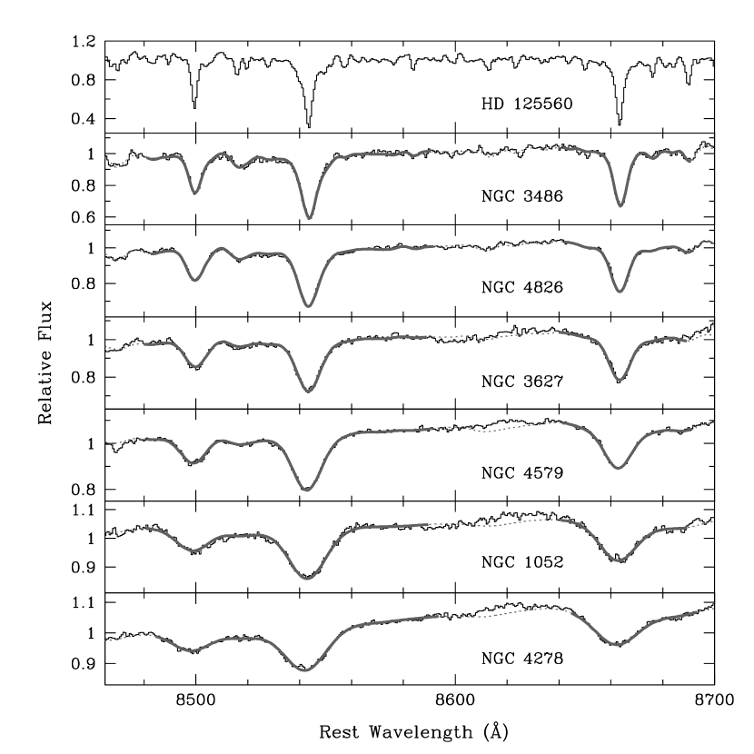
Figure 1: Best fits of broadened stellar templates to the spectra of velocity dispersion standard galaxies from the McElroy (1995) catalog. Regions used to compute $\chi^{2}$ are denoted by a solid thick line, and regions excluded from the fit are indicated by a dotted line.The spectrum of the K3 III star HD 125560 is shown in the top panel.

The fitting regions were chosen to include portions of the spectrum that are sensitive to $\sigma$ but not contaminated by emission lines. On the red side, we used a wavelength region closely surrounding the Ca triplet lines, $8480-8690$ Å. The continuum region $8590-8640$ Å was exluded from the fit as the fits are often poor over this region and there may be [Fe II] emission at 8617 Å in some galaxies (van der Marel, 1994). The continuum regions near the Ca triplet lines have very little sensitivity to $\sigma$ in any case. Figure 1 illustrates the quality of the red side fits over a wide range in $\sigma$. The exclusion of the region $8590-8640$ Å from the fitting region is clearly justified by the poor template match over this wavelength range for NGC 4579, NGC 1052, and NGC 4278.

The blue side data presented additional challenges. Our original intent was to compare the Ca triplet measurements with velocity dispersions measured from the Mg Ib region, and after some trial and error we chose the region $5040-5430$ Å over which reasonable fits could usually be obtained. However, the template spectra often give a very poor match to the Mg Ib lines themselves. While the surrounding region of continuum and weak absorption lines could generally be fit adequately, we found that the fits were usually dramatically improved (in the sense of having a lower value of $\tilde{\chi}^{2}$) by excluding Mg Ib from the fit. The change in $\tilde{\chi}^{2}$ is particularly dramatic for galaxies with high velocity dispersions. We also found it necessary to exclude a small region around 5200 Å, as many galaxies have weak [N I] $\lambda 5200$ Å emission. Even when this line is not clearly visible in the spectra, the fits often reveal a slight excess in the galaxy spectra near 5200 Å relative to the broadened templates. For our final fits, we excluded the range $5150-5210$ Å from the calculation of $\chi^{2}$.

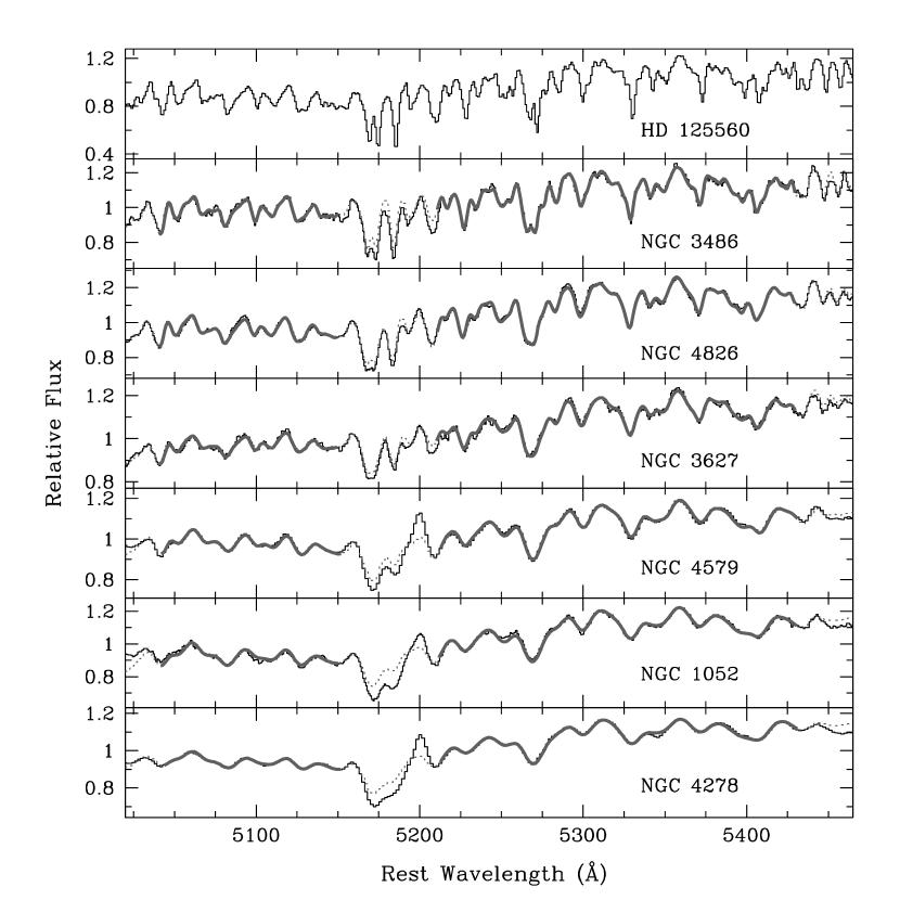
Figure 2: Best fits of broadened stellar templates to the spectra of velocity dispersion standard galaxies from the McElroy (1995) catalog. Regions used to compute $\chi^{2}$ are denoted by a solid thick line. Regions excluded from the fit (the Mg Ib triplet and [N I] $\lambda 5200$) are indicated by a dotted line. The spectrum of the K3 III star HD 125560 is shown in the top panel.

The difficulty of fitting the Mg Ib profile is a consequence of the correlation between Mg Ib line strength and $\sigma$ (Terlevich et al., 1981; Dressler et al., 1987). More specifically, since the ratio [Mg/Fe] in elliptical galaxies is correlated with velocity dispersion (Worthey, Faber, & Gonzalez, 1992; Trager et al., 1998; Kuntschner et al., 2001), galaxies with high $\sigma$ will have stronger Mg Ib absorption relative to the surrounding Fe lines, in comparison with typical nearby giant stars used as velocity templates. Our template stars were chosen based on their spectral type and magnitude, without regard to metallicity, and most have slightly subsolar to slightly above-solar [Fe/H]. The fits shown in Figure 2 demonstrate that with these template stars, it is not possible to achieve a good fit to both the Mg Ib lines and the surrounding region (dominated by Fe blends) for galaxies of high $\sigma$.

As a comparison, we attempted to perform fits using the Mg Ib lines alone, over the range 5150–5190 Å. However, since the Mg lines cover such a small wavelength range, the fits were very poorly constrained even after restricting both the multiplicative polynomial and the featureless continuum to zeroth order (i.e., both flat in $f_{\lambda}$). Consequently, no useful results could be obtained from fitting models only to the Mg Ib lines.

In principle, the [Mg/Fe] mismatch problem could also be alleviated to some extent by observing template stars having a range of super-solar metallicities. However, it would be difficult to find an exact stellar match to the [Mg/Fe] ratio of any given galaxy spectrum, and it would be very time-consuming to observe a grid of template stars with a range in both spectral type and metallicity.

We also note that both the Mg Ib and the Ca triplet lines are intrinsically strong features that are subject to pressure broadening. The widths of these lines in a galaxy spectrum are due to a composite population of stars with a range of surface gravities and therefore a range in intrinsic linewidths. For galaxies with very small velocity dispersions, or for objects such as young super star clusters, it may be preferable to measure velocity dispersions only from regions containing weaker, intrinsically narrow lines, such as the region just redward of Mg Ib (e.g., Ho & Filippenko, 1996).

3.3 Tests of the Measurement Routine

We performed tests to determine whether the measurement routine would yield correct results on a galaxy of known velocity dispersion, including some degree of template mismatch. To perform the tests, we began with a composite template spectrum made by combining a K2 III star, a G2 V star, and a featureless continuum. The weights were chosen so that the total flux in the composite spectrum was 40% K2 III, 40% G2 V, and 20% featureless continuum. The spectrum was then broadened by convolution with Gaussians having $\sigma=50-300$ km s^-1, and its spectral shape was adjusted by multiplication by a 4th-order Legendre polynomial. The polynomial coefficients were restricted so that the continuum flux at any wavelength was modified by $<5\%$. Finally, Poisson noise was added to the broadened spectrum to give S/N = 120 per pixel. The velocity dispersions were measured using the same techniques described above and the same set of template spectra. For the blue side, the simulated data were created using spectra observed with the 1200 line grating.

For both the blue and red sides, the measurement routine is very successful at recovering the correct velocity dispersion over the entire range of $50-300$ km s^-1. In all cases, the measured dispersion is within 6 km s^-1 of the input dispersion. The red side measurements are systematically closer to the input dispersion than the blue side results are, however: the RMS disagreement between the measured and input velocity dispersions is 3.0 km s^-1 for the red side and 4.4 km s^-1 for the blue side. This is not by any means a complete test of the method; a full examination would require testing the measurement routine as a function of velocity dispersion, S/N, and degree of template mismatch, for both the red and blue spectral regions. Nevertheless, it does demonstrate the accuracy of the method for a somewhat simplified input model. As expected, the results were less accurate for velocity dispersions smaller than the instrumental dispersion. On the blue side, for an input model with $\sigma_{\mathrm{in}}=25$ km s^-1, the measurement routine gave $\sigma=34\pm 5$ km s^-1. The red side, with an instrumental dispersion of 25 km s^-1, returned $\sigma=25\pm 3$ km s^-1 for an input dispersion of 25 km s^-1, but for input dispersions of $\lesssim 15$ km s^-1 it was not able to yield useful results.

We investigated one other aspect of the measurement routine, the order of the multiplicative polynomial used to adjust the template’s continuum shape to match the galaxy. Our final measurements were performed using a quadratic polynomial on both the red and blue sides. Figure 3 demonstrates how these results change if a 4th order polynomial is used. The red side results are nearly unchanged. However, the blue side measurements with the two polynomial models disagree by a larger amount, with an RMS difference of 5% for our sample.

There is no a priori reason to prefer any particular polynomial order, as long as the order is low enough not to introduce any structure on scales close to the width of individual or blended spectral features. Thus, we interpret the variation of $\sigma_{B}$ with polynomial order as a source of systematic uncertainty in the blue measurements; it is an additional reason to prefer the Ca triplet region for measurement of $\sigma$. For high values of $\sigma$, it appears that using a 4th-order polynomial systematically reduces the measured value of $\sigma$; this could be a consequence of the polynomial function over-fitting the shallow, blended, broad absorption features in the galaxy spectrum. However, there does not appear to be an obvious explanation for the systematic rise in the derived value of $\sigma$ when using a higher-order polynomial fit to galaxies with $\sigma\lesssim 175$ km s^-1. Kelson et al. (2000) discuss the issue of the polynomial order in direct-fitting routines; they find that their results are not very sensitive to the polynomial order, with $<1\%$ differences in velocity dispersions derived with polynomial orders of 4, 5, or 6. The higher sensitivity we find may be due to the fact that our measurements are performed over a small wavelength region, so that higher-order polynomials may begin to fit individual absorption features in addition to the overal spectral shape. Also, our fits do not require such high-order polynomials since our spectra are flux-calibrated and the galaxy redshifts are small, minimizing any instrumental differences in spectral shape between the galaxies and template stars.

Since the red side is dominated by just a few strong lines surrounded by a relatively simple continuum, it is less susceptible to mismatch in the continuum shape. For individual galaxies the agreement between blue and red measurements can be either better or worse when using the higher-order polynomial on the blue side. Considering the entire sample, the RMS difference between blue and red measurements is virtually identical whether the blue side polynomial order is 2, 3, or 4, and we somewhat arbitrarily choose the quadratic model for the final blue side measurements. This issue may have a similar effect on velocity dispersion measurements obtained with other techniques, since other methods also require normalization of the continuum shape of the galaxy and template star, and this normalization is usually carried out by multiplication by a polynomial (e.g., Franx, Illingworth, & Heckman, 1989; Dalle Ore et al., 1991).

4 Results and Discussion

4.1 Comparison of blue and red side results

Table 3 lists the velocity dispersions measured from the blue and red side spectra. For three galaxies (NGC 404, NGC 660, and NGC 6503), the velocity dispersion was too small to be measured from the blue side data. We did not attempt to fit models to the blue spectrum of Arp 102B as it contains a number of weak emission lines in this region. In general, we consider the red side results to be more reliable for the reasons described above. One simple measure of the relative degree of template mismatch between the red and blue sides is the goodness of fit as measured by $\tilde{\chi}^{2}$. The mean value of $\tilde{\chi}^{2}$ for all galaxies is 1.12 on the red side, and 3.03 on the blue side. Given that the same LOSVD model was used for the red and blue side data, this difference in $\tilde{\chi}^{2}$ clearly demonstrates the larger degree of template mismatch on the blue side. In addition to template mismatch issues, the red measurements are aided by higher spectral resolution. The low spectral resolution of the blue side data obtained with the 600 line grating is clearly reflected in the large error bars for these measurements, in comparison with the data obtained with the 1200 line grating.

To determine whether the red and blue results are in agreement within their uncertainties, we compute the statistic $\delta=(\sigma_{B}-\sigma_{R})/(\epsilon_{B}^{2}+\epsilon_{R}^{2})^{1/2}$. If $|\delta|\leq 1$, then the difference between the red and blue measurements is consistent with zero, and the two measurements are considered to be in agreement. Figure 4 shows the results of this test. Out of 29 galaxies with blue and red measurements, 15 (or 52%) agree within the estimated $1\sigma$ uncertainties. The worst disagreements are at the $3\sigma$ level. This suggests that the measurement uncertainties may be somewhat underestimated, particularly for the blue side data.

The systematic uncertainty in the choice of the polynomial order for the blue measurements may be largely to blame for this situation. As described above, there appears to be an additional uncertainty of roughly 5% in the blue side measurements due to the choice of polynomial order, in addition to the uncertainty determined by the fitting routine. If we add this 5% uncertainty in quadrature to the blue side measurement uncertainties, the agreement between the red and blue sides appears more satisfactory, with $|\delta|\leq 1$ for 19 of 29 galaxies, or 65% of the sample. Thus, we conclude that the blue side uncertainties are systematically too small and should be increased by adding $0.05\sigma_{B}$ in quadrature to the uncertainties listed in Table 3. Increasing the error bars by this amount leads to a satisfactory comparison between the red and blue measurements, giving roughly the level of agreement that would be expected from $1\sigma$ uncertainties in the case of Gaussian statistics. It is still somewhat surprising how large the disagreement is between the blue and red data for a few of the galaxies, but in some cases (such as NGC 4569) the discrepancy could be ascribed to a poor template match due to the presence of a young starburst component.

Figure 5 demonstrates the results obtained if the Mg Ib lines are included in the fitting region. For comparison, we performed measurements of our blue side data using the entire wavelength range 5040–5430 Å, except for a small 20 Å window centered on the [N I] emission line at 5200 Å. Including the Mg lines in the fit nearly always leads to a significant increase in $\tilde{\chi}^{2}$ because of the poor match between the [Mg/Fe] ratios of the templates and the galaxies. The outcome is that, for all but one galaxy, the velocity dispersions measured by including Mg Ib in the fitting region are larger than those obtained with our default fitting region. The discrepancy increases systematically as a function of $\sigma$ due to the correlation between [Mg/Fe] and $\sigma$, and is as bad as 25–30% for galaxies with large $\sigma$. The large increase in $\tilde{\chi}^{2}$ clearly demonstrates that template stars of near-solar metallicity should not be used to fit the Mg and Fe lines of galaxy spectra simultaneously. This template matching problem appears to affect the measurements over the entire range in $\sigma$, not just galaxies with large velocity dispersions. Even for galaxies with $\sigma\approx 100$ km s^-1, the model fits are still severely degraded in quality by including Mg Ib, and the velocity dispersions are affected at the $\sim 5-10\%$ level.

The difficulty in matching the Mg Ib line strength is a problem for the direct-fitting method in particular, because the widths and the depths of the absorption lines are coupled together in the calculation of $\chi^{2}$. Methods for measurement of velocity dispersions that operate in the Fourier domain may be less sensitive to variations in line strength for individual lines. The sensitivity of the Fourier quotient method to metallicity variations in the Mg Ib region has been examined by Laird & Levison (1985), who found that the derived dispersions have a modest dependence on [Fe/H]; it would be worthwhile to perform similar tests for various other measurement techniques, using galaxies and template stars with a range of [Mg/Fe] ratios.

The [Mg/Fe] mismatch problem can be seen in some previous kinematic studies, in cases where velocity dispersion measurements were performed using a small wavelength region containing both Mg Ib and Fe 5270. For example, some of the model fits shown by Rix & White (1992) and Kuijken & Merrifield (1993) appear to underpredict the strength of the Mg Ib lines relative to Fe 5270. In kinematic studies that attempt to derive the shape of the LOSVD by methods operating in the pixel domain, it is important to be aware of this [Mg/Fe] mismatch problem, because it does affect the velocity dispersions (as shown in Figure 5) and there is the possibility that it could affect the shape of the derived velocity profile as well. As Figure 2 demonstrates, this problem can be largely avoided by shifting the fitting region redward to cover the Fe 5270 and Fe 5335 blends, and excluding Mg Ib.

4.2 Comparison with previous results

Velocity dispersions have been reported previously for all but 6 of the galaxies in our sample. Two of the most commonly used references for velocity dispersions measurements are the compilation by McElroy (1995), which lists averages of measurements from the literature for each galaxy, and the online Hypercat database (Prugniel et al., 1998), which lists all previous measurements of $\sigma$ and also computes an average value for each galaxy. Figure 6 shows a comparison of our results with the average values reported by McElroy (1995) and by Hypercat. The measurements compiled by McElroy are corrected to a standard aperture of $2\arcsec\times 4\arcsec$, very close to the aperture size we used, so the results should be directly comparable. Hypercat also applies correction factors to homogenize the measurements to a consistent aperture size prior to computing the average values.

In general, the Hypercat mean results agree more closely with our red side results than do the McElroy average values. This is primarily due to the fact that the Hypercat catalog is more up-to-date and contains a larger number of measurements for some galaxies, so the Hypercat averages are sometimes less affected by individual discrepant measurements. For the 20 galaxies in common between our sample, McElroy (1995), and Hypercat, the RMS deviation between the catalog mean results and our red side measurements is 28 km s^-1 for McElroy, and 20 km s^-1 for Hypercat. Since most of the galaxies in our sample are spirals, some portion of this scatter must be due to different slit position angles, which would lead to different amounts of rotational broadening in the extracted spectrum.

The averages computed by these catalogs often include quite discrepant measurements taken from different literature sources. The case of NGC 3627 serves as a useful example. Hypercat lists two sources for $\sigma$ that disagree by far more than their quoted uncertainties: $117\pm 9$ km s^-1 (Héraudeau & Simien, 1998), and $184\pm 19$ km s^-1 (Whitmore et al., 1979). Our result ($124\pm 3$ km s^-1) agrees well with Héraudeau & Simien (1998) but is significantly lower than that of Whitmore et al. (1979). Similarly, for NGC 4826, Whitmore et al. (1979) find $\sigma=160$ km s^-1 while two other sources listed in Hypercat give 90 and 113 km s^-1, closer to our red side measurement of 96 km s^-1. These examples demonstrate that the average values listed by Hypercat, and by McElroy, should be viewed with a great deal of caution, because the average dispersions for galaxies with a small number of measurements can be badly influenced by a single discrepant value. There appears to be a systematic problem with the measurements of Whitmore et al. (1979) in particular. There are 8 galaxies in common between our sample and Whitmore et al. (1979), and in only one case (NGC 4374) is their velocity dispersion smaller than our result. On average their measurements are larger than ours by 25%. The sytematic offset of this one source contributes a nonnegligible amount to the overall disagreement between our results and the average literature results.

The worst apparent disagreement between our results and the mean literature data is for NGC 1058, a late-type spiral galaxy with a compact central stellar cluster for which we find $\sigma=31\pm 6$ km s^-1. The mean velocity dispersion is given by McElroy (1995) as 60 km s^-1, and by Hypercat as 59 km s^-1. However, according to Hypercat, the sole previous measurement is from unpublished data of Whitmore & Rubin (1985), and according to Hypercat the original measurement was actually an upper limit of 60 km s^-1. This example serves as a reminder that when velocity dispersions for individual galaxies are taken from the literature, it is probably safer to consult the original sources than to rely on averaged results reported in these compilations.

5 Summary

We have measured the central velocity dispersion within a $2\arcsec\times 3\farcs 7$ aperture for 33 galaxies, using an extremely simple fitting routine. The measurements are performed by fitting broadened stellar templates to the galaxy spectra, assuming a Gaussian model for the LOSVD. Results obtained from the Ca triplet lines appear to be quite robust and are not very sensitive to the choice of template star or to the particular way in which the continuum shape of the template is adjusted to match the galaxy; this is consistent with the conclusions of Dressler (1984). The Mg Ib region is subject to somewhat larger uncertainty, as it is a more complicated spectral region and more susceptible to template mismatching. We find that after taking into account an estimated $\sim 5\%$ uncertainty in the blue side measurements due to the choice of a particular form for the continuum normalization function, the blue and red measurements are in agreement within their uncertainties for 65% of the sample.

Template mismatch in the Mg Ib region can be reduced by avoiding the use of both Mg and Fe lines simultaneously in measurement of $\sigma$, because the [Mg/Fe] abundance ratio is correlated with $\sigma$. Typical nearby K-giant stars used as velocity templates will not match the [Mg/Fe] ratios of galaxies having large velocity dispersions, and fits of broadened templates to galaxy spectra over the $5000-5500$ Å region are often dramatically improved if the Mg Ib lines are excluded from the fit. This template matching problem should be considered when performing more detailed analyses of galaxy kinematics, such as measurements of black hole masses using spatially-resolved spectra of the Mg Ib region from the Hubble Space Telescope.

Table 1: Observing Runs

UT Date	Observatory	Slit	Grating	$\lambda$	Plate Scale	$\sigma$(instrumental)
		(″)	(lines mm-1)	(Å)	(Å pixel-1)	(km s-1)
2001 Jun 21–25	Palomar	2	Blue: 600	$4210-5950$	1.72	115
			Red: 1200	$8400-9070$	0.63	25
2002 Jan 24–26	Palomar	2	Blue: 1200	$4940-5820$	0.88	60
			Red: 1200	$8400-9070$	0.63	25

Table 2: Template Stars

June 2001			January 2002
Star	Type	[Fe/H]	Star	Type	[Fe/H]
HD 121146	K2 IV	$-$0.202	HD 12929	K2 III	0.036
HD 125560	K3 III	0.133	HD 19476	K0 III	0.101
HD 129312	G7 III	$-$0.097	HD 20893	K3 III	$-$0.001
HD 136028	K5 III	$-$0.110	HD 49293	K0 IIIa	0.018
HD 188056	K3 III	0.088	HD 51440	K2 III	$-$0.565
HD 199580	K0 III-IV	$-$0.17	HD 58207	G9 IIIb	$-$0.127
HD 203344	K1 III	$-$0.140	HD 69267	K4 III	$-$0.130
HD 221148	K3 III	0.133	HD 125560	K3 III	0.133

Note. — [Fe/H] values are from the compilation by Taylor (1999).

Table 3: Velocity Dispersions

Galaxy	Type	Slit P.A.	Exposure	Blue Grating	$\sigma_{B}$	$\sigma_{R}$
		($\arcdeg$)	(s)	(lines mm-1)	(km s-1)	(km s-1)
Arp 102B	E0	298	4800	600	$\cdots$	$188\pm 8$
NGC 404	SA0	80	1200	1200	$\cdots$	$40\pm 3$
NGC 660	SBa pec	46	1800	1200	$98\pm 13$	$128\pm 6$
NGC 1052	E4	30	1800	1200	$215\pm 7$	$215\pm 4$
NGC 1058	SAc	90	3600	1200	$\cdots$	$31\pm 6$
NGC 2787	SB0	60	2400	1200	$218\pm 7$	$202\pm 5$
NGC 2841	SAb	70	2400	1200	$229\pm 5$	$222\pm 4$
NGC 3486	SABc	105	1200	1200	$64\pm 4$	$65\pm 3$
NGC 3489	SAB0	160	900	1200	$100\pm 4$	$112\pm 3$
NGC 3623	SABa	90	1200	1200	$149\pm 4$	$138\pm 3$
NGC 3627	SABb	160	900	1200	$123\pm 6$	$124\pm 3$
NGC 3675	SAb	86	2400	600	$120\pm 11$	$108\pm 4$
NGC 3982	SABb	110	2400	600	$81\pm 13$	$73\pm 4$
NGC 4150	SA0	90	900	1200	$74\pm 6$	$87\pm 3$
NGC 4203	SAB0	95	1500	1200	$175\pm 4$	$167\pm 3$
NGC 4278	E1-2	70	2400	600	$251\pm 13$	$261\pm 8$
NGC 4314	SBa	72	2400	600	$119\pm 9$	$117\pm 4$
NGC 4321	SABbc	54	2100	600	$101\pm 12$	$92\pm 4$
NGC 4374	E1	150	1500	1200	$302\pm 7$	$308\pm 7$
NGC 4414	SAc	73	2400	600	$128\pm 9$	$117\pm 4$
NGC 4494	E1-2	160	1200	1200	$155\pm 4$	$145\pm 3$
NGC 4569	SABab	150	900	1200	$114\pm 7$	$136\pm 3$
NGC 4579	SABb	55	1800	600	$166\pm 8$	$165\pm 4$
NGC 4639	SABbc	54	1800	600	$71\pm 15$	$96\pm 4$
NGC 4725	SABab	124	900	1200	$136\pm 4$	$140\pm 3$
NGC 4736	SAab	124	900	1200	$109\pm 4$	$112\pm 3$
NGC 4800	SAb	99	3600	600	$90\pm 12$	$111\pm 4$
NGC 4826	SAab	124	900	1200	$99\pm 4$	$96\pm 3$
NGC 5033	SAc	73	2400	600	$116\pm 11$	$151\pm 4$
NGC 5055	SAbc	83	2400	600	$111\pm 11$	$108\pm 4$
NGC 5273	SA0	80	3600	600	$73\pm 14$	$71\pm 4$
NGC 6500	SAab	10	3600	600	$203\pm 11$	$214\pm 6$
NGC 6503	SAcd	1	3600	600	$\cdots$	$46\pm 3$

Note. — Morphological types are from NED. We consider the velocity dispersions measured from the red side to be more accurate than the blue side measurements, for reasons described in the text.

Figure 3: Comparison of measurements performed using a multiplicative polynomial of order 2 or of order 4, for the red (upper panel) and blue (lower panel) spectra. Note the different vertical scales for the upper and lower panels. For the blue side measurements, the filled and open circles represent galaxies observed with the 600 and 1200 line gratings, respectively.

Figure 4: Comparison of blue and red side measurements. Upper panel: Logarithm of $\sigma_{B}/\sigma_{R}$. Lower panel: The difference between $\sigma_{B}$ and $\sigma_{R}$, normalized to the measurement uncertainties $\epsilon$. Filled circles and open circles represent galaxies observed with the 600 and 1200 line gratings, respectively.

Figure 5: Comparison of blue side measurements obtained by either excluding or including the Mg Ib lines from the fit. Upper panel: The difference in $\chi^{2}$ per degree of freedom for fits obtained either including ($\tilde{\chi}^{2}_{B,Mg}$) or excluding ($\tilde{\chi}^{2}_{B}$) the Mg Ib lines. Lower panel: Log of the ratio of velocity dispersions determined with or without Mg Ib in the fitting region. Filled circles denote galaxies observed with the 600 line grating on the blue side, and open circles denote galaxies observed with the 1200 line grating.

Figure 6: Comparison of Ca triplet measurements of $\sigma$ with data collected from the literature by McElroy (1995) and by Hypercat. Upper panel: Ratio of mean data listed by McElroy ($\sigma_{M}$) to our red side results. Lower panel: Ratio of mean velocity dispersion values listed by Hypercat ($\sigma_{H}$) to our red side results.

References

- Barth, Ho, & Sargent (2002a) Barth, A. J., Ho, L. C., & Sargent, W. L. W. 2002a, ApJ, 566, L13
- Barth, Ho, & Sargent (2002b) Barth, A. J., Ho, L. C., & Sargent, W. L. W. 2002b, ApJ, submitted
- Dalle Ore et al. (1991) Dalle Ore, C., Faber, S. M., Jesús, J., Stoughton, R., & Burstein, D. 1991, ApJ, 366, 38
- Dressler (1984) Dressler, A. 1984, ApJ, 286, 97
- Dressler et al. (1987) Dressler, A., Lynden-Bell, D., Burstein, D., Davies, R. L., Faber, S. M., Terlevich, R. J., & Wegner, G. 1987, ApJ, 313, 42
- Ferrarese & Merritt (2000) Ferrarese, L., & Merritt, D. 2000, ApJ, 539, L9
- Franx, Illingworth, & Heckman (1989) Franx, M., Illingworth, G., & Heckman, T. M. 1989, ApJ, 344, 613
- Gebhardt et al. (2000) Gebhardt, K., et al. 2000, ApJ, 539, L13
- Héraudeau & Simien (1998) Héraudeau, P., & Simien, F. 1998, A&AS, 133, 317
- Ho et al. (2001) Ho, L. C., et al. 2001, ApJ, 549, L51
- Ho & Filippenko (1996) Ho, L. C., & Filippenko, A. V. 1996, ApJ, 472, 600
- Horne (1986) Horne, K. 1986, PASP, 98, 609
- Kelson et al. (2000) Kelson, D. D., Illingworth, G. D., van Dokkum, P. G., & Franx, M. 2000, ApJ, 531, 159
- Kuijken & Merrifield (1993) Kuijken, K., & Merrifield, M. R. 1993, MNRAS, 264, 712
- Kuntschner et al. (2001) Kuntschner, H., Lucey, J. R., Smith, R. J., Hudson, M. J., & Davies, R. L. 2001, MNRAS, 323, 615
- Laird & Levison (1985) Laird, J. B., & Levison, H. F. 1985, AJ, 90, 2562
- McElroy (1995) McElroy, D. B. 1995, ApJS, 100, 105
- Oke & Gunn (1982) Oke, J. B., & Gunn, J. 1982, PASP, 94, 586
- Press et al. (1988) Press, W. H., Flannery, B. P., Teukolsky, S. A., & Vetterling, W. T. 1988, Numerical Recipes in C (Cambridge: Cambridge University Press)
- Prugniel et al. (1998) Prugniel, P., Zasov, A., Busarello, G., & Simien, F. 1998, A&AS, 127, 117
- Rix et al. (1995) Rix, H.-W., Kennicutt, R. C., Braun, R., & Walterbos, R. A. M. 1995, ApJ, 438, 155
- Rix & White (1992) Rix, H.-W., & White, S. D. M. 1992, MNRAS, 254, 389
- Sargent et al. (1977) Sargent, W. L. W., Schechter, P. L., Boksenberg, A., & Shortridge, K. 1977, ApJ, 212, 326
- Simkin (1974) Simkin, S. M. 1974, A&A, 31, 129
- Taylor (1999) Taylor, B. J. 1999, A&AS, 134, 523
- Terlevich et al. (1981) Terlevich, R., Davies, R. L., Faber, S. M., & Burstein, D. 1981, MNRAS, 196, 381
- Tonry & Davis (1979) Tonry, J., & Davis, M. 1979, AJ, 84, 1511
- Trager et al. (1998) Trager, S. C., Worthey, G., Faber, S. M., Burstein, D., & González, J. J. 1998, ApJS, 116, 1
- Tremaine et al. (2002) Tremaine, S., et al. 2002, ApJ, in press (astro-ph/0203468)
- van der Marel (1994) van der Marel, R. P. 1994, MNRAS, 270, 271
- Whitmore et al. (1979) Whitmore, B. C., Kirshner, R. P., & Schechter, P. L. 1979, ApJ, 234, 68
- Worthey, Faber, & Gonzalez (1992) Worthey, G., Faber, S. M., & Gonzalez, J. J. 1992, ApJ, 398, 69