Line-driven winds in presence of strong gravitational fields

Space Research Institute,
117997, Profsoyuznaya st. 84/32,
Moscow, Russia
(dora@mx.iki.rssi.ru)

Abstract

We propose a general physical mechanism which could contribute to the formation of fast line-driven outflows at the vicinity of strong gravitational field sources. We argue that the gradient of the gravitational potential plays the same role as the velocity gradient plays in Sobolev approximation. Both Doppler effect and gravitational redshifting are taken into account in Sobolev approximation. The radiation force becomes a function of the local velocity gradient and the gradient of the gravitational potential. The derived equation of motion has a critical point that is different from that of CAK. A solution that is continuous through the singular point obtained numerically. A comparison with CAK theory is presented. It is shown that the developed theory predicts terminal velocities which are greater than those obtained from the CAK theory.

Key words: hydrodynamics - quasars: general - radiation mechanisms

Introduction

Acceleration of matter due to radiation pressure in lines plays an important role in formation of outflows from hot stars and possibly from active galactic nuclei (QSO, Seyfert galaxes, etc). This paper is the first in a series of papers on the effects that strong gravitational fields play in formation and structure of winds driven by radiation pressure in lines.

Theory of winds from O-type stars is well-developed and has a good agreement with observations. In a pioneering paper of Sobolev (1960), it was recognized that a radiation transfer in accelerated medium is simplified drastically in comparison with that of static atmosphere. The importance of the line opacity for the formation of winds from hot stars was pointed out in paper of Lucy & Solomon (1970). A prominent step in this field was made in papers of Castor, Abbott & Klein (1975), ( hereafter CAK ). In these papers it was shown that absorption of the radiation flux in lines can be an effective mechanism of redistributing of momentum from radiation to the wind. The presence of the velocity gradient gives additional effect on the acceleration because of the Sobolev effect. CAK showed that the resultant radiation force, which is due to absorption in an ensemble of optically thin and optically thick lines, may be several orders of magnitude greater than that due to electron scattering. The ideas and technique of CAK were developed by Abbott (1980) and in works of many other authors.

Theory of winds accelerated by the radiation pressure in lines is usually applied to explain outflows from active galactic nuclei (AGN). The many puzzling, observational characteristic features of AGNs are: the blue-shifted, relative to the emission line rest frequency broad absorption lines (BALs) - the most convincing evidence of outflows with velocities as large as $0.1c$; NALs -narrow absorption lines seen in UV and X-ray spectra associated with $\sim 1000\,{\rm km\cdot s^{-1}}$ outflows; BELs - broad emission lines observed in UV indicate the flow with the characteristic velocity about several thousand ${\rm km\cdot s^{-1}}$. From the short time-scale of the X-Ray variability (Tennant et al 1981) it is concluded that the size of the emitting region is $\sim 10^{14}{\rm cm}$. (Although there exist an uncertainty in the estimation of the column densities, see Arav et al, 2002, and references therein) Only black hole (BH) as a central object can couple this small length scale with the total luminosity $L\sim 10^{46}{\rm egr\cdot s^{-1}}$. The existence of BALs together with large luminosity makes radiation driven mechanism plausible. Line-locking, observed in spectra of some QSO gives additional evidence of the importance of radiation in acceleration of the wind. Murray at al. (1995) model the wind that originates not far from BH $\sim 10^{16}{\rm cm}$. Simplifying assumptions allowed to solve separately equation of motion in radial and polar angle directions. Two-dimensional time-dependent hydrodynamic calculations of radiation-driven winds from luminous accretion disks were made in Proga et al. (1998), Proga et al. (2000).

In all papers where the radiation pressure was assumed as a main driving force forming outflows from AGNs, authors adopted modifications of the CAK theory (although effects which are not included in the CAK theory were taken into account). A serious difference between a hot star wind and AGN outflow is due to different geometry. Wind from O-type star is nearly spherically-symmetric whereas an outflow from AGN originates from accretion disc an thus is closely axially-symmetric. From observations we know that wind from AGN is exposed to a very high X-ray and UV flux. The AGN spectra is harder then that of O-type star thus the radiation force could be smaller due to a higher ionization state. On the other hand the observations of spectral lines from moderately and highly ionized species pose a problem of how the wind avoids over-ionization. This problem can be overcame if there exist some gas that shields the wind from the ionizing radiation. The second way is to assume that the wind is in the form of dense clouds which are confined by some mechanism. The ionizing effects of the X-ray flux in the winds from massive X-ray binary systems were considered in Stevens & Kallman (1990).

The main underpinning assumption of CAK, is that of the velocity gradient leads to enhancement of the radiation force. If there is no velocity gradient then the radiation force is simply due to absorption of the fraction of the radiation flux which is blocked by lines. If there is a velocity gradient, the absorbing ions are exposed to the unattenuated radiation flux due to Doppler shifting.

In this paper we propose a general physical mechanism which could play an important role in the formation of fast outflows at the vicinity of strong gravitational field sources. We argue that the gradient of the gravitational potential $d\phi/dr$ (in case of sufficiently strong gravitational fields) plays the same role as $dv/dr$ plays in acceleration of line-driven winds from hot stars.

Taking into account gravitational redshift of frequency we conclude that the gradient of the gravitational potential allows a line to shift out from behind of its own shadow. The line is shifted to the extent where the continuum flux is not reduced by absorption, hence $d\phi/dr$ exposes the line to powerful radiation. Thus we call the resultant wind: ”Gravitationally Exposed Flow” (GEF).

In this paper the following toy model is adopted. Consider a wind accelerated by the radiation pressure in lines at the vicinity of BH. For simplicity we assume the wind to be spherically-symmetric and skip ionization problem. These crude assumptions are justified by the question we are going to answer that is to compare a solution for gravitationally exposed flow with CAK solution. We are addressing 2d modeling of the problem to the separate paper.

The plan of the paper is as follows. In Section 1. we discuss relations for the optical depth $\tau_{L}$ and radiation force $f_{r}$ in standard CAK theory. In Section 2. a relation for the radiation force is derived taking into account gravitational redshifting. Equation of motion describing stationary, spherically-symmetric wind is derived. Properties of the solution at the critical point are investigated. The numerical solution is provided. The results are summarized in the Discussion and Conclusions.

1 Radiation force

Assume that a radiation flux $F_{c}(\nu)$ ($F_{c}(\nu_{i})$ - is the continuum flux per interval of frequency on the line frequency $\nu_{i}$) emitted by the photosphere (or disc) is radially-directed. The radiation force that results from absorption in a single line with the Doppler width $\Delta\nu_{D}\simeq\nu v_{th}/c$ may be represented in the following form (Castor, Abbott & Klein 1975):

$$f_{l}=\kappa_{l}\left(\frac{\Delta\nu_{D}F_{c}(\nu_{i})}{c}\right)\frac{1-e^{-\tau_{l}}}{\tau_{l}}\mbox{,}$$ (1)

The effective optical depth $\tau_{l}$ is calculated on the frequency of line, which obtained taking into account the Doppler shifting, $\kappa_{l}$ ($\rm cm^{2}\,g^{-1}$) is the opacity at the line centre:

$$\kappa_{l}=\frac{\pi e^{2}}{mc}\frac{gf}{\rho}\frac{N_{l}/g_{l}-N_{u}/g_{u}}{\Delta\nu_{D}}\mbox{.}$$ (2)

In Sobolev approach $dv/dr$ is taken into account when calculating $\tau_{l}$. A relation for the optical depth was derived by Castor (1970):

$$\tau_{l}=\int_{r}^{\infty}\psi\rho\kappa_{l}\,dr\simeq\frac{\rho v_{th}\kappa_{L}}{|dv/dr|}\mbox{.}$$ (3)

When calculating $\tau_{l}$ it is necessary to take into account only those absorbers which are in a section of the column across which the velocity changes by $v_{th}$. Relation  (3) was obtained assuming that the line profile $\psi$ is a delta function. CAK introduced an optical depth parameter independent of line opacity:

$$t\equiv\sigma_{e}\rho\frac{v_{th}}{dv/dr}\mbox{,}$$ (4)

where $\sigma_{e}=0.4\,{\rm cm^{2}\cdot g^{-1}}$. If the velocity gradient is large the optical depth parameter $t$ may be much less then the corresponding electron optical depth. If $t\sim 1$ the radiation force is determined by the part of the radiation flux that is blocked by lines. In the opposite case of small $t$, the radiation force may exceed gravity by several orders of magnitude for a typical O-star atmosphere. Summing equation  (1) over an ensemble of lines, CAK obtained the following relation:

$$f_{l}=\frac{L\sigma_{e}}{4\pi r^{2}c}M(t)\mbox{,}$$ (5)

where $M(t)$ is the force multiplier:

$$M(t)=\sum_{i}{\frac{F_{c}(\nu_{i})\Delta\nu_{D}}{F}}\min(\beta_{L},t^{-1})\mbox{,}$$ (6)

where $\beta_{L}=\kappa_{L}/\sigma_{e}$ (note that $t=\tau_{L}/\beta_{L}$), $F$ - is the total radiation flux. $\tau_{l}/\kappa_{l}$ - is the column of mass which absorbs radiation, $(1-e^{\tau_{l}})$ multiplier in  (1) gives the probability of absorption. If there are only strong lines then the radiation force is proportional to the number of strong lines. Thus in optically thick case $f_{l}$ is independent of the line strength and $f_{l}\sim dv/dr$. If lines are all optically thin then each ion is absorbing the unattenuated radiation flux, and thus the radiative acceleration is independent of the wind dynamics. For the ensemble of optically thin and thick lines CAK found that $M(t)$ can be fitted by the power-law:

$$M(t)=kt^{-\alpha}\mbox{.}$$ (7)

$\alpha=1$ represents a case when all lines are optically thick, $\alpha=0$ - optically thin. With  (7) and  (4), equation  (5) reads:

$$f_{L}=\frac{L\sigma_{e}k}{4\pi r^{2}c}(\sigma_{e}v_{th})^{\alpha}\left(\frac{1}{\rho}\frac{dv}{dr}\right)^{\alpha}\mbox{.}$$ (8)

2 Gravitationally Exposed Flow

2.1 The radiation force due to gradient of gravitational field

If a wind is accelerated in a strong gravitational field we may expect that a photon emitted by the disc may become resonant with the opacity of some line not only because of the Doppler effect but also because of the gravitational redshifting. The redshifting of the photon’s frequency is the only effect of general relativity (hereafter GR) we take into account in our approximate treatment. A photon with the frequency $\nu_{d}$, emitted at the point with the gravitational potential $\phi_{1}$ will be registered at the point where $\phi=\phi_{2}$ ($\mid\phi_{1}\mid>\mid\phi_{2}\mid$, $\phi<0$) reddened according to the well-known approximate formulae (see for example Landau & Lifshitz, 1960):

$$\Delta\nu\equiv\nu_{2}-\nu_{d}=\frac{\phi_{1}-\phi_{2}}{c^{2}}\nu_{d}\mbox{.}$$ (9)

If there is a velocity difference between these two points the photon will be additionally red-shifted due to the Doppler effect. The resultant frequency, seen by the absorber at his rest frame reads:

$$\nu\simeq\nu_{d}+\nu_{d}\left(-\frac{v}{c}+\frac{\Delta\phi}{c^{2}}\right)\mbox{.}$$ (10)

To derive a relation for the radiation force we need to calculate the corresponding Sobolev optical depth, but now taking into account the gravitational redshifting. Assuming that absorption occurs in a line with the delta-function profile, for the optical depth in a radial direction we obtain:

$$\tau_{l}=\int_{r}^{\infty}\kappa_{l}\rho\,dr\simeq\frac{\rho v_{th}\kappa_{l}}{dv/dr+\frac{1}{c}d\phi/dr}\mbox{.}$$ (11)

A characteristic length: $\delta r\sim v_{th}/(dv/dr+\frac{1}{c}d\phi/dr)$ gives a thickness of a shell where the absorption due to a single line take place.

In our calculations we are neglecting the influence of the gravitational field on the geometry of space-time, because in that case it our treatment will be too complicated. Introducing an optical depth parameter, which is analogous to  (4), we have:

$$t\equiv\frac{\sigma_{e}\rho v_{th}}{dv/dr+\frac{1}{c}d\phi/dr}\mbox{.}$$ (12)

Note that relations  (5),  (7) are derived in such a way that all information about wind dynamics (distribution of $v$ that is responsible of redshifting) is imbedded into parameter $t$. It is assumed that $\tau$ must be calculated taking into account redshifting. No assumptions about the particular physical mechanism that produces redshifting are made. In our case $t$ contains also an information about additional redshifting which is due to gradient of gravitational potential. Note that  (12) may be represented in the form ${\displaystyle t=\frac{\sigma_{e}\rho v_{th}}{dv^{\star}/dr}}$, where ${\displaystyle v^{\star}=v+\frac{1}{c}\phi}$. The distribution of $v^{\star}$ contains all the information about redshifting. These considerations hold so far Sobolev approximation is assumed and until the influence of the gravitational field on the geometry of space-time is neglected. We are justified in making use of  (12) instead of  (4) when calculating  (7).

By substituting  (12) into  (5) and  (7) the radiation force is obtained:

$$f_{L}=\frac{L\sigma_{e}k}{4\pi r^{2}c}\left(\frac{4\pi}{|{\dot{M}}|\sigma v_{th}}\right)^{\alpha}\left[vr^{2}\left(\frac{dv}{dr}+\frac{1}{c}\frac{d\phi}{dr}\right)\right]^{\alpha}\mbox{,}$$ (13)

where the radiation force was transformed making use of the continuity equation:

$$\mid{\dot{M}}\mid=4\pi\rho vr^{2}\mbox{.}$$ (14)

2.2 Basic equations

An equation of motion describing stationary, spherically-symmetric, isothermal, line-driven wind reads:

$$v\frac{dv}{dr}=-\frac{1}{\rho}\frac{dP}{dr}-\frac{d\phi}{dr}+\frac{L\sigma}{4\pi r^{2}c}+\frac{L\sigma_{e}k}{4\pi r^{2}c}\left(\frac{4\pi}{|{\dot{M}}|\sigma v_{th}}\right)^{\alpha}\left[vr^{2}\left(\frac{dv}{dr}+\frac{1}{c}\frac{d\phi}{dr}\right)\right]^{\alpha}\mbox{.}$$ (15)

As well as the equation of motion of CAK, equation  (15) is nonlinear with respect to the velocity gradient. This bahaviour complicates a structure of  (15) and slows numerical solution. Investigating  (15) we hope to find a trans-critical solution, which starts subsonically, proceeds through the critical point and goes to infinity approaching a terminal velocity $v^{\infty}$. Equation  (15) resembles CAK equation of motion except the radiation pressure term. Instead of $(dv/dr)^{\alpha}$ term, equation  (15) includes a combination: $(dv/dr+\frac{1}{c}d\phi/dr)^{\alpha}$. As we will see this property of the equation  (15) changes the structure of transcritical solution.

We adopt two types of potentials: Newtonian potential (NP) and Paczynski and Wiita (hereafter PW ) potential:

$$\phi=-\frac{GM}{r-r_{g}}\mbox{.}$$ (16)

We make use of the modified potentials to model approximately the GR effects. PW potential, for the Schwarzschild black hole correctly reproduces the positions of both the last stable orbit and the marginally bound orbit. The many properties of modified potentials are discussed in Artemova, Bjornsson & Novikov (1996). Introduction of the modified potentials allows to take approximately into account some properties of the exact relativistic description. For simplicity hereafter we use Newtonian potential. The case of the PW-potential is described in Appendix. For Newtonian gravity $\phi=-GM/r$, equation  (15) reads:

$$F = \left(1-\frac{a}{v^{2}}\right)v\frac{dv}{dr}-\frac{2a^{2}}{r}+\frac{GM}{r^{2}}-\frac{L\sigma}{4\pi r^{2}c}$$ (17)

$$- \frac{L\sigma k}{4\pi r^{2}c}\left(\frac{4\pi}{|{\dot{M}}|\sigma v_{th}}\right)^{\alpha}\left[vr^{2}\left(\frac{dv}{dr}+\frac{1}{c}\frac{GM}{r^{2}}\right)\right]^{\alpha}=0\mbox{,}$$

where ${\displaystyle a=\left(\frac{\partial P}{\partial\rho}\right)^{1/2}_{T}}$ - a sound velocity. When obtaining equation  (17) it was assumed that the wind is isothermal $T={\rm const.}$ and $P=a^{2}\rho$.

Introducing nondimmensional variables:

$$x=\frac{r}{r_{c}}\mbox{,}\qquad\tilde{v}=\frac{v}{v_{c}}\mbox{,}$$ (18)

where $r_{c}$ is the critical point radius and $v_{c}$ is the velocity of matter at the critical point. Taking into account  (18), equation  (17) reads:

$$F(p,v,x) = \left(1-\frac{a^{2}_{1}}{v^{2}}\right)vx^{2}p-2a_{1}^{2}x+\frac{\beta^{2}}{2}\left(1-\Gamma\right)$$ (19)

$$-\mu\beta^{2}\left[\frac{v}{\beta^{2}}x^{2}\left(p+\frac{\beta}{2x^{2}}\right)\right]^{\alpha}=0\mbox{,}$$

where ${\displaystyle p\equiv\frac{dv}{dx}}$ and ${\displaystyle\Gamma\equiv\frac{L\sigma_{e}}{4\pi GMc}}$. For simplicity hereafter we omit tilde. The following nondimmentional parameters were introduced:

$$a_{1}=\frac{a}{v_{c}}\mbox{,}\quad\beta=\frac{c}{v_{c}}\mbox{.}$$ (20)

Note that ${\displaystyle\beta=\frac{c}{a}a_{1}}$ and there is only one independent parameter $a_{1}$. A constant $\mu$ is determined according to relation:

$$\mu\equiv\Gamma k\left[\frac{8\pi GM}{\mid\dot{M}\mid\sigma_{e}v_{th}}\right]^{\alpha}$$ (21)

Equation  (19) is non linear with respect to $p$. The point where the speed of sound is equal to velocity of the flow is no longer the singular point of the equation of motion. To treat such equations a special technique must be applied. We are interested of the solution that starts subsonic near BH is continuous through the singular point and goes supersonically to infinity. Singular point is defined by the condition:

$$\left(\frac{\partial F}{\partial p}\right)_{c}=0\mbox{.}$$ (22)

The second condition comes from the fact that at the critical point the velocity gradient is continuous which requires that ${\tilde{v}}^{\prime\prime}$ is defined at the critical point. The regularity condition reads:

$$\left(\frac{\partial F}{\partial x}\right)_{c}+p_{c}\left(\frac{\partial F}{\partial v}\right)_{c}=0\mbox{,}$$ (23)

where ${\displaystyle p_{c}=\frac{r_{g}}{v_{c}}\left(\frac{dv}{dr}\right)_{c}}$.
From  (19), (22) the following useful relation is obtained:

$$\mu=\alpha^{-1}(1-a_{1}^{2})\left[\frac{x_{c}^{2}}{\beta^{2}}\left(p_{c}+\frac{\beta}{2x_{c}^{2}}\right)\right]^{1-\alpha}\mbox{,}$$ (24)

where ${\displaystyle x_{c}=\frac{r_{c}}{r_{g}}}$. Substituting  (19) to  (22), taking into account  (24) will result in the following equation:

$$2a_{1}^{2}x_{c}^{2}p_{c}^{2}+\frac{1}{2}(a_{1}^{2}-1)\beta p_{c}-2a_{1}^{2}=0\mbox{.}$$ (25)

The momentum equation  (19) is valid a hole domain of the investigation, thus calculating it at the critical point and substituting $\mu$ from  (24) will obtain the following equation:

$$\frac{\alpha-1}{\alpha}(1-a_{1}^{2})x_{c}^{2}p_{c}-2a_{1}^{2}x_{c}+\frac{\beta^{2}(1-\Gamma)}{2}-(1-a_{1}^{2})\frac{\beta}{2\alpha}=0\mbox{.}$$ (26)

Equations  (25), (26) form the system of equations from which $p_{c}$ and $a_{1}$ may be calculated. For example, assuming that the critical point is situated at $100\,r_{g}$, from  (25), (26) we find: $a_{1}=0.0393124$, $p_{c}=10.4831$. As it will be clear from the following, equations  (25)- (26) are not only more complicated than those of CAK, but also manifest the different physical behavior of GEF. Equation  (25) differs from those of CAK by the second term. Dropping in  (25) this term will reveal the result of CAK for the isothermal wind: ${\displaystyle p_{c}=\pm 1/x_{c}^{2}}$, or ${\displaystyle\left(\frac{dv}{dr}\right)_{c}=\pm\frac{v_{c}}{r_{c}}}$. To solve  (25), (26) for $a_{1}$, $p_{c}$, we must take into account that ${\displaystyle\beta=\frac{c}{v_{th}}a_{1}}$, where ${\displaystyle v_{th}=\sqrt{k\frac{T}{m_{n}}}}$.

2.3 Numerical solution

For a given position of the critical point $x_{c}=r_{c}/{r_{g}}$ equations  (25), (26) are used to obtain the velocity gradient at the critical point. In contrast to CAK wind, the GEF case is more difficult to analyze. In the isothermal limit of the CAK wind, equations  (25),  (26) could be solved analytically. Anfortunately it is not possible (albeit see the end of this section) in GEF case. In order to obtain $p_{c}$ and $a_{1}$ equations  (25),  (26) must be solved numerically. All calculations in this paper are made for $10^{7}M_{\odot}$ black hole, the temperature of the flow is $T=4\cdot 10^{4}{\rm K}$ other parameters are: $\Gamma=0.5$, $\alpha=0.6$, $k=0.1$.

In case of stellar winds a photospheric boundary condition is usually adopted. Adjusting the position of the critical point one obtains a solution that gives the position of the photosphere ($r=r_{ph}$ at $\tau_{e}=2/3$) at some prescribed radius $R$, which is identified with the radius of a star (Bisnovatyi-Kogan 2001). Similar procedure was adopted by CAK. In case of AGN such ”photospheric” conditions are clearly unphysical. The solution for the wind should be continuously fitted with the solution for the accretion disc. This requires 2D modelling which is beyond the scope of this paper. In spherically-symmetric approximation adopted here it is not possible to fit self-consistently a wind solution with that of accretion disc.

To compare GEF solution with that of CAK we start deeply subsonic ($v\ll v_{s}$), starting from some initial density $\rho_{in}$ and calculating both CAK and GEF solutions. Mathematically it is equivalent to the problem of fitting of the wind solution with that of a static core when calculating a structure of a star when mass loss is taken into account. In such a case a solution for the outflowing envelope is continuously fitted with that of a static core. As it results from a stellar wind theory (for stationary spherically-symmetric wind) to fit continuously a solution for a stationary outflowing envelope with that of a static core, only $\rho$ and $T$ should be fitted. In case of stellar wind this condition reads: $\rho_{in}^{env}=\rho_{out}^{core}$, $T_{in}^{env}=T_{out}^{core}$ where the fitting point must lay in a deep subsonic region $v\ll v_{s}$ (see Bisnovatyi-Kogan & Dorodnitsyn 1999 and references therein).

The adopted procedure is equivalent to that if we start from some static configuration ($v<<v_{s}$) with the density $\rho_{in}$ and then relax to stationary wind solution (CAK and GEF). Prescribing $\rho_{in}$ at the very bottom of the wind ($v\ll v_{s}$) at $r_{in}$ we may find the solution which satisfies boundary condition. This requirement allows to compare GEF solution with that of obtained from CAK theory.

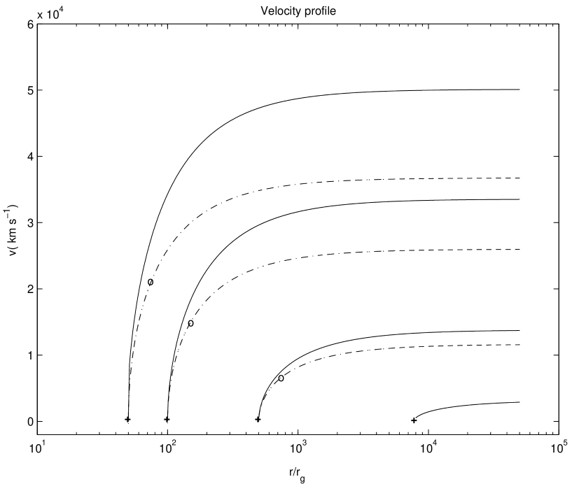
Figure 1: Solution of the wind equation  (19). Solid line - GEF solution, dashed line - CAK solution. Crosses indicate GEF critical points, circles - CAK critical points. Curves for $x=8000$ are graphically indistinguishable.

We step out from the critical point $x_{c}$ by means of the approximate formulas: $v=1\pm\mid p_{c}\mid\Delta x$, where $\Delta x=x-x_{c}$. On every integration step equation  (19) is solved numerically in order to obtain $dv/dx$. The forth order, adaptive Runge-Kutta scheme was used to obtain solutions depicted on Figure 1. - Figure 4.

Adjusting $x^{\rm CAK}_{c}$, $x^{\rm GEF}_{c}$ we select those solutions which both satisfy inner density condition. The following densities at the inner boundaries were adopted: $\rho_{in}=10^{-12}{\rm\,g\,cm^{-3}}$ for $x_{c}=50$, $\rho_{in}=10^{-14}{\rm\,g\,cm^{-3}}$ for $x_{c}=100$, $\rho_{in}=10^{-16}{\rm\,g\,cm^{-3}}$ for $x_{c}=500$, $\rho_{in}=10^{-21}{\rm\,g\,cm^{-3}}$ for $x_{c}=8000$. The comparative results of the numerical integration of  (19) for $s=1$ (GEF solution) and for $s=0$ (CAK wind theory) are shown on Fig.1. These solutions were obtained for the following set of parameters:

$x_{c}^{\rm GEF}$	$x_{c}^{\rm CAK}$	$v^{\infty}_{\rm GEF}\,\frac{\rm cm}{\rm s}$	$v^{\infty}_{\rm CAK}\,\frac{\rm cm}{\rm s}$	${\dot{M}}_{\rm GEF}\,\frac{\rm g}{\rm s}$	${\dot{M}}_{\rm CAK}\,\frac{\rm g}{\rm s}$
$50$	$75$	$5\cdot 10^{9}$	$3.67\cdot 10^{9}$	$2.56597\cdot 10^{26}$	$2.55692\cdot 10^{26}$
$100$	$155.2$	$3.3\cdot 10^{9}$	$2.6\cdot 10^{9}$	$2.56597\cdot 10^{26}$	$2.55693\cdot 10^{26}$
$500$	$751.7$	$1.37\cdot 10^{9}$	$1.15\cdot 10^{9}$	$2.56599\cdot 10^{26}$	$2.55697\cdot 10^{26}$

The difference between GEF and CAK wind is more pronounced when the considerable portion of the wind is accelerated at a distance less than $100\,r_{g}$ from BH. Note that the terminal velocity changes form $\Delta v^{\infty}/v^{\infty}=0.36$ for $x_{c}=50$ to $\Delta v^{\infty}/v^{\infty}=0.19$ for $x_{c}=500$. The obtained results show that the GEF flow can be sufficiently more fast than the flow which is described by CAK theory.

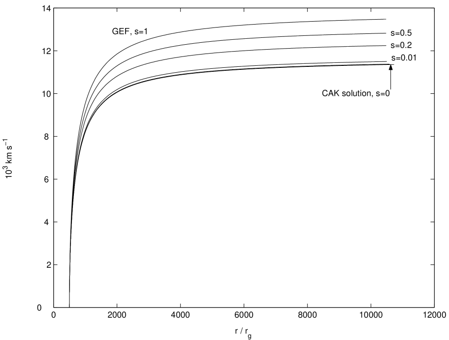
Figure 2: The continuous transition of the solution of  (19) from GEF (s=1) to CAK regime (s=0), see explanations in the text.

It is illustrative to demonstrate that CAK solution may be obtained from  (17) by ”switching off” smoothly the gravitational redshifting. To obtain the continuous transition from the GEF solution to the CAK solution of equation  (17) the following procedure was adopted. We assumed that the radiation force in  (17) is ${\displaystyle f_{L}\sim dv/dr+\frac{1}{c}\,s\,GM/r^{2}}$ The introduced parameter $s$ continuously changes from 1 (GEF case) to 0 (CAK wind). Numerically calculating solutions of  (17) for different values of $s$, applying the inner density boundary conditions it is possible to demonstrate the continuous transition of these solutions from the limiting cases of CAK and GEF solutions. The results are shown on Figure 2.

The introduction of the Paczynski - Wiita ( PW )  (16) potential, allows to simulate the effects of general relativity. Equations analogous to  (19),  (25),  (26) are derived in Appendix. The results of the numerical integration are shown on Figure 4. Introduction of the modified potential can give a gain in $v^{\infty}$ that varies from $\Delta v^{\infty}/v^{\infty}\sim 0.1$ for $x_{c}=30$ to $\Delta v^{\infty}/v^{\infty}\sim 0.03$ for $x_{c}=100$.

Approximate relations for $a_{1}$, $p_{c}$.

Introducing the following nondimmentional combination ${\displaystyle\epsilon=\frac{a}{c}}$, equation  (25) will read:

$$4a_{1}x_{c}^{2}\epsilon p_{c}^{2}+(a_{1}^{2}-1)p_{c}-4a_{1}\epsilon=0\mbox{.}$$ (27)

To obtain an approximate solution of  (27) we take into account that $\epsilon<<1$. Equation  (27) has two roots:

$$(p_{c})^{\pm}\simeq\frac{1}{8a_{1}\epsilon x_{c}^{2}}\left[1-a_{1}^{2}\pm(1-a_{1}^{2})\left(1+\frac{32a_{1}^{2}x_{c}^{2}\epsilon^{2}}{(a_{1}^{2}-1)^{2}}\right)\right]\mbox{.}$$ (28)

From  (28) we obtain

$$p_{c,1}\simeq-\frac{4a_{1}\epsilon}{1-a_{1}^{2}}\mbox{,}\qquad p_{c,2}\simeq\frac{1-a_{1}^{2}}{4a_{1}x_{c}^{2}\epsilon}\mbox{.}$$ (29)

We are looking for the solution with $p_{c}>0$ and with $a_{1}=a_{1}/v_{cr}<1$, thus the second root of  (29) should be considered:

$$p\simeq\frac{1}{4a_{1}x_{c}^{2}\epsilon}\mbox{,}$$ (30)

where it was supposed that $a_{1}<<1$. The accuracy of  (30) is $\Delta p_{c}/p_{c}\sim 10^{-3}$ (for $x_{c}=1$, $p_{c}=12.0027$, $p^{appox}_{1}=12.0169$).

To obtain an approximate relation for $a_{1}$ we substitute $p_{c,2}$ from  (29) to  (26). Taking into account that $\beta=a_{1}/\epsilon$, the resulting equation reads:

$$-2a_{1}^{2}x_{c}\epsilon^{2}+\frac{\alpha-1}{\alpha}\frac{(1-a_{1}^{2})^{2}}{4a_{1}}\epsilon+\frac{a_{1}^{2}(1-\Gamma)}{2}-\frac{\epsilon a_{1}}{2\alpha}(1-a_{1}^{2})=0\mbox{.}$$ (31)

Neglecting in  (31) terms which contain $a_{1}^{4}$ and $a_{1}^{3}\epsilon^{2}$ will result in the following equation for determining $a_{1}$:

$$2a_{1}^{3}(1-\Gamma)-2a_{1}^{2}\epsilon+\frac{\alpha-1}{\alpha}\epsilon=0\mbox{.}$$ (32)

The second term in  (32) is small compared with other two. It allows to obtain the following simple relation for $a_{1}$:

$$a_{1}\simeq\left(\frac{\epsilon}{2(1-\Gamma)}\frac{1-\alpha}{\alpha}\right)^{1/3}\mbox{.}$$ (33)

Calculating numerically $a_{1}$, $p_{c}$, from  (25), (26) we have found that the value of $a_{1}$ depends rather weakly on $x_{c}$: $x_{c}=50$, $a_{1}=0.034347$, $p_{c}=48.0109$; $x_{c}=500$, $a_{1}=0.034348$, $p_{c}=0.480112$; $x_{c}$=5000, $a_{1}=0.034369$, $p_{c}=0.004806$; (obtained for $\alpha=0.6$, $\Gamma=0.5$). Relation  (33) has a relatively good accuracy: for $\epsilon=6\cdot 10^{-5}$ (33) gives $a^{appr}_{1}\simeq 0.03430$ with accuracy $\Delta a_{1}/a_{1}=10^{-3}$. Velocity of the wind at the critical point is approximately $30\,a_{s}$ ($v_{c}=a_{1}^{-1}a_{s}$).

Above the critical point the influence of the $d\phi/dr$ (GEF) on the additional acceleration of the radiationally driven wind is small compared to the effect due to $dv/dr$.

3 Discussion

The most successive model describing winds from hot stars presented so far is that of Castor (1970), Castor,Abbott & Klein (1975). Geometry and ionization balance differ O-star wind from AGN outflow. Line driven wind from O-type star is spherically-symmetric. Outflows in AGN are assumed to be originated from the luminous accretion discs and approximately axially-symmetric. Powerful X-ray and UV radiation from the disc pose a problem of overionization of the outflowing plasma. In Sobolev approximation, which is in the background of the CAK theory, the radially streaming radiation flux is absorbed in a line transition in a wind with the gradually increasing velocity. A photon, emitted by a disc will be red-shifted due to Doppler effect. The resultant Sobolev optical depth $\tau_{l}\sim(dv/dr)^{-1}$. As it was shown by CAK, the radiation force that is due to an ensemble of optically thin and optically thick lines is proportional to $(dv/dr)^{\alpha}$. The more $dv/dr$ the more effectively a line is shifted to the powerful continuum. In a number of studies, CAK theory was applied to AGN in order to explain fast (up to $\sim 0.1c$) outflows Arav & Li (1994), Arav, Li & Begelman (1994), Murray at al. (1995), Proga et al. (1998), Proga et al. (2000). The CAK theory was enhanced by adopting axial symmetry. Ionization balance was studied in details simultaneously with 2D hydrodymanical calculations.

In this paper we developed a theory of winds that takes into account effects of the strong gravitational fields. We point out that if a wind is accelerated near super-massive BH a gravitational change of photon’s frequency must be taken into account. In a strong gravitational field a photon, emitted by a disc, will be red-shifted due to both the Doppler effect $\sim v/c$ and gravitational redshifting $\Delta\nu/\nu=\Delta\phi/c^{2}$. We argue that taking into account gravitational redshifting can substantially change the wind dynamics and structure. Although it should be mentioned that the developed theory (in the adopted toy model) cannot be directly applied to explain outflows from close to BH. An exact self-consistent solution of this problem is possible only in general relativity. We avoid this sophisticated task by considering all equations in flat space and time.

Basing on considerations of Sobolev we conclude that the greater $d\phi/dr$ the more effectively a line is shifted to the extent where the radiation flux is unattenuated. In such a case gravitational field ”exposes” a wind to the unattenuated continuum. Note that this effect is independent of the wind dynamics, it works also in a medium with $v=0$. We determine a wind accelerated in this regime: ”Gravitationally Exposed Flow” (GEF).

The main goal of this paper has been to compare a solution for GEF with that obtained from a standard line driven wind theory ( CAK ). To solve this problem a very simple input physics was assumed: spherical symmetry, constant temperature and no ionization balance. We found that in such a case the radiation force $f_{l}\sim(dv/dr+\frac{1}{c}d\phi/dr)^{-1}$. Numerical analysis shows that the introduced effect changes drastically a slope of a solution curve at the bottom of the wind. It is clearly a result of the fact that the role of the gravitational field is important when the field is high an velocity gradient is low. As soon as $dv/dr$ becomes sufficient, Sobolev effect efficiently stimulates the acceleration of the wind. Obtained equation of motion is nonlinear with respect to $dv/dr$ but this nonlinearity is different form that of CAK. Critical point of the equation of motion is neither a sonic point nor a CAK critical point. The position of the critical point $r_{c}$ is the only free parameter of the problem. Adjusting $r_{c}$ in order to satisfy density boundary conditions we compared solution for GEF with that of CAK which was obtained for the same physical and boundary conditions. Numerically solving equations describing spherical symmetric, stationary outflowing wind we found that gravitational redshifting can make acceleration up to $35\%$ (for $r_{cr}=50\,r_{g}$) more efficient.

In order to take approximately into account effects of general relativity, we made use of modified potential (Paczynski-Wiita potential). Numerical analysis demonstrated that if the critical point is located as far as $30\,r_{g}\div 100\,r_{g}$ the difference between PW case and Newtonian case is $\Delta v^{\infty}/v^{\infty}=0.1\div 0.03$

Acknowledgements Author is deeply grateful to G.S. Bisnovatyi-Kogan for continuous and stimulating attention to this work.

4 Conclusions

1. A theory of winds accelerated by the radiation pressure in lines with account of gravitational redshifting of photons is developed. A system of equations describing stationary, spherically-symmetric, isothermal flow is derived.

2. A solution of these equations is obtained numerically for two cases: a standard line-driven wind (CAK theory), Gravitationally Exposed Flow (GEF)- a wind that is accelerated by the radiation pressure in lines if to take into account gravitational redshifting. It is shown that an increase of up to $35\%$ in $v^{\infty}$ can be obtained.

3. To take approximately into account effects of general relativity, Paczynski - Wiita potential is adopted. A wind solution is calculated for this type of potential and comparative analysis with Newtonian case is presented.

4. The developed theory can be used to explain fast outflows from AGN.

Abbott D. 1980, ApJ, 242, 1183

Arav N., Korista, K.T., Martijn de Kool 2002, ApJ, 566, 699

Arav N., Li Z.Y. 1994, ApJ, 427, 700

Arav N., Li Z.Y., Begelman M.C. 1994, ApJ, 432, 62

Artemova I.V., Bjornsson G., Novikov I.D. 1996, ApJ, 456, 119a

Bisnovatyi-Kogan G.S., Dorodnitsyn A.V. 1999 A&A, 344, 647

Bisnovatyi-Kogan G.S. 2001, Stellar Physics, Vol.2, Springer, 2001

Castor J.I. 1970, MNRAS, 149, 111

Castor J.I., Abbott D.C, Klein R. 1975, ApJ, 195, 157

Landau L.D., Lifshitz E.M. 1960, The Classical Theory of Fields, New York: Pergamon

Lucy L.B., Solomon P. 1970, ApJ, 159, 879

Murray N., Chiang J., Grossman S.A., Voit G.M. 1995, ApJ, 451, 498

Proga D., Stone J.M., Drew J.E. 1998, MNRAS, 295, 595

Proga D., Stone J.M., Kallman T.R. 2000, ApJ, 543, 686

Stevens I.R., Kallman T.R. 1990, ApJ, 365, 321

Sobolev V.V. 1960, Moving envelopes of stars, Cambridge: Harvard University Press

Tennant, A.F., Mushotzky, R.F., Boldt, E.A. and Swank, J.H. 1981, ApJ, 251, 15

5 Appendix

Substituting Paczynski - Wiita potential into equation  (15) will obtain equation of motion:

$$F = \left(1-\frac{a}{v^{2}}\right)v\frac{dv}{dr}-\frac{2a^{2}}{r}+\frac{GM}{(r-r_{g})^{2}}-\frac{L\sigma}{4\pi r^{2}c}$$ (34)

$$- \frac{L\sigma k}{4\pi r^{2}c}\left(\frac{4\pi}{|{\dot{M}}|\sigma v_{th}}\right)^{\alpha}\left[vr^{2}\left(\frac{dv}{dr}+\frac{1}{c}\frac{GM}{(r-r_{g})^{2}}\right)\right]^{\alpha}=0\mbox{,}$$

Scaling all variables according to  (18), omiting tilda, equation  (34) reads:

$$F(p,v,x)=\left(1-\frac{a^{2}_{1}}{v^{2}}\right)vpx^{2}-2a_{1}^{2}x+\frac{\beta^{2}}{2}\left(\frac{x^{2}}{(x-1)^{2}}-\Gamma\right)$$

$$-\mu\beta^{2}\left[\frac{v}{\beta^{2}}\left(p+\frac{\beta}{2(x-1)^{2}}\right)\right]^{\alpha}=0\mbox{,}$$ (35)

where $p\equiv dv/dx$, $\mu$ is determined by  (21) and $a_{1}$, $\beta$ by  (20). Making use of  (22) and  (23) will result in the following relations:

$$\frac{\alpha-1}{\alpha}(1-a_{1}^{2})x_{c}^{2}p_{c}-2a_{1}^{2}x_{c}+\frac{\beta^{2}}{2}(\frac{x_{c}^{2}}{(x_{c}-1)^{2}}-\Gamma)-(1-a_{1}^{2})\frac{\beta}{2\alpha}\frac{x_{c}^{2}}{(x_{c}-1)^{2}}=0\mbox{,}$$ (36)

$$c_{2}p_{c}^{2}+c_{1}p_{c}+c_{0}=0\mbox{.}$$ (37)

Coefficients $c_{i}$ are determined from the following relations:

$$c_{2} = 2a_{1}^{2}x_{c}^{2}\mbox{,}$$ (38)

$$c_{1} = \frac{(a_{1}^{2}-1)x_{c}^{2}\beta}{2(x_{c}-1)^{2}}\mbox{,}$$ (39)

$$c_{0} = \frac{-x_{c}(\beta-1)\beta+a_{1}^{2}(-2(x_{c}-1)^{3}-\beta x_{c})}{(x_{c}-1)^{3}}\mbox{.}$$ (40)

Equation for $\mu$ reads:

$$\mu=\alpha^{-1}(1-a_{1}^{2})\left[\frac{x_{c}^{2}}{\beta^{2}}\left(p_{c}+\frac{\beta}{2(x_{c}-1)^{2}}\right)\right]^{1-\alpha}\mbox{.}$$ (41)

Equation  (41) is analoguis to  (24) except the last term in brackets. For a given $x_{c}$, equations  (36), (37) are solved numerically to determine $p_{c}$ and $a_{1}$. Then  (35) is integrated numerically as described in the text. Comparative results of the numerical solution of  (35) are depicted of Figure 4.

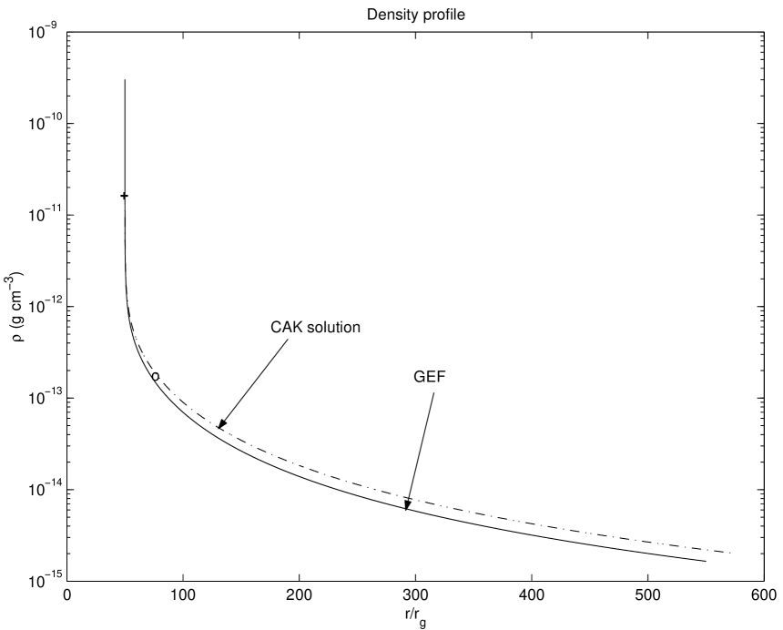
Figure 3: Density distribution in the wind. The solution curves calculated for $x^{GEF}_{c}=50$, $x^{GEF}_{c}=75$.

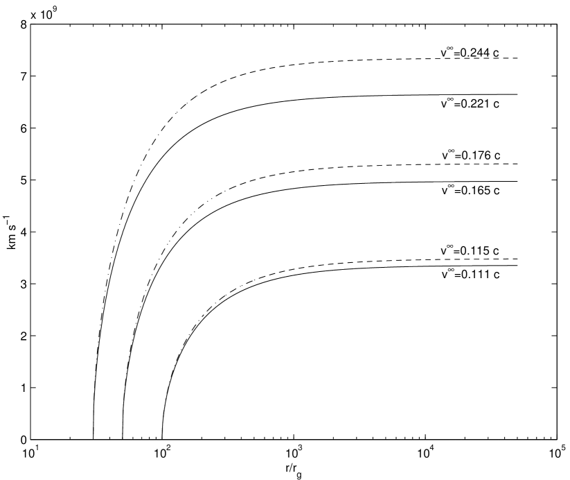
Figure 4: Solid line indicates GEF solution for the Newtonian potential, dashed line GEF solution for Paczynski - Wiita potential.