Effect of rotation on a developed turbulent stratified convection: the hydrodynamic helicity, the alpha-effect and the effective drift velocity

Abstract

An effect of rotation on a developed turbulent stratified convection is studied. Dependencies of the hydrodynamic helicity, the alpha-tensor and the effective drift velocity of the mean magnetic field on the rate of rotation and an anisotropy of turbulent convection are found. It is shown that in an anisotropic turbulent convection the alpha-effect can change its sign depending on the rate of rotation. The evolution of the alpha-effect is much more complicated than that of the hydrodynamic helicity in an anisotropic turbulent convection of a rotating fluid. Different properties of the effective drift velocity of the mean magnetic field in a rotating turbulent convection are found: (i) a poloidal effective drift velocity can be diamagnetic or paramagnetic depending on the rate of rotation; (ii) there is a difference in the effective drift velocities for the toroidal and poloidal magnetic fields; (iii) a toroidal effective drift velocity can play a role of an additional differential rotation. The above effects and an effect of a nonzero divergence of the effective drift velocity of the toroidal magnetic field on a magnetic dynamo in a developed turbulent stratified convection of a rotating fluid are studied. Astrophysical applications of the obtained results are discussed.

I Introduction

Turbulent transport of particles and magnetic fields was intensively studied for the Navier-Stokes turbulence (see, e.g., MY75 ; ZMR88 ; ZRS90 ; F95 ). However, there are a number of applications with other kinds of turbulence, e.g., turbulent convection. For instance, in the Sun and stars there is a developed turbulent convection that is strongly influenced by a fluid rotation.

The mean-field theory of magnetic field was in general developed for the Navier-Stokes turbulence without taking into account turbulent convection (see, e.g., M78 ; P79 ; KR80 ; ZRS83 ; RSS88 ; S89 ; RS92 ; R94 ). In particular, the dependencies of the the $\alpha$-effect, the effective drift velocity and the turbulent magnetic diffusion on the rate of rotation were found only for the Navier-Stokes turbulence (see, e.g., K91 ; RK93 ; KPR94 ; RKR00 ) in spite of that in many astrophysical applications there are turbulent convection regions. A turbulent convection in different situations has been studied mainly by numerical simulations (see, e.g., ZB89 ; BN90 ; TB97 ; BGT98 ; B2000 ; OSB01 ; OSB02 ).

In this paper we study an influence of rotation on a developed turbulent stratified convection. This allows us to find the dependencies of the hydrodynamic helicity, the alpha-tensor and the effective drift velocity of the mean magnetic field on the rate of rotation.

This study has a number of applications in astrophysics. In particular, the evolution of the mean magnetic field in the kinematic approximation (without taking into account a two-way coupling of mean magnetic field and turbulent fluid flow) can be described in terms of propagating waves with the growing amplitude, i.e., the magnitude of the mean magnetic field $B$ is given by

$$B\propto B_{0}\exp(\gamma_{{}_{B}}t)\cos(\omega_{{}_{B}}t+{\bf k}\cdot{\bf r})\;,$$ (1)

where $B_{0}$ is a seed magnetic field, $\gamma_{{}_{B}}$ is the growth rate of the mean magnetic field, $\omega_{{}_{B}}$ and ${\bf k}$ are the frequency and the wave vector of a dynamo wave. In the Sun, e.g., according to the magnetic field observations these dynamo waves with the $\sim 22$ years period propagate to the equator (see, e.g., M78 ; P79 ; KR80 ; ZRS83 ; S89 ). The magnetic field is generated in the turbulent convective zone inside the Sun. The growth of the mean magnetic field is a combined effect of a nonuniform fluid rotation (the differential rotation, $\mbox{\boldmath$\nabla$}(\delta\Omega))$ and helical turbulent motions (the $\alpha$-effect). The direction of propagation of the dynamo waves is determined by a sign of the parameter $\alpha[\partial(\delta\Omega)/\partial r],$ where $r,\theta,\varphi$ are the spherical coordinates, and ${\bf\Omega}$ is the angular velocity. When the parameter $\alpha\,[\partial(\delta\Omega)/\partial r]$ is negative the dynamo waves propagates to the equator. The helioseismology shows that in the solar convective zone $\partial(\delta\Omega)/\partial r>0$ and the existing theories yield $\alpha>0.$ This results in that the dynamo waves should propagate to the pole in contradiction to the solar magnetic field observations (see, e.g., M78 ; P79 ; KR80 ; ZRS83 ; S89 ).

In this study we found that in a developed turbulent convection the $\alpha$-effect can change its sign depending on the rate of rotation and an anisotropy of turbulence. In the lower part of the solar convective zone the fluid rotation is very fast in comparison with the turnover time of turbulent eddies. In this region $\alpha>0.$ In the upper part of the solar convective zone the fluid rotation is very slow and $\alpha<0.$ This explains the observed properties of the solar dynamo waves. The growth of the mean magnetic field is saturated by nonlinear effects (see, e.g., KRR94 ; F99 ; KR99 ; RK2000 ; KMRS2000 ). The $22$-years solar magnetic activity is also poorly understood. A characteristic time of the turbulent magnetic diffusion in the solar convective zone is of the order 2-3 years and it cannot explain the characteristic time of solar magnetic activity. We found that the fast rotation causes an additional effective drift velocity of a mean magnetic field that can increase the period of the dynamo waves provides the $22$-years solar magnetic activity.

II The governing equations and the method of the derivations

Our goal is to study an effect of rotation on a developed turbulent stratified convection. This allows us to derive dependencies of the hydrodynamic helicity, the alpha-effect and the effective drift velocity of the mean magnetic field on the angular velocity. To this end we consider a fully developed turbulent convection in a stratified rotating fluid with large Rayleigh and Reynolds numbers. The governing equations are given by

$${D{\bf u}\over Dt} = -\mbox{\boldmath$\nabla$}\biggl{(}{P\over\rho_{{}_{0}}}\biggr{)}+2{\bf u}\times{\bf\Omega}-{\bf g}S+{\bf f}_{\nu}\;,$$ (2)

$${DS\over Dt} = -{\bf u}\cdot{\bf N}_{b}-{1\over T_{0}}\,\mbox{\boldmath$\nabla$}\cdot{\bf F}_{\kappa}(S)\;,$$ (3)

where ${\bf u}$ is the fluid velocity with $\mbox{\boldmath$\nabla$}\cdot{\bf u}={\bf\Lambda}\cdot{\bf u},$ $\quad D/Dt=\partial/\partial t+{\bf u}\cdot\mbox{\boldmath$\nabla$},$ $\quad{\bf\Omega}$ is the angular velocity, ${\bf g}$ is the gravity field that includes an effect of the centrifugal force, $\rho_{{}_{0}}{\bf f}_{\nu}$ is the viscous force, ${\bf F}_{\kappa}(S)$ is the thermal flux that is associated with the molecular thermal conductivity, ${\bf\Lambda}=-\rho_{{}_{0}}^{-1}\mbox{\boldmath$\nabla$}\rho_{{}_{0}},$ $\quad{\bf N}_{b}=(\gamma P_{0})^{-1}\mbox{\boldmath$\nabla$}P_{0}-\rho_{{}_{0}}^{-1}\mbox{\boldmath$\nabla$}\rho_{{}_{0}}.$ The variables with the subscript $"0"$ corresponds to the hydrostatic equilibrium (i.e., the hydrostatic basic reference state):

$$\mbox{\boldmath$\nabla$}P_{0}=\rho_{{}_{0}}{\bf g}\;,$$ (4)

and $T_{0}$ is the equilibrium fluid temperature, $S=P/\gamma P_{0}-\rho/\rho_{{}_{0}}$ are the deviations of the entropy from the hydrostatic equilibrium, $P$ and $\rho$ are the deviations of the fluid pressure and density from the hydrostatic equilibrium. The Brunt-Väisälä frequency, $\tilde{\Omega}_{b},$ is determined by the equation $\tilde{\Omega}_{b}^{2}=-{\bf g}\cdot{\bf N}_{b}.$ To derive Eq. (2) we use an identity: $-\mbox{\boldmath$\nabla$}P+{\bf g}\rho=-\rho_{0}[\mbox{\boldmath$\nabla$}(P/\rho_{0})+{\bf g}S-P{\bf N}_{b}/\rho_{0}],$ where we assumed that $|P{\bf N}_{b}/\rho_{0}|\ll|{\bf g}S|,$ $\,|P{\bf N}_{b}/\rho_{0}|\ll|\mbox{\boldmath$\nabla$}(P/\rho_{0})|.$ This assumption corresponds to nearly isentropic basic reference state when ${\bf N}_{b}$ is very small. For the derivation of this identity we also used Eq. (4). We also consider a low-Mach-number fluid flow with a very small frequency $\tilde{\Omega}_{b},$ i.e., $|\tilde{\Omega}_{b}|\ll\sqrt{g\Lambda}$ and $|\tilde{\Omega}_{b}\tau|^{2}\ll 1,$ where $\tau$ is the correlation time of the turbulent velocity field. Equations (2) and (3) are written in the Boussinesq approximation for $\mbox{\boldmath$\nabla$}\cdot{\bf u}\not=0.$ This is more usually called ”the anelastic approximation”.

Now we consider a purely hydrostatic isentropic basic reference state, i.e., $\tilde{\Omega}_{b}=0$ $\,({\bf N}_{b}=0).$ Thus the turbulent convection is regarded as a small deviation from a well-mixed adiabatic state (for more discussion, see BR95 ). We will use a mean field approach whereby the velocity, pressure and entropy are separated into the mean and fluctuating parts. Using Eqs. (2) and (3) we derive equations for the turbulent fields: $v_{z}=\sqrt{\rho_{0}(z)}\,u_{z},$ $w=\sqrt{\rho_{0}(z)}\,(\mbox{\boldmath$\nabla$}{\bf\times}{\bf u})_{z}$ and $s=\sqrt{\rho_{0}(z)}\,(S-\bar{S}),$ where $\bar{S}\equiv\langle S\rangle$ is the mean entropy, the angular brackets denote ensemble averaging, and for simplicity we consider turbulent flow with zero mean velocity. Here $\rho_{0}(z)$ is dimensionless density measured in the units of $\rho_{0}(z=0).$ The equations for the turbulent fields are given by

$$\biggl{(}{\Lambda^{2}\over 4}-\Delta\biggr{)}{\partial v_{z}\over\partial t} = (2{\bf\Omega}\cdot\mbox{\boldmath$\nabla$}+{\bf\Omega}\cdot{\bf\Lambda})w+2\Lambda\Omega_{x}{\partial v_{z}\over\partial y}$$ (5)

$$-g\Delta_{\perp}s+V_{N}\;,$$

$${\partial w\over\partial t} = (2{\bf\Omega}\cdot\mbox{\boldmath$\nabla$}-{\bf\Omega}\cdot{\bf\Lambda})v_{z}+W_{N}\;,$$ (6)

$${\partial s\over\partial t} = -{\Omega_{b}^{2}\over g}v_{z}+S_{N}\;,$$ (7)

where $\Omega_{b}^{2}=-{\bf g}\cdot\mbox{\boldmath$\nabla$}\bar{S},$ $\,\Delta_{\perp}=\Delta-\partial^{2}/\partial z^{2},$ $\quad V_{N},$ $W_{N}$ and $S_{N}$ are the nonlinear terms which include the molecular dissipative terms [see Eqs. (53)-(55) in Appendix A], the field ${\bf g}$ is directed opposite to the axis $z$ and ${\bf\Omega}=(\Omega_{x},0,\Omega_{z}).$ We assumed here that $\Lambda^{-1}|\partial\Lambda/\partial z|\ll\Lambda.$ Equation (5) follows from Eq. (2) after the calculation $[\mbox{\boldmath$\nabla$}{\bf\times}(\mbox{\boldmath$\nabla$}{\bf\times}{\bf u})]_{z}.$

By means of Eqs. (5)-(7) we derive dependencies of the hydrodynamic helicity, the alpha-effect and the effective drift velocity on the angular velocity. The procedure of the derivation is outlined in the following (for details, see Appendixes A, B and C).

(a). Using Eqs. (5)-(7) we derive equations for the following second moments:

$$f_{ij}({\bf k}) = \hat{L}(v_{i},v_{j})\;,\quad\chi({\bf k})=\hat{L}(w,v_{z})\;,$$

$$F({\bf k}) = \hat{L}(s,w)\;,\quad G({\bf k})=\hat{L}(w,w)\;,$$

$$\Phi_{i}({\bf k}) = \hat{L}(s,v_{i})\;,\quad\Theta({\bf k})=\hat{L}(s,s)\;,$$

where $\hat{L}(a,b)=\langle a({\bf k})b(-{\bf k})\rangle$ and ${\bf v}=\sqrt{\rho_{0}(z)}\,{\bf u}.$ The equations for these correlation functions are given by Eqs. (47)-(52) in Appendix A. In this derivation we assumed that $\Lambda^{2}\ll k^{2}.$

(b). The equations for the second moments contain third moments and a problem of closing the equations for the higher moments arises. Various approximate methods have been proposed for the solution of problems of this type (see, e.g., MY75 ; O70 ; Mc90 ). The simplest procedure is the $\tau$ approximation, which is widely used in the theory of kinetic equations. For magnetohydrodynamic turbulence this approximation was used in PFL76 (see also RK2000 ; KRR90 ; KMR96 ). One of the simplest procedures which allows us to express the third moments $f_{{}_{N}},$ $\chi_{{}_{N}},\ldots,$ $\Theta_{N}$ in Eqs. (47)-(52) in terms of the second moments, reads

$$f_{{}_{N}}({\bf k})-f_{{}_{N}}^{(0)}({\bf k}) = -{f({\bf k})-f^{(0)}({\bf k})\over\tau(k)}\;,$$ (8)

and similarly for other third moments, where $f({\bf k})=e_{i}e_{j}f_{ij}({\bf k}),$ $\,{\bf e}$ is the unit vector directed along the axis $z,$ the superscript $(0)$ corresponds to the background turbulent convection (it is a turbulent convection without rotation, ${\bf\Omega}=0),$ and $\tau(k)$ is the characteristic relaxation time of the statistical moments. Note that we applied the $\tau$-approximation only to study the deviations from the background turbulent convection which is caused by the rotation. The background turbulent convection is assumed to be known.

The $\tau$-approximation is in general similar to Eddy Damped Quasi Normal Markowian (EDQNM) approximation. However, there is a principle difference between these two approaches (see O70 ; Mc90 ). The EDQNM closures do not relax to equilibrium, and this procedure does not describe properly the motions in the equilibrium state in contrast to the $\tau$-approximation. Within the EDQNM theory, there is no dynamically determined relaxation time, and no slightly perturbed steady state can be approached O70 . In the $\tau$-approximation, the relaxation time for small departures from equilibrium is determined by the random motions in the equilibrium state, but not by the departure from equilibrium O70 . As follows from the analysis performed in O70 the $\tau$-approximation describes the relaxation to the equilibrium state (the background turbulent convection) more accurately than the EDQNM approach.

Note that we analyzed the applicability of the $\tau$-approximation for description of the mean-field dynamics of the mean magnetic field and mean scalar fields by comparison of the derived mean-field equations using other methods such as the path-integral approach and the renormalization group approach (see KR94 ; RK97 ; EKR96 ; EKR97 ; EKRP97 . This comparison showed that the $\tau$-approximation yields the results similar to that obtained by means of the other methods.

(c). We assume that the characteristic times of variation of the second moments $f({\bf k}),$ $\chi({\bf k}),\ldots,$ $\Theta({\bf k})$ are substantially larger than the correlation time $\tau(k)$ for all turbulence scales. This allows us to determine a stationary solution for the second moments $f({\bf k}),$ $\chi({\bf k}),\ldots,$ $\Theta({\bf k})$ [see Eqs. (65)-(73) in Appendix A].

(d). For the integration in ${\bf k}$-space of the second moments $f({\bf k}),$ $\chi({\bf k}),\ldots,$ $\Theta({\bf k})$ we have to specify a model for the background turbulent convection (without rotation). Here we use the following model of the background turbulent convection which will be discussed in more details in Appendix D:

$$f_{ij}^{(0)}({\bf k}) = f_{\ast}\tilde{W}(k)[P_{ij}({\bf k})+\varepsilon P_{ij}^{(\perp)}({\bf k}_{\perp})]\;,$$ (9)

$$\Phi^{(0)}_{i}({\bf k}) = k_{\perp}^{-2}[k^{2}\Phi_{z}^{(0)}({\bf k})e_{j}P_{ij}({\bf k})$$ (10)

$$+iF^{(0)}({\bf k})({\bf e}{\bf\times}{\bf k})_{i}]\;,$$

$$\Phi_{z}^{(0)}({\bf k}) = \Phi^{\ast}_{z}\tilde{W}(k)\biggl{[}2\sigma-3(\sigma-1)\biggl{(}{k_{\perp}\over k}\biggr{)}^{2}\biggr{]}\;,$$ (11)

$$F^{(0)}({\bf k}) = -6i({\bf\Phi}^{\ast}\cdot({\bf e}{\bf\times}{\bf k}))f^{(0)}({\bf k})/f_{\ast}\;,$$ (12)

$$G^{(0)}({\bf k}) = (1+\varepsilon)f^{(0)}({\bf k})k^{2}\;,$$ (13)

$$\Theta^{(0)}({\bf k}) = 2\Theta_{\ast}\tilde{W}(k)\;,$$ (14)

where $f_{ij}({\bf k})=\langle v_{i}({\bf k})v_{j}(-{\bf k})\rangle,$ $\,\tilde{W}(k)=W(k)/8\pi k^{2},$ $\,f^{(0)}({\bf k})=f_{\ast}(k_{\perp}/k)^{2}\tilde{W}(k),$ and $f_{ij}^{(0)}({\bf k})e_{ij}=f^{(0)}({\bf k}),$

$$\varepsilon={2\over 3}\biggl{(}{\langle{\bf u}_{\perp}^{2}\rangle\over\langle{\bf u}_{z}^{2}\rangle}-2\biggr{)}$$

is the degree of anisotropy of the turbulent velocity field ${\bf u}={\bf u}_{\perp}+u_{z}{\bf e}.$ Here $P_{ij}({\bf k})=\delta_{ij}-k_{ij},$ $\,k_{ij}=k_{i}k_{j}/k^{2},$ $\,{\bf k}={\bf k}_{\perp}+k_{z}{\bf e},$ $\,k_{z}={\bf k}\cdot{\bf e},$ $\,P_{ij}^{(\perp)}({\bf k}_{\perp})=\delta_{ij}-k^{\perp}_{ij}-e_{ij},$ $\,k^{\perp}_{ij}=({\bf k}_{\perp})_{i}({\bf k}_{\perp})_{j}/k_{\perp}^{2},$ $\,e_{ij}=e_{i}e_{j},$ $\,\sigma$ is the degree of anisotropy of the turbulent flux of entropy (see below). We assume that $\tau(k)=2\tau_{{}_{0}}\bar{\tau}(k),$ $\,W(k)=-d\bar{\tau}(k)/dk,$ $\,\bar{\tau}(k)=(k/k_{0})^{1-q},$ $\,1<q<3$ is the exponent of the kinetic energy spectrum (e.g., $q=5/3$ for Kolmogorov spectrum), $k_{0}=1/l_{0},$ and $l_{0}$ is the maximum scale of turbulent motions, $\tau_{{}_{0}}=l_{0}/u_{0}$ and $u_{0}$ is the characteristic turbulent velocity in the scale $l_{0}.$ Motion in the background turbulent convection is assumed to be non-helical. In Eqs. (9) and (10) we neglected small terms $\sim O(\Lambda f_{\ast})$ and $\sim O(\Lambda\Phi^{\ast}_{z}),$ respectively. Now we calculate $f_{ij}^{(0)}\equiv\int f_{ij}^{(0)}({\bf k})\,d{\bf k}$ using Eq. (9): $f_{ij}^{(0)}=(f_{\ast}/3)[\delta_{ij}+(3\varepsilon/4)(\delta_{ij}-e_{ij})].$ Note that $-4/3\leq\varepsilon<\infty.$ The lower limit of $\varepsilon$ follows from the condition $f_{xx}^{(0)}\geq 0$ (or $f_{yy}^{(0)}\geq 0).$ Similarly, using Eqs. (10)-(12) we obtain ${\bf\Phi}^{(0)}\equiv\int{\bf\Phi}^{(0)}({\bf k})\,d{\bf k}={\bf\Phi}^{\ast}.$ The parameter $\sigma$ can be presented in the form

$$\sigma = {1+\tilde{\xi}(q+1)/(q-1)\over 1+\tilde{\xi}/3}\;,$$ (15)

$$\tilde{\xi} = (l_{\perp}/l_{z})^{q-1}-1\;,$$ (16)

where $l_{\perp}$ and $l_{z}$ are the horizontal and vertical scales in which the two-point correlation function $\Phi_{z}^{(0)}({\bf r})=\langle s({\bf x}){\bf u}({\bf x}+{\bf r})\rangle$ tends to zero. The parameter $\tilde{\xi}$ determines the degree of thermal anisotropy. In particular, when $l_{\perp}=l_{z}$ the parameter $\tilde{\xi}=0$ and $\sigma=1.$ For $l_{\perp}\ll l_{z}$ the parameter $\tilde{\xi}=-1$ and $\sigma=-3/(q-1).$ The maximum value $\tilde{\xi}_{\rm max}$ of the parameter $\tilde{\xi}$ is given by $\tilde{\xi}_{\rm max}=q-1$ for $\sigma=3.$ Thus, for $\sigma<1$ the thermal structures have the form of column or thermal jets $(l_{\perp}<l_{z}),$ and for $\sigma>1$ there exist the ‘’pancake” thermal structures $(l_{\perp}>l_{z})$ in the background turbulent convection.

The relationship between $\Phi^{\ast}_{z}$ and $f_{\ast}$ follows from Eq. (44) for the kinetic turbulent energy $\rho_{{}_{0}}\langle{\bf u}^{2}\rangle,$ and it is given by $f_{\ast}=2\lambda g\tau_{{}_{0}}\Phi^{\ast}_{z}/\varepsilon,$ where $\lambda=2\varepsilon\delta_{\ast}/(\varepsilon+2)$ and $\delta_{\ast}=(3-q)/2(q-1).$ Note that for Kolmogorov spectrum $q=5/3$ and $\delta_{\ast}=1.$ In Section III we will present results for $\delta_{\ast}=1.$ For the integration in ${\bf k}$-space we used identities given in Appendixes B and C.

Thus, the ”input parameters” in the theory include the parameters that describe the model of background turbulent convection, i.e., the degree of anisotropy of the turbulent velocity field $\varepsilon,$ the degree of anisotropy of the turbulent flux of entropy $\sigma,$ the maximum scale of turbulent motions $l_{0},$ the turbulent velocity $u_{0}\equiv\sqrt{\langle{\bf u}^{2}\rangle}=\sqrt{f_{pp}^{(0)}}$ (the r.m.s. velocity) in the maximum scale of turbulent motions, the exponent of the kinetic energy spectrum $q.$ The ”input parameters” also include the density stratification length $\Lambda$ and the angular velocity ${\bf\Omega}.$ Note that $f_{\ast}=u_{0}^{2}/(1+\varepsilon/2)$ and $\Phi^{\ast}_{z}=u_{0}^{2}/(2\delta_{\ast}g\tau_{{}_{0}}).$ The described above procedure allows us to determine the dependencies of the hydrodynamic helicity, the alpha-effect and the effective drift velocity of the mean magnetic field on the rate of rotation.

The considered model of a background turbulent convection written in ${\bf k}$-space is enough general and it does not contradict to the known Nusselt number dependencies on Rayleigh number. On the other hand, the observations of the turbulent convection on the surface of the Sun cannot give the Nusselt number dependence on Rayleigh number, i.e., it is possible to obtain only one point in this curve. The parameters $\varepsilon,$ $\,u_{0},$ $\,l_{0},$ ${\bf\Omega},$ etc can be calculated from the solar observations. In addition, the direct numerical simulations of turbulent convection (see BN90 ; OSB01 ; OSB02 ) are in an agreement with our model of turbulent convection.

III Effect of rotation

In this Section we present the results of the calculations (described above) for the hydrodynamic helicity, the alpha-effect and the effective drift velocity of the mean magnetic field as the functions of the rate of rotation and an anisotropy of turbulence.

III.1 The hydrodynamic helicity

Using Eqs. (77) and (81) in Appendix A we find the dependence of the hydrodynamic helicity $\chi^{(v)}=\langle{\bf u}~{}\cdot~{}(\mbox{\boldmath$\nabla$}{\bf\times}{\bf u})\rangle$ on the angular velocity:

$$\chi^{(v)} = -{1\over 12}\biggl{(}{l_{0}^{2}\Omega\over L_{\rho}\tau_{{}_{0}}}\biggr{)}\,[\Psi_{1}(\omega)+\Psi_{2}(\omega)\sin^{2}\phi_{l}$$ (17)

$$+\Psi_{3}(\omega)\sin^{4}\phi_{l}]\sin\phi_{l}\;$$

(for details, see Appendix A), where $\omega=4\tau_{{}_{0}}\Omega,$ $\,l_{0}=u_{0}\tau_{{}_{0}},$ $\,u_{0}^{2}=2g\tau_{{}_{0}}\Phi^{\ast}_{z}\delta_{\ast},$ $\,\sin\phi_{l}=\mbox{\boldmath$\hat{\omega}$}\cdot{\bf e},$ $\,\phi_{l}$ is the latitude, $\,\mbox{\boldmath$\hat{\omega}$}={\bf\Omega}/\Omega,$ $\,{\bf e}$ is the unit vector directed along the $z$-axis, $\,L_{\rho}=\Lambda^{-1},$ the functions $\Psi_{m}(\omega)$ are given by Eqs. (137) in Appendix C. Hereafter we assume that $\delta_{\ast}=1.$ For a slow rotation $(\omega\ll 1)$ the hydrodynamic helicity $\chi^{(v)}$ is given by

$$\chi^{(v)}\approx-{1\over 6}\biggl{(}{l_{0}^{2}\Omega\over L_{\rho}\tau_{{}_{0}}}\biggr{)}\sin\phi_{l}\left({164\sigma\over 15}+{12\over 5}-5\lambda\right)\;,$$ (18)

and for $\omega\gg 1$ it is given by

$$\chi^{(v)}\approx{3\pi\over 8}\biggl{(}{l_{0}u_{0}\over L_{\rho}\tau_{{}_{0}}}\biggr{)}\lambda\biggl{(}1+{1\over 4}\sin^{2}\phi_{l}\biggr{)}\sin\phi_{l}\;.$$ (19)

Note that the meaning $\omega\equiv 4\Omega\tau_{{}_{0}}\gg 1$ is $\omega$ large, but only up to some upper limit, i.e., an intermediate range of values. This implies that the rotation cannot be very fast to affect the correlation time $\tau(k)$ of turbulent velocity field in its inertial range. Also we assumed that the parameters $\varepsilon$ and $\sigma$ are independent of $\omega.$

III.2 The $\alpha$-effect

Now we find the dependence of the $\alpha$-effect on the angular velocity. To this end we use the induction equation for the magnetic field

$${\partial{\bf H}\over\partial t}=\mbox{\boldmath$\nabla$}\times({\bf u}\times{\bf H}-\eta\mbox{\boldmath$\nabla$}\times{\bf H})\;,$$ (20)

where $\eta$ is the magnetic diffusion due to the electrical conductivity of fluid. The magnetic field, ${\bf H}$, is divided into the mean and fluctuating parts: ${\bf H}={\bf B}+{\bf b},$ where the mean magnetic field ${\bf B}=\langle{\bf H}\rangle$ and ${\bf b}$ is the fluctuating field. An equation for ${\bf h}=\sqrt{\rho_{0}}\,{\bf b}$ follows from Eq. (20) and it is given by

$${\partial{\bf h}\over\partial t} = ({\bf B}\cdot\mbox{\boldmath$\nabla$}){\bf v}-({\bf v}\cdot\mbox{\boldmath$\nabla$}){\bf B}-({\bf v}\cdot{\bf\Lambda}){\bf B}$$ (21)

$$+{1\over 2}({\bf B}\cdot{\bf\Lambda}){\bf v}+{\bf H}_{N}\;,$$

where ${\bf H}_{N}$ are the nonlinear terms which also include the magnetic diffusion term [see Eq. (90) in Appendix A]. In order to derive equation for the $\alpha$-tensor we introduce the electromotive force ${\cal E}_{i}=\langle{\bf u}\times{\bf b}\rangle_{i}=\rho_{0}^{-1}\varepsilon_{imn}\int\chi^{(c)}_{mn}({\bf k})\,d{\bf k},$ where $\chi^{(c)}_{ij}({\bf k})=\langle v_{i}({\bf k})h_{j}(-{\bf k})\rangle\equiv\hat{L}(v_{i},h_{j}).$ A general form of the electromotive force is given by ${\cal E}_{i}=\alpha_{ij}B_{j}+({\bf V}^{\rm eff}{\bf\times}{\bf B})_{i}-\eta_{ij}(\mbox{\boldmath$\nabla$}{\bf\times}{\bf B})_{j}-\kappa_{ijk}(\partial\hat{B})_{ij}-[\mbox{\boldmath$\delta$}{\bf\times}(\mbox{\boldmath$\nabla$}{\bf\times}{\bf B})]_{i}=a_{ij}B_{j}+b_{ijk}B_{i,j}$ (see, e.g., R80 and Appendix A), where the tensors $\alpha_{ij}$ and $\eta_{ij}$ describe the $\alpha$-effect and turbulent magnetic diffusion, respectively, ${\bf V}^{\rm eff}$ is the effective diamagnetic (or paramagnetic) velocity, $\kappa_{ijk}$ and $\delta$ describe a nontrivial behavior of the mean magnetic field in an anisotropic turbulence, $B_{i,j}=\nabla_{j}B_{i}$ and $(\partial\hat{B})_{ij}=(1/2)(B_{i,j}+B_{j,i}).$ The $\alpha$-tensor, $\alpha_{ij},$ is determined by a symmetric part of the tensor $a_{ij},$ i.e., by $a_{ij}^{(S)}\equiv(1/2)(a_{ij}+a_{ji}).$ The tensor $a_{ij}$ is calculated in Appendix A. The $\alpha$-tensor is given by

$$\alpha_{ij} = {1\over 6}\biggl{(}{l_{0}^{2}\Omega\over L_{\rho}}\biggr{)}\{\sin\phi_{l}\,[(\Psi_{4}(\omega)+\Psi_{5}(\omega)\sin^{2}\phi_{l})\,\delta_{ij}$$ (22)

$$+(\Psi_{6}(\omega)+\Psi_{7}(\omega)\sin^{2}\phi_{l})\,\omega_{ij}+\,\Psi_{8}(\omega)\,e_{ij}]$$

$$+[\Psi_{9}(\omega)+\Psi_{10}(\omega)\sin^{2}\phi_{l}]\,(e_{i}\hat{\omega}_{j}+e_{j}\hat{\omega}_{i})\}\;,$$

(for details, see Appendix A), where $\omega_{ij}=\hat{\omega}_{i}\hat{\omega}_{j},$ $\,e_{ij}=e_{i}e_{j},$ the functions $\Psi_{m}(\omega)$ are given by Eqs. (137) in Appendix C. Here we present asymptotic formulas for the isotropic part $(\alpha_{ij}^{({\rm isotr})}\equiv\alpha\delta_{ij})$ of the $\alpha$-tensor. For a slow rotation $(\omega\ll 1)$ the parameter $\alpha$ is given by

$$\alpha\approx{4\over 5}\biggl{(}{l_{0}^{2}\Omega\over L_{\rho}}\biggr{)}\biggl{(}2-{\sigma\over 3}-{5\lambda\over 6}\biggr{)}\sin\phi_{l}\;,$$ (23)

and for $\omega\gg 1$ it is given by

$$\alpha \approx -{\pi\over 32}\biggl{(}{l_{0}u_{0}\over L_{\rho}}\biggr{)}\biggl{(}2\lambda+{\sigma\over 3}-3$$ (24)

$$+(\sigma-1)\sin^{2}\phi_{l}\biggr{)}\sin\phi_{l}\;.$$

It is seen from Eqs. (18) and (23) that for a slow rotation and isotropic background turbulent convection $(\sigma=1$ and $\varepsilon=0),$ the parameter $\alpha\approx-(5/27)\tau_{{}_{0}}\chi^{(v)},$ where $\chi^{(v)}=\langle{\bf u}\cdot(\mbox{\boldmath$\nabla$}{\bf\times}{\bf u})\rangle.$ However, when a rotation is not slow, the latter relationship does not valid.

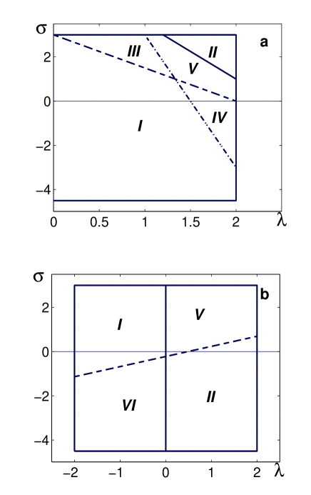
Figure 1: Characteristic ranges of parameters with different behavior of $\alpha$-effect (FIG.1a) and the parameter $\alpha_{\chi}=-(1/3)\tau_{{}_{0}}\chi^{(v)}$ (FIG.1b). The range I for the $\alpha$-effect (FIG.1a) also exists for $-2<\lambda<0$ and $-9/2<\sigma<3.$

The $\alpha$-effect depends on the degrees of the velocity anisotropy $\varepsilon$ and the thermal anisotropy $\sigma.$ Asymptotic formulas for a slow rotation $(\omega\ll 1)$ and for $\omega\gg 1$ show that there are several characteristic ranges of parameters with different behavior of $\alpha$-effect. In FIG. 1a these ranges are separated by lines $\sigma=3(3-2\lambda),$ $\,\sigma=3(1-\lambda/2)$ and $\sigma=6-5\lambda/2,$ where $-2<\lambda<2,$ $\,-9/2<\sigma<3,$ and $0\leq\phi_{l}\leq\pi/2.$ Here $\lambda=2\varepsilon/(\varepsilon+2).$ In the ranges I and II the $\alpha$-effect does not change its sign for all $\Omega\tau_{{}_{0}}$ and $\phi_{l}.$ In particular, in the range I: $\alpha>0$ and in the range II: $\alpha<0.$ In the range V the $\alpha$-effect changes its sign at a certain value of $\Omega\tau_{{}_{0}}$ for all $\phi_{l}.$ In the ranges III and IV the $\alpha$-effect changes its sign at a certain value of $\Omega\tau_{{}_{0}}$ and a certain range of the latitudes $\phi_{l}.$ In the range III the degree of thermal anisotropy $\sigma>1$ (which corresponds to the ”pancake” small-scale thermal structure of the background turbulent convection), and in the range IV the degree of thermal anisotropy $\sigma<1$ (i.e., a column-like thermal structure). The $\alpha$-effect can be negative for a slow rotation only in the range II. Note that the negative $\alpha$-effect corresponds to the propagation of the solar dynamo waves to the equator.

Our analysis shows that when the rotation is not slow, the $\alpha$-effect is determined not only by the contributions from the hydrodynamic helicity and its behavior is much more complicated in a rotating fluid. In order to demonstrate this we plotted in FIGS. 2-4 the dependencies of the $\alpha$-effect (solid line) and $\alpha_{\chi}\equiv-(1/3)\tau_{{}_{0}}\chi^{(v)}$ (dashed line) on the parameter $\Omega\tau_{{}_{0}}$ for different latitudes (FIG. 2 is for the latitude $\phi_{l}=15^{\circ},$ FIG. 3 is for $\phi_{l}=35^{\circ}$ and FIG. 4 is for $\phi_{l}=90^{\circ}).$ Here the parameters $\alpha$ and $\alpha_{\chi}$ are measured in the units of $l_{0}u_{0}/4L_{\rho}.$ Figures 2-4 demonstrate that the functions $\alpha(\Omega\tau_{{}_{0}})$ and $\alpha_{\chi}(\Omega\tau_{{}_{0}})$ are totally different. For example, in the case $\varepsilon=13$ and $\sigma=0$ the $\alpha$-effect and $\alpha_{\chi}$ have opposite signs for all $\Omega\tau_{{}_{0}}$ (see FIG. 4c).

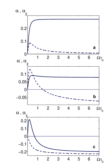
Figure 2: The $\alpha$ (solid line) and $\alpha_{\chi}=-(1/3)\tau_{{}_{0}}\chi^{(v)}$ (dashed line) as the functions of the parameter $\Omega\tau_{{}_{0}}$ for $\phi_{l}=15^{\circ}$ and different values of the degrees of anisotropy: (a). $\varepsilon=0$ and $\sigma=1$; (b). $\varepsilon=1.2$ and $\sigma=2$; (c). $\varepsilon=13$ and $\sigma=0.$ In FIG. 2c the $\alpha$ effect is multiplied by $5.$

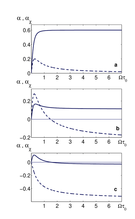
Figure 3: The $\alpha$ (solid line) and $\alpha_{\chi}=-(1/3)\tau_{{}_{0}}\chi^{(v)}$ (dashed line) as the functions of the parameter $\Omega\tau_{{}_{0}}$ for $\phi_{l}=35^{\circ}$ and different values of the degrees of anisotropy: (a). $\varepsilon=0$ and $\sigma=1$; (b). $\varepsilon=1.2$ and $\sigma=2$; (c). $\varepsilon=13$ and $\sigma=0.$

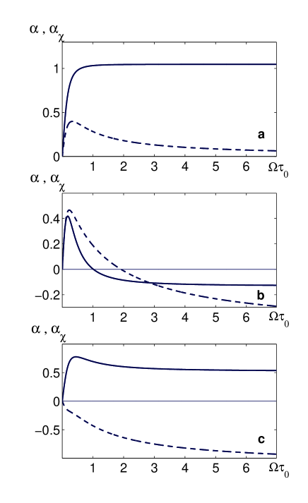
Figure 4: The $\alpha$ (solid line) and $\alpha_{\chi}=-(1/3)\tau_{{}_{0}}\chi^{(v)}$ (dashed line) as the functions of the parameter $\Omega\tau_{{}_{0}}$ for $\phi_{l}=90^{\circ}$ and different values of the degrees of anisotropy: (a). $\varepsilon=0$ and $\sigma=1$; (b). $\varepsilon=1.2$ and $\sigma=2$; (c). $\varepsilon=13$ and $\sigma=0.$ In FIG. 4b the $\alpha$ effect is multiplied by $2$ and in FIG. 4c by $5/2.$

Figure 1b shows the ranges of parameters $(\sigma$ and $\lambda)$ with different behavior of $\alpha_{\chi}.$ In FIG. 1b these ranges are separated by lines $\sigma=(9/41)(25\lambda/12-1)$ and $\lambda=0,$ where $-2<\lambda<2$ and $-9/2<\sigma<3.$ The numeration of the ranges in FIG. 1b for $\alpha_{\chi}$ is the same as for the parameter $\alpha$ in FIG. 1a. Comparison of FIGS. 1a and 1b shows that the ranges III and IV (whereby the $\alpha$-effect changes its sign at a certain value of $\Omega\tau_{{}_{0}}$ and a certain range of the latitudes $\phi_{l})$ do not exist for $\alpha_{\chi}.$ On the other hand, there is a new range (the range VI) in FIG 1b whereby the sign of $\alpha_{\chi}$ changes from negative value for a slow rotation to positive value for $\omega\gg 1.$ The locations of the ranges II and V for $\alpha_{\chi}$ are different from that of the $\alpha$-effect. Therefore, the behavior of the parameter $\alpha_{\chi}$ and the $\alpha$-effect are different in a rotating fluid.

The dependencies of the $\alpha$ effect on the latitude $\phi_{l}$ for different values of the degrees of anisotropy $\varepsilon$ and $\sigma$, and different values of the parameter $\Omega\tau_{{}_{0}}$ are shown in FIG. 5. It is seen in FIG. 5b that the $\alpha$ effect changes its sign at $\phi_{l}\approx 20^{\circ}-40^{\circ}$ for $\Omega\tau_{{}_{0}}=5$ (this value of $\Omega\tau_{{}_{0}}$ corresponds to the lower part of the solar convective zone).

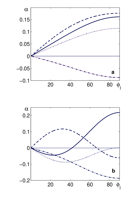
Figure 5: The dependence of the $\alpha$ effect on the latitude $\phi_{l}$ for different values of the degrees of anisotropy: $\varepsilon=1.2$ and $\sigma=2$ (dashed); $\varepsilon=13$ and $\sigma=0$ (solid); $\varepsilon=13$ and $\sigma=2.2$ (dashed-dotted); $\varepsilon=13$ and $\sigma=0.415$ (dotted); and for different values of the parameter $\Omega\tau_{{}_{0}}:$ (a). $\Omega\tau_{{}_{0}}=0.1$; (b). $\Omega\tau_{{}_{0}}=5.$ The dashed-dotted line in FIG. 5b shows $\alpha/5$. The latitude is measured in degrees.

In view of the applications to the astrophysics, the case with negative $\alpha$-effect for $\phi_{l}>0$ is most important because this provides a propagation of the solar dynamo waves to the equator according to the solar observations (see, e.g., M78 ; P79 ; KR80 ; ZRS83 ; S89 ).

III.3 The effective drift velocity of the mean magnetic field

Now we determine the effective drift velocity $V_{k}^{(d)}\equiv-(1/2)\varepsilon_{kij}a_{ij}^{(AS)}=V_{k}^{(1)}+V_{k}^{(2)}$ of the mean magnetic field using Eq. (112), where $a_{ij}^{(AS)}=(1/2)(a_{ij}-a_{ji}),$ and

$${\bf V}^{(1)} = {1\over 48}\biggl{(}{l_{0}u_{0}\over L_{\rho}}\biggr{)}\{{\bf e}[E_{1}(\omega)+E_{2}(\omega)\sin^{2}\phi_{l}$$ (25)

$$+E_{3}(\omega)\sin^{4}\phi_{l}]-{1\over 2}{\bf e}_{\theta}[E_{4}(\omega)$$

$$+E_{3}(\omega)\sin^{2}\phi_{l}]\sin(2\phi_{l})\}\;,$$

$${\bf V}^{(2)} = {1\over 6}\biggl{(}{l_{0}^{2}\Omega\over L_{\rho}}\biggr{)}[E_{5}(\omega)$$ (26)

$$+E_{6}(\omega)\sin^{2}\phi_{l}](\mbox{\boldmath$\hat{\omega}$}{\bf\times}{\bf e})\;.$$

(for details, see Appendix A), where $r,\theta,\varphi$ are the spherical coordinates, $\phi_{l}=\pi/2-\theta,$ $\,\mbox{\boldmath$\hat{\omega}$}{\bf\times}{\bf e}=\cos\phi_{l}\,{\bf e}_{\varphi},$ $\mbox{\boldmath$\hat{\omega}$}={\bf e}\,\sin\phi_{l}-{\bf e}_{\theta}\,\cos\phi_{l},$ the functions $E_{k}(\omega)$ are given in Appendix C. For a slow rotation $(\omega\ll 1)$ the effective drift velocities are given by

$${\bf V}^{(1)} \approx -{4\over 15}\biggl{(}{l_{0}u_{0}\over L_{\rho}}\biggr{)}\biggl{[}{\bf e}\biggl{(}1-{\sigma\over 6}+{5\over 4(\varepsilon+2)}$$ (27)

$$+O(\omega^{2})\biggr{)}-{\bf e}_{\theta}{5\over 12}\omega^{2}\biggl{(}1-{\sigma\over 6}$$

$$-{3\varepsilon-1\over 7(\varepsilon+2)}\biggr{)}\sin(2\phi_{l})\,\biggr{]}\;,$$

$${\bf V}^{(2)} \approx {4\over 5}\biggl{(}{l_{0}^{2}\Omega\over L_{\rho}}\biggr{)}\biggl{(}1-{\sigma\over 6}+{5(1-\varepsilon)\over 9(\varepsilon+2)}\biggr{)}(\mbox{\boldmath$\hat{\omega}$}{\bf\times}{\bf e})\;,$$ (28)

and for $\omega\gg 1$ they are given by

$${\bf V}^{(1)} \approx -{\pi\over 8\omega}\biggl{(}{l_{0}u_{0}\over L_{\rho}}\biggr{)}[{\bf e}(1+\sin^{2}\phi_{l})$$ (29)

$$-{1\over 2}{\bf e}_{\theta}\,\sin(2\phi_{l})]\;,$$

$${\bf V}^{(2)} \approx {1\over 2\omega}\biggl{(}{l_{0}u_{0}\over L_{\rho}}\biggr{)}(\sigma-1)\sin^{2}\phi_{l}\,\,(\mbox{\boldmath$\hat{\omega}$}{\bf\times}{\bf e})\;.$$ (30)

For $\omega=0$ this effective drift velocity, ${\bf V}^{(1)},$ corresponds to the well-known turbulent diamagnetic velocity (see, e.g., M78 ; P79 ; KR80 ; ZRS83 ; RSS88 ). Indeed, since we suggested that $\mbox{\boldmath$\nabla$}(\rho\langle{\bf u}^{2}\rangle)\approx 0,$ thus $\mbox{\boldmath$\nabla$}\langle{\bf u}^{2}\rangle/\langle{\bf u}^{2}\rangle\approx L_{\rho}^{-1}{\bf e}$ and Eq. (27) for $\omega=0$ reads

$${\bf V}^{(1)}\approx-{4\over 15}\biggl{(}{l_{0}^{2}\Omega\over L_{\rho}}\biggr{)}\biggl{(}1-{\sigma\over 6}+{5\over 4(\varepsilon+2)}\biggr{)}\,\tau_{{}_{0}}\,\mbox{\boldmath$\nabla$}\langle{\bf u}^{2}\rangle\;,$$ (31)

where $\tau_{{}_{0}}=l_{0}/u_{0}.$ Figure 6 shows the effective drift velocities: $V_{\theta}^{(1)}$ and $V_{r}^{(1)}$ as the functions of the parameter $\Omega\tau_{{}_{0}}$ for different values of the degrees of anisotropy.

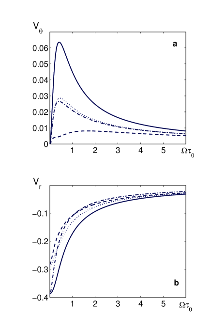
Figure 6: The effective drift velocities: (a). $V_{\theta}^{(1)}$ for $\phi_{l}=45^{\circ}$; (b). $V_{r}^{(1)}$ for $\phi_{l}=90^{\circ}$ as the functions of the parameter $\Omega\tau_{{}_{0}}$ for different values of the degrees of anisotropy: $\varepsilon=13$ and $\sigma=-2.2$ (solid); $\varepsilon=1.2$ and $\sigma=2$ (dashed); $\varepsilon=13$ and $\sigma=0$ (dotted); $\varepsilon=0$ and $\sigma=1$ (dashed).

The effective drift velocity ${\bf V}^{(2)}$ causes an additional differential rotation. Indeed, let us introduce the angular velocity difference, $\delta\Omega,$ which is determined from the identity: ${\bf V}^{(2)}=\delta\Omega\,r\,(\mbox{\boldmath$\hat{\omega}$}{\bf\times}{\bf e}).$ Comparison of this definition with Eqs. (28) and (30) yields equations for $\delta\Omega(r)\propto r^{-1}.$ Calculating the $r$-derivatives of $\delta\Omega(r)$ we obtain equations which determine the differential rotation for a slow rotation $(\omega\ll 1)$

$${\partial(\delta\Omega)\over\partial r}\approx-{4\over 5}\biggl{(}{l_{0}^{2}\Omega\over L_{\rho}\,r^{2}}\biggr{)}\biggl{(}1-{\sigma\over 6}+{5(1-\varepsilon)\over 9(\varepsilon+2)}\biggr{)}\;,$$ (32)

and for $\omega\gg 1$:

$${\partial(\delta\Omega)\over\partial r}\approx{1\over 2\omega}\biggl{(}{l_{0}u_{0}\over L_{\rho}\,r^{2}}\biggr{)}(1-\sigma)\sin^{2}\phi_{l}\;.$$ (33)

The electromotive force has a term $a_{ij}^{(c)}B_{j}$ which for an axisymmetric case contributes only to an additional effective drift velocity, ${\bf V}^{(3)},$ of the mean magnetic field, i.e.,

$$a_{ij}^{(c)}B_{j}=[{\bf V}^{(3)}{\bf\times}({\bf B}_{p}-{\bf B}_{T})]_{i}\;$$ (34)

(for details, see Appendix A), where ${\bf B}={\bf B}_{T}+{\bf B}_{p}$ is the mean magnetic field with the toroidal, ${\bf B}_{T},$ and the poloidal, ${\bf B}_{p},$ components, the tensor $a_{ij}^{(c)}$ is determined by Eq. (102), and the additional effective drift velocity is given by

$${\bf V}^{(3)} = {1\over 24}\biggl{(}{l_{0}u_{0}\over L_{\rho}}\biggr{)}\{{\bf e}[E_{7}(\omega)+E_{8}(\omega)\sin^{2}\phi_{l}$$ (35)

$$+E_{9}(\omega)\sin^{4}\phi_{l}]+{1\over 2}{\bf e}_{\theta}[E_{10}(\omega)$$

$$-E_{9}(\omega)\sin^{2}\phi_{l}]\sin(2\phi_{l})\}$$

(for details, see Appendix A). Note that for a slow rotation $(\omega\ll 1)$ the additional effective drift velocity is very small, i.e., $V^{(3)}\sim O(\omega^{2}),$ and for $\omega\gg 1$ it is given by

$${\bf V}^{(3)} \approx {\pi\over 8\omega}\biggl{(}{l_{0}u_{0}\over L_{\rho}}\biggr{)}\cos\phi_{l}\,\{{\bf e}\,\cos\phi_{l}[\lambda+10-13\sigma$$ (36)

$$-18(\sigma-1)\sin^{2}\phi_{l}]+{\bf e}_{\theta}\,\sin\phi_{l}[\lambda-\sigma$$

$$-18(\sigma-1)\cos^{2}\phi_{l}]\}\;.$$

Now we determine the total effective drift velocity in an axisymmetric case:

$$[{\bf V}^{(d)}{\bf\times}{\bf B}]_{i}+a_{ij}^{(c)}B_{j}=[{\bf V}^{(B)}{\bf\times}{\bf B}_{T}+{\bf V}^{(A)}{\bf\times}{\bf B}_{p}]_{i}\;,$$ (37)

where

$${\bf V}^{(B)}={\bf V}^{(d)}-{\bf V}^{(3)}\;,\quad{\bf V}^{(A)}={\bf V}^{(d)}+{\bf V}^{(3)}\;.$$ (38)

Therefore, the effective drift velocities, ${\bf V}^{(B)}$ and ${\bf V}^{(A)},$ for the toroidal and poloidal magnetic fields are different. The additional effective drift velocity, ${\bf V}^{(3)},$ is a result of an interaction of turbulent convection with inertial waves and Rossby waves. Indeed, a part of the tensor $a_{ij}^{(c)}({\bf k})\propto\psi_{{}_{\Omega}}\psi_{{}_{R}},$ where $\psi_{{}_{\Omega}}=2({\bf\Omega}\cdot{\bf k})/k$ is the frequency of the inertial waves and $\psi_{{}_{R}}=2\Lambda\Omega_{x}k_{y}/k^{2}$ is the frequency of Rossby waves [see Eqs. (34) and (80)].

IV Discussion

In this paper we studied an effect of rotation on a developed turbulent stratified convection. This allowed us to determine the dependencies of the hydrodynamic helicity, the alpha-tensor and the effective drift velocity of the mean magnetic field on the rate of rotation and an anisotropy of turbulence. We demonstrated that in a turbulent convection the alpha-effect can change its sign depending on the rate of rotation and an anisotropy of turbulence. We found different properties of the effective drift velocity of the mean magnetic field in a rotating turbulent convection. In particular, a poloidal effective drift velocity can be diamagnetic or paramagnetic depending on the rate of rotation. There is a difference in the effective drift velocities for the toroidal and poloidal magnetic fields which increases with the rate of rotation. We found also a toroidal effective drift velocity which can play a role of an additional differential rotation.

Some of the results obtained in our paper using the $\tau$-approximation are observed in the direct numerical simulations of the stratified turbulent convection (see OSB02 ). In particular, it was found in OSB02 that the alpha-effect can change its sign depending on the rate of rotation. It was also demonstrated in OSB02 that there is a difference in the effective drift velocities for the toroidal and poloidal magnetic fields, and that an observed toroidal effective drift velocity in OSB02 can play a role of an additional differential rotation.

Now we apply the obtained results for the analysis of an axisymmetric $\alpha\Omega$-dynamo. The mean magnetic field in an axisymmetric case is given by ${\bf B}=B{\bf e}_{\varphi}+\mbox{\boldmath$\nabla$}{\bf\times}(A{\bf e}_{\varphi}),$ where $A$ is the vector potential. The equations for $B$ and $A$ in dimensionless form are given by

$${\partial B\over\partial t}+r_{\perp}\,\mbox{\boldmath$\nabla$}{\bf\cdot}({\bf V}^{(B)}\,r_{\perp}^{-1}\,B) = D\,(\hat{\Omega}A)+\Delta_{s}B\;,$$ (39)

$${\partial A\over\partial t}+r_{\perp}^{-1}\,({\bf V}^{(A)}{\bf\cdot}\mbox{\boldmath$\nabla$})\,(r_{\perp}\,A) = \alpha B+\Delta_{s}A\;,$$ (40)

where the length is measured in units of the thickness of the convective zone $L_{c},$ the time is measured in units of $L_{c}^{2}/\eta_{{}_{T}},$ the velocity is measured in units of $\eta_{{}_{T}}/L_{c},$ the turbulent magnetic diffusion $\eta_{{}_{T}}=l_{0}u_{0}/3,$ and $u_{0}$ is the characteristic turbulent velocity in the scale $l_{0},$ $\,D=R_{\alpha}R_{\omega}$ is the dynamo number, $R_{\alpha}=L_{c}\alpha_{\ast}/\eta_{{}_{T}}$ and $R_{\omega}=L_{c}^{2}(\delta\Omega)_{\ast}/\eta_{{}_{T}}.$ Here $\alpha$ is measured in units of the maximum value $\alpha_{\ast}$ of the $\alpha$ effect, $(\delta\Omega)_{\ast}$ is the characteristic differential rotation in the scale $L_{c},$ $\hat{\Omega}A=[\mbox{\boldmath$\nabla$}(\delta\Omega){\bf\times}\mbox{\boldmath$\nabla$}(r_{\perp}\,A)]\cdot{\bf e}_{\varphi},$ $\,\Delta_{s}=\Delta-r_{\perp}^{-2},$ $r_{\perp}=r\sin\theta$ and we used the induction equation for the mean magnetic field (see, e.g., M78 ; P79 ; KR80 ; ZRS83 ; RSS88 ) and Eqs. (37) and (38). When ${\bf V}^{(A)}={\bf V}^{(B)}$ and $\mbox{\boldmath$\nabla$}{\bf\cdot}{\bf V}^{(B)}=0,$ Eqs. (39) and (40) coincide with that given in M78 . Now we seek for a solution of Eqs. (39) and (40) in the form $A,B\propto\exp(\hat{\gamma}t+i{\bf k}{\bf\cdot}{\bf x}),$ where ${\bf k}=k{\bf e}_{k},$ $\,{\bf e}_{k}={\bf e}_{\varphi}{\bf\times}{\bf e}_{{}_{\Omega}},$ the unit vector ${\bf e}_{{}_{\Omega}}$ is directed opposite to $\mbox{\boldmath$\nabla$}(\delta\Omega)$ and

$$\hat{\gamma} = \kappa/2-k^{2}-ikU^{(1)}$$ (41)

$$\pm[(\kappa/2+ikU^{(3)})^{2}+ikD]^{1/2}\;,$$

$\kappa=-\mbox{\boldmath$\nabla$}{\bf\cdot}{\bf V}^{(B)},$ $\,U^{(1,3)}={\bf V}^{(1,3)}\,{\bf\cdot}\,{\bf e}_{k}$ and $\hat{\gamma}=\gamma_{{}_{B}}+i\omega_{{}_{B}}.$ In the limit of large dynamo number $|D|$ the maximum growth rate of the mean magnetic field $\gamma_{{}_{B}}$ is given by

$$\gamma_{{}_{B}}=(3/4)(|D|/4)^{2/3}+\kappa/2\;,$$ (42)

which is achieved at the wave number $k_{m}=(1/2)(|D|/4)^{1/3}.$ At this wave number the frequency $\omega_{{}_{B}}$ of the dynamo wave is

$$\omega_{{}_{B}}=-(|D|/4)^{2/3}-(1/2)U^{(1)}(|D|/4)^{1/3}\;$$ (43)

(see KRS01 ). The negative sign of $\omega_{{}_{B}}$ implies that the dynamo waves propagate to the equator in agreement with the solar magnetic field observations. On the other hand, the divergence of the effective drift velocity ${\bf V}^{(B)}$ of the toroidal magnetic field can cause an increase of the growth rate of the mean magnetic field when $\kappa>0.$ The change of the sign of the $\alpha$-effect depending on the rate of rotation and anisotropy of turbulent convection (see Section III-B) can explain the observed direction of propagation of the solar dynamo waves.

Note that a meridional circulation in the solar convective zone can also cause an equatorward drift of the solar dynamo wave (see, e.g., M78 ; DC94 ; CSD95 ). However, it was shown recently in DBE02 that the meridional velocity, which is required for the equatorward propagation of the solar dynamo wave with the period $\sim 22$ years, should be of the order of $\sim 10-12$ m/s. Such large meridional velocities are not observed on the solar surface. On the other hand, we found that the effective drift velocities of the mean magnetic field have a meridional component (along ${\bf e}_{\theta})$. This velocity has the maximum $(V_{\theta}^{(1)})_{\rm max}\sim 10-12$ m/s in the upper part of the solar convective zone. Therefore, this meridional effective drift velocity of the mean magnetic field can cause the equatorward propagation of the solar dynamo wave in the upper part of the solar convective zone. Note that the meridional circulations in the solar convection zone and the meridional component of the effective drift velocities of the mean magnetic field are different characteristics, because the first velocity describes large-scale fluid motions (which may cause advection of the mean magnetic field by the large-scale fluid motions, i.e., by the mean flow), and the second velocity determines the drift velocity of the mean magnetic field (which is originated from the mean electromotive force $\mbox{\boldmath$\cal E$}=\langle{\bf u}\times{\bf b}\rangle).$

We found also that in the upper part of the solar convective zone the $\alpha$ effect does not change its sign, i.e., it is positive. But in the lower part of the solar convective zone the $\alpha$ effect changes its sign, because the parameter $\Omega\tau_{{}_{0}}$ increases with the increase of the depth the solar convective zone, and the $\alpha$ effect becomes negative. Therefore, in the lower part of the solar convective zone the negative $\alpha$ effect is responsible for the equatorward propagation of the solar dynamo waves. On the other hand, the meridional effective drift velocity of the mean magnetic field in the lower part of the solar convective zone is very small and, thus, it cannot be used for the explanation of the equatorward propagation of the solar dynamo wave.

Therefore, both effects, the meridional effective drift velocity of the mean magnetic field in the upper part of the solar convective zone and the sign reversal of the $\alpha$ effect in the lower part of the solar convective zone, can cause the equatorward propagation of the solar dynamo wave.

Note that in the present study we did not discuss the magnetic buoyancy effects which play an important role in a creation of strongly inhomogeneous magnetic structures (see, e.g., P79 ; KMR96 ; KR94 ; MFS92 ; FSS94 ).

Appendix A Derivations of Eqs. (17), (22), (25), (26) and (35).

A.1 The conservation equations

Equations (2) and (3) yield the following conservation equations for the kinetic energy $W_{u}=\rho_{{}_{0}}{\bf u}^{2}/2$ and for $W_{S}=\rho_{{}_{0}}S^{2}/2:$

$$\partial W_{u}/\partial t+\mbox{\boldmath$\nabla$}\cdot{\bf F}_{u} = I_{u}-D_{u}\;,$$ (44)

$$\partial W_{S}/\partial t+\mbox{\boldmath$\nabla$}\cdot{\bf F}_{S} = I_{S}-D_{S}\;,$$ (45)

where the source terms in these equations are $I_{u}=-\rho_{{}_{0}}({\bf u}\cdot{\bf g})S$ and $I_{S}=-I_{u}\tilde{\Omega}_{b}^{2}/g^{2},$ the dissipative terms are $D_{u}=-\rho_{{}_{0}}({\bf u}\cdot{\bf f}_{\nu})$ and $\,D_{S}=\rho_{{}_{0}}S\,\mbox{\boldmath$\nabla$}\cdot{\bf F}_{\kappa},$ the fluxes are ${\bf F}_{u}={\bf u}\,(W_{u}+P)$ and ${\bf F}_{S}={\bf u}W_{S}.$ Equations (44) and (45) yield a conservation equation for $W_{E}=W_{u}\tilde{\Omega}_{b}^{2}/g^{2}+W_{S}$

$$\partial W_{E}/\partial t+\mbox{\boldmath$\nabla$}\cdot{\bf F}_{E} = -D_{E}\;,$$ (46)

where the dissipative term is $D_{E}=D_{u}\tilde{\Omega}_{b}^{2}/g^{2}+D_{S}$ and the flux is ${\bf F}_{E}={\bf F}_{u}\tilde{\Omega}_{b}^{2}/g^{2}+{\bf F}_{S}.$ Equation (46) does not have a source term and it implies that without the dissipation $(D_{E}=0)$ the value $\int W_{E}\,dV$ is conserved, where in the latter formula the integration over the volume is performed. For the convection $\tilde{\Omega}_{b}^{2}<0$ and, therefore, $W_{S}\approx W_{u}|\tilde{\Omega}_{b}^{2}|/g^{2}.$ Averaging Eq. (44) over an ensemble of fluctuations we obtain a relationship between the flux of the entropy and the dissipation of the kinetic energy in a stationary turbulent convection: $\langle u_{i}S\rangle g_{i}=\langle{\bf u}\cdot{\bf f}_{\nu}\rangle.$ Similarly, averaging Eq. (46) over an ensemble of fluctuations we obtain $\langle{\bf u}^{2}\rangle=\langle S^{2}\rangle(g^{2}/|\tilde{\Omega}_{b}^{2}|).$ Equation (44) yields the relationship between $\Phi^{\ast}_{z}$ and $f_{\ast}$: $\,f_{\ast}=2\lambda g\tau_{{}_{0}}\Phi^{\ast}_{z}/\varepsilon.$

A.2 Modification of turbulent convection by rotation

Now we study a modification of turbulent convection by rotation. To this end we derive equations for the following second moments:

$$f_{ij}({\bf k}) = \hat{L}(v_{i},v_{j})\;,\quad\chi({\bf k})=\hat{L}(w,v_{z})\;,$$

$$F({\bf k}) = \hat{L}(s,w)\;,\quad G({\bf k})=\hat{L}(w,w)\;,$$

$$\Phi_{i}({\bf k}) = \hat{L}(s,v_{i})\;,\quad\Theta({\bf k})=\hat{L}(s,s)\;,$$

using Eqs. (5)-(7), where $\hat{L}(a,b)=\langle a({\bf k})b(-{\bf k})\rangle$ and ${\bf v}=\sqrt{\rho_{0}(z)}\,{\bf u}.$ The equations for these correlation functions are given by

$${\partial f({\bf k})\over\partial t} = {2\psi_{{}_{\Lambda}}\over k^{2}}\chi_{{}_{R}}({\bf k})-{2\psi_{{}_{\Omega}}\over k}\chi_{{}_{I}}({\bf k})$$ (47)

$$+2g_{\perp}({\bf k})\Phi_{R}({\bf k})+f_{{}_{N}}\;,$$

$${\partial\chi({\bf k})\over\partial t} = (ik\psi_{{}_{\Omega}}-\psi_{{}_{\Lambda}})\biggl{(}f({\bf k})-{1\over k^{2}}G({\bf k})\biggr{)}$$ (48)

$$-i\psi_{{}_{R}}\chi({\bf k})+g_{\perp}({\bf k})F(-{\bf k})+\chi_{{}_{N}}\;,$$

$${\partial\Phi_{z}({\bf k})\over\partial t} = -{\Omega_{b}^{2}\over g}f({\bf k})-{1\over k^{2}}(ik\psi_{{}_{\Omega}}-\psi_{{}_{\Lambda}})F({\bf k})$$ (49)

$$-i\psi_{{}_{R}}\Phi_{z}({\bf k})+g_{\perp}({\bf k})\Theta({\bf k})+\Phi_{N}\;,$$

$${\partial F({\bf k})\over\partial t} = -{\Omega_{b}^{2}\over g}\chi(-{\bf k})-(ik\psi_{{}_{\Omega}}+\psi_{{}_{\Lambda}})\Phi_{z}({\bf k})$$ (50)

$$+F_{N}\;,$$

$${\partial G({\bf k})\over\partial t} = 2k\psi_{{}_{\Omega}}\chi_{{}_{I}}({\bf k})-2\psi_{{}_{\Lambda}}\chi_{{}_{R}}({\bf k})+G_{N}\;,$$ (51)

$${\partial\Theta({\bf k})\over\partial t} = -2{\Omega_{b}^{2}\over g}\Phi_{R}({\bf k})+\Theta_{N}\;,$$ (52)

where

$$\Phi_{R}({\bf k}) = [\Phi_{z}({\bf k})+\Phi_{z}(-{\bf k})]/2\;,$$

$$\Phi_{I}({\bf k}) = [\Phi_{z}({\bf k})-\Phi_{z}(-{\bf k})]/2i\;,$$

and similarly for other second moments, $f_{{}_{N}},$ $\chi_{{}_{N}},\ldots,$ $\Theta_{N}$ are the third moments which are given by

$$f_{{}_{N}}({\bf k}) = \hat{L}(V_{N},v_{z})+\hat{L}(v_{z},V_{N})\;,$$

$$\chi_{{}_{N}}({\bf k}) = \hat{L}(W_{N},v_{z})+\hat{L}(w,V_{N})\;,$$

$$\Phi_{N}({\bf k}) = \hat{L}(S_{N},v_{z})+\hat{L}(s,V_{N})\;,$$

$$F_{N}({\bf k}) = \hat{L}(S_{N},w)+\hat{L}(s,W_{N})\;,$$

$$G_{N}({\bf k}) = \hat{L}(W_{N},w)+\hat{L}(w,W_{N})\;,$$

$$\Theta_{N}({\bf k}) = \hat{L}(S_{N},s)+\hat{L}(s,S_{N})\;,$$

and

$$V_{N} = -\sqrt{\rho_{0}}\,{\bf e}\cdot\{\mbox{\boldmath$\nabla$}{\bf\times}[\mbox{\boldmath$\nabla$}{\bf\times}(({\bf u}\cdot\mbox{\boldmath$\nabla$}){\bf u}-{\bf f}_{\nu})]\},$$ (53)

$$W_{N} = \sqrt{\rho_{0}}\,{\bf e}\cdot[\mbox{\boldmath$\nabla$}{\bf\times}({\bf u}{\bf\times}{\bf w}+{\bf f}_{\nu})]\;,$$ (54)

$$S_{N} = -\sqrt{\rho_{0}}\,\biggl{\{}({\bf u}\cdot\mbox{\boldmath$\nabla$})\biggl{(}{s\over\sqrt{\rho_{0}}}\biggr{)}$$ (55)

$$+{1\over T_{0}}\,{\rm div}\,\biggl{[}{\bf F}_{\kappa}\biggl{(}{s\over\sqrt{\rho_{0}}}\biggr{)}\biggr{]}\biggr{\}}\;,$$

$\psi_{{}_{\Lambda}}={\bf\Omega}\cdot{\bf\Lambda},$ $\quad\psi_{{}_{\Omega}}=2({\bf\Omega}\cdot{\bf k})/k,$ $\quad\psi_{{}_{R}}=2\Lambda\Omega_{x}k_{y}/k^{2},$ and $g_{\perp}({\bf k})=g(k_{\perp}/k)^{2}.$ We assumed that $(1/4)\Lambda^{2}\ll k^{2}.$ Now we introduce the following variables:

$$\chi_{p}({\bf k}) = k\psi_{{}_{\Omega}}\,\chi_{{}_{R}}({\bf k})+\psi_{{}_{\Lambda}}\,\chi_{{}_{I}}({\bf k})\;,$$

$$\chi_{m}({\bf k}) = k\psi_{{}_{\Omega}}\,\chi_{{}_{I}}({\bf k})-\psi_{{}_{\Lambda}}\,\chi_{{}_{R}}({\bf k})\;,$$

$$F_{p}({\bf k}) = k\psi_{{}_{\Omega}}\,F_{R}({\bf k})-\psi_{{}_{\Lambda}}\,F_{I}({\bf k})\;,$$

$$F_{m}({\bf k}) = k\psi_{{}_{\Omega}}\,F_{I}({\bf k})+\psi_{{}_{\Lambda}}\,F_{R}({\bf k})\;,$$

which allow us to rewrite Eqs. (47)-(52) as follows

$${\partial f({\bf k})\over\partial t} = -{2\over k^{2}}\chi_{m}({\bf k})+2g_{\perp}({\bf k})\Phi_{R}({\bf k})$$ (56)

$$+f_{{}_{N}}\;,$$

$${\partial\chi_{p}({\bf k})\over\partial t} = \psi_{{}_{R}}\chi_{m}({\bf k})+g_{\perp}({\bf k})F_{p}({\bf k})+\chi_{{}_{N}}^{(p)}\;,$$ (57)

$${\partial\chi_{m}({\bf k})\over\partial t} = (k\psi_{{}_{\Omega}})^{2}\biggl{(}f({\bf k})-{1\over k^{2}}G({\bf k})\biggr{)}-\psi_{{}_{R}}\chi_{p}({\bf k})$$ (58)

$$-g_{\perp}({\bf k})F_{m}({\bf k})+\chi_{{}_{N}}^{(m)}\;,$$

$${\partial\Phi_{R}({\bf k})\over\partial t} = {1\over k^{2}}F_{m}({\bf k})+\psi_{{}_{R}}\Phi_{I}({\bf k})$$ (59)

$$+g_{\perp}({\bf k})\Theta({\bf k})+\Phi_{N}^{(R)}\;,$$

$${\partial\Phi_{I}({\bf k})\over\partial t} = -{1\over k^{2}}F_{p}({\bf k})-\psi_{{}_{R}}\Phi_{R}({\bf k})+\Phi_{N}^{(I)}\;,$$ (60)

$${\partial F_{p}({\bf k})\over\partial t} = (k\psi_{{}_{\Omega}})^{2}\Phi_{I}({\bf k})+F_{N}^{(p)}\;,$$ (61)

$${\partial F_{m}({\bf k})\over\partial t} = -(k\psi_{{}_{\Omega}})^{2}\Phi_{R}({\bf k})+F_{N}^{(m)}\;,$$ (62)

$${\partial G({\bf k})\over\partial t} = {2\over k^{2}}\chi_{m}({\bf k})+G_{N}\;,$$ (63)

$${\partial\Theta({\bf k})\over\partial t} = \Theta_{N}\;,$$ (64)

where we neglected small terms proportional to $\Omega_{b}^{2}/g.$

Next, we use the $\tau$-approximation which allows us to express the third moments $f_{{}_{N}},$ $\chi_{{}_{N}}^{(p)},\ldots,$ $\Theta_{N}$ in Eqs. (56)-(64) in terms of the second moments [see Eqs. (8)], where the superscript $(0)$ corresponds to the background turbulent convection (it is a turbulent convection without rotation, ${\bf\Omega}=0),$ and $\tau(k)$ is the characteristic relaxation time of the statistical moments. We consider the background turbulent convection with $\chi^{(0)}({\bf k})=0.$

We assume that the characteristic times of variation of the second moments $f({\bf k}),$ $\chi_{p}({\bf k}),\ldots,$ $\Theta({\bf k})$ are substantially larger than the correlation time $\tau(k)$ for all turbulence scales. This allows us to get a stationary solution of Eqs. (56)-(64):

$$f({\bf k}) = f^{(0)}({\bf k})-2\psi_{{}_{\Omega}}^{2}[\mu_{1}({\bf k})$$ (65)

$$+\tau(k)g_{\perp}({\bf k})\Phi_{R}({\bf k})]\;,$$

$$\chi_{{}_{R}}({\bf k}) = -\psi_{{}_{\Lambda}}\mu_{1}({\bf k})+k\psi_{{}_{\Omega}}\psi_{{}_{R}}\mu_{2}({\bf k})\;,$$ (66)

$$\chi_{{}_{I}}({\bf k}) = k\psi_{{}_{\Omega}}\mu_{1}({\bf k})\;,$$ (67)

$$\Phi_{R}({\bf k}) = {\Phi^{(0)}({\bf k})\over 1+\psi_{{}_{\Omega}}^{2}}\;,$$ (68)

$$\Phi_{I}({\bf k}) = -{\psi_{{}_{R}}\Phi^{(0)}({\bf k})\over(1+\psi_{{}_{\Omega}}^{2})^{2}}\;,$$ (69)

$$F_{R}({\bf k}) = k\psi_{{}_{\Omega}}\Phi_{I}({\bf k})-\psi_{{}_{\Lambda}}\Phi_{R}({\bf k})\;,$$ (70)

$$F_{I}({\bf k}) = F_{I}^{(0)}({\bf k})-k\psi_{{}_{\Omega}}\Phi_{R}({\bf k})\;,$$ (71)

$$G({\bf k}) = G^{(0)}({\bf k})+2(k\psi_{{}_{\Omega}})^{2}\mu_{1}({\bf k})\;,$$ (72)

$$\Theta({\bf k}) = \Theta^{(0)}({\bf k})\;,$$ (73)

where we changed $\tau\psi_{{}_{R}}\to\psi_{{}_{R}},$ $\quad\tau\psi_{{}_{\Omega}}\to\psi_{{}_{\Omega}},$ $\quad\tau\psi_{{}_{\Lambda}}\to\psi_{{}_{\Lambda}},$

$$\mu_{1}({\bf k}) = -{1\over 1+4\psi_{{}_{\Omega}}^{2}}[\varepsilon f^{(0)}({\bf k})$$

$$-\tau(k)g_{\perp}({\bf k})\Phi_{R}({\bf k})(1-2\psi_{{}_{\Omega}}^{2})]\;,$$

$$\mu_{2}({\bf k}) = \mu_{1}({\bf k})-{\tau(k)g_{\perp}({\bf k})\Phi_{R}({\bf k})\over 1+\psi_{{}_{\Omega}}^{2}}\;,$$

and $f^{(0)}({\bf k})-G^{(0)}({\bf k})/k^{2}\equiv-\varepsilon f^{(0)}({\bf k}).$ Here we neglected the terms $\sim O[(\Lambda l_{0})^{2}].$ We will show below that the first term in Eq. (66), $\chi_{{}_{R}}^{(1)}({\bf k})=-\psi_{{}_{\Lambda}}\mu_{1}({\bf k}),$ contributes to the $\alpha$-effect, whereas the second term in Eq. (66), $\chi_{{}_{R}}^{(2)}({\bf k})=k\psi_{{}_{\Omega}}\psi_{{}_{R}}\mu_{2}({\bf k}),$ contributes to the additional effective drift velocity. Thus, Eqs. (65)-(73) describe a modification of turbulent convection by rotation.

A.3 The correlation tensor of velocity field

The functions $f({\bf k}),$ $G({\bf k})$ and $\chi({\bf k})$ determine the correlation tensor $f_{ij}({\bf k})\equiv\langle v_{i}({\bf k})v_{j}(-{\bf k})\rangle$:

$$f_{ij}({\bf k}) = f_{ij}^{(a)}({\bf k})+f_{ij}^{(b)}({\bf k})\;,$$ (74)

$$f_{ij}^{(a)}({\bf k}) = \biggl{(}{k_{\perp}\over k}\biggr{)}^{2}\biggl{\{}f({\bf k})P_{ij}(k)$$ (75)

$$-\biggl{(}f({\bf k})-{1\over k^{2}}G({\bf k})\biggr{)}P_{ij}^{(\perp)}(k_{\perp})$$

$$+(i/2k^{2})(k_{j}\Lambda_{i}-k_{i}\Lambda_{j})f({\bf k})\biggr{\}}\;,$$

$$f_{ij}^{(b)}({\bf k}) = (1/2k_{\perp}^{4})\{[i({\bf k}\cdot{\bf e})B_{ij}^{(M)}-(\Lambda/2)B_{ij}^{(P)}$$ (76)

$$-i2k_{\perp}^{2}\varepsilon_{ijp}k_{p}]\chi_{{}_{R}}({\bf k})+[({\bf k}\cdot{\bf e})B_{ij}^{(P)}$$

$$-(i\Lambda/2)B_{ij}^{(M)}-2k_{\perp}^{2}A_{ij}^{(P)}]\chi_{{}_{I}}({\bf k})\}\;,$$

and $P_{ij}(k)=\delta_{ij}-k_{ij},$ $\quad k_{ij}=k_{i}k_{j}/k^{2},$ $\quad{\bf k}={\bf k}_{\perp}+({\bf k}\cdot{\bf e}){\bf e},$ $\quad P_{ij}^{(\perp)}(k_{\perp})=\delta_{ij}-k^{\perp}_{ij}-e_{ij},$ $\quad k^{\perp}_{ij}=({\bf k}_{\perp})_{i}({\bf k}_{\perp})_{j}/k_{\perp}^{2},$ $\quad e_{ij}=e_{i}e_{j},$ and $A_{ij}^{(P)}=({\bf k}_{\perp}{\bf\times}{\bf e})_{i}e_{j}+({\bf k}_{\perp}{\bf\times}{\bf e})_{j}e_{i},$ $B_{ij}^{(P)}=({\bf k}_{\perp}{\bf\times}{\bf e})_{i}({\bf k}_{\perp})_{j}+({\bf k}_{\perp}{\bf\times}{\bf e})_{j}({\bf k}_{\perp})_{i}$ and $B_{ij}^{(M)}=({\bf k}_{\perp}{\bf\times}{\bf e})_{i}({\bf k}_{\perp})_{j}-({\bf k}_{\perp}{\bf\times}{\bf e})_{j}({\bf k}_{\perp})_{i}.$ For the derivation of Eqs. (75) and (76) the velocity ${\bf v}_{\perp}$ is written as a sum of the vortical and the potential components, i.e., ${\bf v}_{\perp}=\mbox{\boldmath$\nabla$}{\bf\times}(C{\bf e})+\mbox{\boldmath$\nabla$}_{\perp}\tilde{\varphi},$ where ${\bf v}={\bf v}_{\perp}+v_{z}{\bf e},$ $\quad w=-\Delta_{\perp}C,$ $\quad\Delta_{\perp}\tilde{\varphi}=\Lambda v_{z}/2-\partial v_{z}/\partial z,$ $\quad\mbox{\boldmath$\nabla$}\cdot{\bf v}=(\Lambda/2)({\bf v}\cdot{\bf e}),$ $\quad\mbox{\boldmath$\nabla$}_{\perp}=\mbox{\boldmath$\nabla$}-{\bf e}({\bf e}\cdot\mbox{\boldmath$\nabla$}).$ We also used the identities $({\bf k}_{\perp}{\bf\times}{\bf e})_{i}({\bf k}_{\perp}{\bf\times}{\bf e})_{j}=k_{\perp}^{2}P_{ij}^{(\perp)}(k_{\perp})$ and $({\bf k}\cdot{\bf e})B_{ij}^{(M)}-k_{\perp}^{2}A_{ij}^{(M)}=k_{\perp}^{2}\varepsilon_{ijp}k_{p}$ (see, e.g., EKR98 ). In Eq. (76) we neglected the terms $\sim O[(\Lambda l_{0})^{2}].$ We will use Eqs. (75) and (76) for the calculation of the hydrodynamic helicity and the $\alpha$ effect.

A.4 The hydrodynamic helicity

Now we find the dependence of the hydrodynamic helicity $\chi^{(v)}=\langle{\bf u}\cdot(\mbox{\boldmath$\nabla$}{\bf\times}{\bf u})\rangle$ on the rate of rotation and anisotropy of turbulence. In ${\bf k}$-space the hydrodynamic helicity is given by

$$\chi^{(v)}({\bf k}) \equiv -i\,\varepsilon_{inm}k_{i}f_{mn}({\bf k})\exp(\Lambda z)$$ (77)

$$= (1+k^{2}/k_{\perp}^{2})\chi_{{}_{R}}({\bf k})\exp(\Lambda z)\;,$$

where we used Eqs. (75) and (76). The function $\exp(\Lambda z)$ in Eq. (77) implies that we used the transformation ${\bf u}=\exp(\Lambda z/2){\bf v}.$ Equation (77) can be rewritten as

$$\chi^{(v)}({\bf k})=\exp(\Lambda z)[\chi_{1}({\bf k})+\chi_{2}({\bf k})]\;,$$ (78)

where

$$\chi_{1}({\bf k}) = -\psi_{{}_{\Lambda}}\mu_{1}({\bf k})(1+k^{2}/k_{\perp}^{2})\;,$$ (79)

$$\chi_{2}({\bf k}) = -4\tau^{2}\Omega^{2}\Lambda(\mbox{\boldmath$\hat{\omega}$}\times{\bf e})_{m}\hat{\omega}_{n}k_{mn}\mu_{2}({\bf k})(1$$ (80)

$$+k^{2}/k_{\perp}^{2})\;,$$

where $\mbox{\boldmath$\hat{\omega}$}={\bf\Omega}/\Omega$ and we used the identity $k\psi_{{}_{\Omega}}\psi_{{}_{R}}=-4\tau^{2}\Omega^{2}\Lambda(\mbox{\boldmath$\hat{\omega}$}\times{\bf e})_{m}\hat{\omega}_{n}k_{mn}.$ The integration in ${\bf k}$-space in $\chi_{1,2}=\int\chi_{1,2}({\bf k})\,d{\bf k}$ yields

$$\chi_{1} = -{1\over 12\delta_{\ast}}\biggl{(}{l_{0}^{2}\Omega\over L_{\rho}\tau_{{}_{0}}}\biggr{)}\sin\phi_{l}\,\{(\sigma+3)\phi_{{}_{1}}\{I_{mm}^{(2)}\}$$ (81)

$$+(7\sigma-9)\phi_{{}_{1}}\{M_{mm}^{(2)}\}-3(\sigma-1)\phi_{{}_{1}}\{e_{mn}M_{mn}^{(2)}\}$$

$$+(\lambda/2)[M_{mm}^{(1)}(2\omega)-2I_{mm}^{(1)}(2\omega)]\}\;,$$

$$\chi_{2} \propto (\mbox{\boldmath$\hat{\omega}$}\times{\bf e})_{m}\hat{\omega}_{n}[I_{mn}^{(p)}(\omega)-M_{mn}^{(p)}(\omega)]=0\;,$$ (82)

where $\omega=4\tau_{{}_{0}}\Omega,$ $\,u_{0}^{2}=2g\tau_{{}_{0}}\Phi^{\ast}_{z}\delta_{\ast},$ $\,\sin\phi_{l}=\mbox{\boldmath$\hat{\omega}$}\cdot{\bf e},$ $\,l_{0}=u_{0}\tau_{{}_{0}},$ $\,\phi_{{}_{1}}\{X\}=2X(2\omega)-X(\omega),$ e.g., $\,\phi_{{}_{1}}\{I_{mn}^{(2)}\}=2I_{mn}^{(2)}(2\omega)-I_{mn}^{(2)}(\omega),$

$$I_{ij}^{(p)}(\omega) = (6/\pi\omega^{p+1})\int_{0}^{\omega}y^{p}\bar{I}_{ij}(y^{2})\,dy\;,$$ (83)

$$M_{ij}^{(p)}(\omega) = (6/\pi\omega^{p+1})\int_{0}^{\omega}y^{p}\bar{M}_{ij}(y^{2})\,dy\;,$$ (84)

$\bar{M}_{ij}(y)=e_{mn}\bar{I}_{ijmn}(y),$ $\,\bar{I}_{ij}(z)$ and $\bar{I}_{ijmn}(z)$ are determined by Eqs. (118) and (119) in Appendix B, and the exponent $p=1,2,3,4$ is determined by $\tau^{p}$ in the expressions for the the hydrodynamic helicity, the $\alpha$ effect and the effective drift velocity (see below). For example, $p=1,2$ in Eq. (81). Equation (81) yields the angular velocity dependence of the hydrodynamic helicity $\chi^{(v)}$ which is given by Eq. (17).

A.5 The electromotive force

In order to derive equation for the $\alpha$-tensor we introduce the electromotive force

$${\cal E}_{i}=\langle{\bf u}\times{\bf b}\rangle_{i}=\exp(\Lambda z)\varepsilon_{imn}\int\chi^{(c)}_{mn}({\bf k})\,d{\bf k}\;,$$ (85)

where $\chi^{(c)}_{ij}({\bf k})=\hat{L}(v_{i},h_{j})\equiv\langle v_{i}({\bf k})h_{j}(-{\bf k})\rangle$ is the cross-helicity tensor. Using equation for ${\bf v}=\mbox{\boldmath$\nabla$}{\bf\times}(C{\bf e})+\mbox{\boldmath$\nabla$}_{\perp}\tilde{\varphi}+v_{z}{\bf e}$ we obtain

$$\chi^{(c)}_{ij}({\bf k}) = k_{\perp}^{-2}\{i({\bf k}{\bf\times}{\bf e})_{i}\xi_{j}({\bf k})+[k_{\perp}^{2}e_{i}-(k_{i}$$ (86)

$$-k_{z}e_{i})(k_{z}+i\Lambda/2)]\chi^{(c)}_{j}({\bf k})\}\;,$$

where $\chi^{(c)}_{j}({\bf k})=e_{i}\chi^{(c)}_{ij}({\bf k})=\hat{L}(v_{z},h_{j})$ and $\mbox{\boldmath$\xi$}({\bf k})=\hat{L}(w,{\bf h}).$ Using Eqs. (5)-(7) and (21) we derive equations for $\mbox{\boldmath$\xi$}({\bf k}),$ $\,\mbox{\boldmath$\chi$}^{(c)}({\bf k})$ and $\mbox{\boldmath$\zeta$}({\bf k})=\hat{L}(s,{\bf h})$:

$${\partial\mbox{\boldmath$\xi$}\over\partial t} = {\bf I}^{(w)}+(ik\psi_{{}_{\Omega}}-\psi_{{}_{\Lambda}})\mbox{\boldmath$\chi$}^{(c)}({\bf k})+\mbox{\boldmath$\xi$}_{{}_{N}}\;,$$ (87)

$${\partial\mbox{\boldmath$\chi$}^{(c)}\over\partial t} = {\bf I}^{(v)}+k^{-2}(ik\psi_{{}_{\Omega}}+\psi_{{}_{\Lambda}})\mbox{\boldmath$\xi$}({\bf k})+i\psi_{{}_{R}}\mbox{\boldmath$\chi$}^{(c)}$$ (88)

$$+g_{\perp}({\bf k})\mbox{\boldmath$\zeta$}+\mbox{\boldmath$\chi$}^{(c)}_{{}_{N}}\;,$$

$${\partial\mbox{\boldmath$\zeta$}\over\partial t} = {\bf I}^{(s)}+\mbox{\boldmath$\zeta$}_{{}_{N}}\;,$$ (89)

where $\mbox{\boldmath$\xi$}_{{}_{N}},$ $\,\mbox{\boldmath$\chi$}^{(c)}_{{}_{N}}$ and $\,\mbox{\boldmath$\zeta$}_{{}_{N}}$ are the third moments:

$$\mbox{\boldmath$\xi$}_{{}_{N}}({\bf k}) = \hat{L}(W_{N},{\bf h})+\hat{L}(w,{\bf H}_{N})\;,$$

$$\mbox{\boldmath$\chi$}^{(c)}_{{}_{N}}({\bf k}) = \hat{L}(V_{N},{\bf h})+\hat{L}(v_{z},{\bf H}_{N})\;,$$

$$\mbox{\boldmath$\zeta$}_{{}_{N}}({\bf k}) = \hat{L}(S_{N},{\bf h})+\hat{L}(s,{\bf H}_{N})\;,$$

and

$${\bf H}_{N} = \sqrt{\rho_{0}}\,\,\mbox{\boldmath$\nabla$}{\bf\times}({\bf u}{\bf\times}{\bf b}-\mbox{\boldmath$\cal E$}-\eta\,\mbox{\boldmath$\nabla$}{\bf\times}{\bf b})\;,$$ (90)

$\psi_{{}_{\Lambda}}={\bf\Omega}\cdot{\bf\Lambda},$ $\quad\psi_{{}_{\Omega}}=2({\bf\Omega}\cdot{\bf k})/k,$ $\quad\psi_{{}_{R}}=2\Lambda\Omega_{x}k_{y}/k^{2},$ and

$$I_{j}^{(v)} = \hat{L}\biggl{(}v_{z},{\partial h_{j}\over\partial t}\biggr{)}=-i\,({\bf B}\cdot\tilde{\bf k})e_{i}f_{ij}({\bf k})$$ (91)

$$-\Lambda f({\bf k})\,B_{j}\;,$$

$${\bf I}^{(w)} = \hat{L}\biggl{(}w,{\partial{\bf h}\over\partial t}\biggr{)}=-i\,({\bf B}\cdot\tilde{\bf k})\,\mbox{\boldmath$\chi$}^{(w)}({\bf k})$$ (92)

$$-\Lambda\chi({\bf k})\,{\bf B}\;,$$

$${\bf I}^{(s)} = \hat{L}\biggl{(}s,{\partial{\bf h}\over\partial t}\biggr{)}=-i\,({\bf B}\cdot\tilde{\bf k})\,{\bf\Phi}({\bf k})$$ (93)

$$-\Lambda\Phi_{z}({\bf k})\,{\bf B}\;,$$

$\tilde{\bf k}={\bf k}+(i\Lambda/2){\bf e}$ and $\mbox{\boldmath$\chi$}^{(w)}({\bf k})\equiv\hat{L}(w,{\bf v})$ is given by

$$\mbox{\boldmath$\chi$}^{(w)}({\bf k}) = k_{\perp}^{-2}\{\chi({\bf k})[{\bf e}(k^{2}-i\Lambda k_{z}/2)-{\bf k}(k_{z}$$ (94)

$$-i\Lambda/2)]-iG({\bf k})({\bf k}{\bf\times}{\bf e})\}\;.$$

Note that $\chi({\bf k})=\mbox{\boldmath$\chi$}^{(w)}({\bf k})\cdot{\bf e}.$ Now we use the $\tau$-approximation and assume that the characteristic times of variation of the second moments $\mbox{\boldmath$\xi$},$  $\zeta$ and $\mbox{\boldmath$\chi$}^{(c)}$ are substantially larger than the correlation time $\tau(k)$ for all turbulence scales. This allows us to get a stationary solution of Eqs. (87)-(89):

$$\mbox{\boldmath$\xi$}({\bf k}) = \tau{\bf I}^{(w)}({\bf k})+(ik\psi_{{}_{\Omega}}-\psi_{{}_{\Lambda}})\mbox{\boldmath$\chi$}^{(c)}({\bf k})\;,$$ (95)

$$\mbox{\boldmath$\chi$}^{(c)} = {\tau(1+\psi_{{}_{\Omega}}^{2}+i\psi_{{}_{R}})\over(1+\psi_{{}_{\Omega}}^{2})^{2}}[{\bf I}^{(v)}$$ (96)

$$+k^{-2}(ik\psi_{{}_{\Omega}}+\psi_{{}_{\Lambda}}){\bf I}^{(w)}({\bf k})]\;,$$

and $\mbox{\boldmath$\zeta$}({\bf k})=\tau{\bf I}^{(s)},$ where we changed $\tau\psi_{{}_{R}}\to\psi_{{}_{R}},$ $\quad\tau\psi_{{}_{\Omega}}\to\psi_{{}_{\Omega}},$ $\quad\tau\psi_{{}_{\Lambda}}\to\psi_{{}_{\Lambda}}.$ Now we take into account that a general form of the electromotive force is given by

$${\cal E}_{i} = \alpha_{ij}B_{j}+({\bf V}^{(d)}{\bf\times}{\bf B})_{i}-\eta_{ij}(\mbox{\boldmath$\nabla$}{\bf\times}{\bf B})_{j}-\kappa_{ijk}(\partial\hat{B})_{ij}$$ (97)

$$-[\mbox{\boldmath$\delta$}{\bf\times}(\mbox{\boldmath$\nabla$}{\bf\times}{\bf B})]_{i}\equiv a_{ij}B_{j}+b_{ijk}B_{i,j}\;,$$

(see, e.g., R80 ), where the tensors $\alpha_{ij}$ and $\eta_{ij}$ describe the $\alpha$-effect and turbulent magnetic diffusion, respectively, ${\bf V}^{(d)}$ is the effective diamagnetic (or paramagnetic) velocity, $\kappa_{ijk}$ and $\delta$ describe a nontrivial behavior of the mean magnetic field in an anisotropic turbulence, $B_{i,j}=\nabla_{j}B_{i},$ $\quad(\partial\hat{B})_{ij}=(1/2)(B_{i,j}+B_{j,i}).$ In this study we determine only the tensor $\alpha_{ij}$ and the velocity $V_{k}^{(d)}.$ The calculations of the other coefficients defining electromotive force is a subject of a separate paper. The tensor $a_{ij}\equiv a_{ij}^{(S)}+a_{ij}^{(AS)}$ follows from Eqs. (86), (95)-(97), where

$$a_{ij}^{(S)} = a_{ij}^{(a)}+a_{ij}^{(b)}+a_{ij}^{(c)}\;,$$ (98)

$$a_{ij}^{(AS)} = a_{ij}^{(d)}+a_{ij}^{(e)}\;,$$ (99)

where $a_{ij}^{(S)}=(1/2)(a_{ij}+a_{ji})$ and $a_{ij}^{(AS)}=(1/2)(a_{ij}-a_{ji})$ are the symmetric and antisymmetric parts of the tensor $a_{ij},$ and

$$a_{ij}^{(a)}({\bf k}) = k_{ij}\psi_{{}_{\Lambda}}s_{1}({\bf k},z)[2\mu_{1}({\bf k})+f({\bf k})-G({\bf k})/k^{2}$$ (100)

$$+2\tau(k)g_{\perp}({\bf k})\Phi_{R}({\bf k})]\;,$$

$$a_{ij}^{(b)}({\bf k}) = (e_{i}k_{j}+e_{j}k_{i})s_{2}({\bf k},z)[\psi_{{}_{\Omega}}G({\bf k})-k\chi_{{}_{I}}({\bf k})$$ (101)

$$+k\tau(k)g_{\perp}({\bf k})F_{I}({\bf k})]\;.$$

$$a_{ij}^{(c)}({\bf k}) = \biggl{[}\biggl{(}{f({\bf k})+G({\bf k})/k^{2}+2\tau(k)g_{\perp}({\bf k})\Phi_{R}({\bf k})\over 1+\psi_{{}_{\Omega}}^{2}}$$ (102)

$$-2\mu_{2}({\bf k})\biggr{)}k\psi_{{}_{\Omega}}-\chi_{{}_{I}}({\bf k})\biggr{]}k_{ij}\psi_{{}_{R}}s_{1}({\bf k},z)$$

$$+[({\bf e}{\bf\times}{\bf k})_{i}k_{j}+({\bf e}{\bf\times}{\bf k})_{j}k_{i}]s_{2}({\bf k},z)[kf({\bf k})$$

$$+k\tau(k)g_{\perp}({\bf k})\Phi_{R}({\bf k})-\psi_{{}_{\Omega}}\chi_{{}_{I}}({\bf k})]\;,$$

$$a_{ij}^{(d)}({\bf k}) = [2k^{2}\varepsilon_{ijm}e_{n}P_{mn}(k)+({\bf e}{\bf\times}{\bf k})_{i}k_{j}$$ (103)

$$-({\bf e}{\bf\times}{\bf k})_{j}k_{i}]s_{2}({\bf k},z)[kf({\bf k})$$

$$-\psi_{{}_{\Omega}}\chi_{{}_{I}}({\bf k})+k\tau(k)g_{\perp}({\bf k})\Phi_{R}({\bf k})]\;,$$

$$a_{ij}^{(e)}({\bf k}) = k[2\varepsilon_{ijm}({\bf e}{\bf\times}{\bf k})_{m}-e_{i}k_{j}$$ (104)

$$+e_{j}k_{i}]s_{2}({\bf k},z)\{k\psi_{{}_{\Omega}}[f({\bf k})$$

$$+\tau(k)g_{\perp}({\bf k})\Phi_{R}({\bf k})]+\chi_{{}_{I}}({\bf k})\}\;,$$

and $s_{1}({\bf k},z)=\exp(\Lambda z)\tau(k)(k/k_{\perp})^{2}/(1+\psi_{{}_{\Omega}}^{2}),$ $\,s_{2}({\bf k},z)=(\Lambda/2k^{3})s_{1}({\bf k},z).$ Here we used that

$$\cal E = k_{\perp}^{-2}[i\mbox{\boldmath$\xi$}{\bf\times}({\bf e}{\bf\times}{\bf k})+({\bf e}{\bf\times}\mbox{\boldmath$\chi$}^{(c)})(k^{2}+i\Lambda k_{z}/2)$$ (105)

$$-({\bf k}{\bf\times}\mbox{\boldmath$\chi$}^{(c)})(k_{z}+i\Lambda/2)]\;,$$

$$e_{i}f_{ij}({\bf k}) = k_{\perp}^{-2}\{[k^{2}e_{i}P_{ij}({\bf k})+i(\Lambda/2)k_{i}P_{ij}({\bf e})]f({\bf k})$$ (106)

$$+i({\bf e}{\bf\times}{\bf k})_{j}[\chi_{{}_{R}}({\bf k})-i\chi_{{}_{I}}({\bf k})]\}\;,$$

where $P_{ij}({\bf e})=\delta_{ij}-e_{ij}.$ Note that $e_{i}f_{ij}({\bf k})\not=e_{i}f_{ji}({\bf k})$ because rotation causes a nonzero helicity in the turbulent convection. Here we also took into account that the tensor $a_{ij}$ must be real in ${\bf r}$-space.

We will show that the tensors $a_{ij}^{(a)}({\bf k})$ and $a_{ij}^{(b)}({\bf k})$ contribute to the $\alpha$-tensor, the tensor $a_{ij}^{(d)}({\bf k})$ contributes to the effective drift velocity ${\bf V}^{(1)},$ the tensor $a_{ij}^{(e)}({\bf k})$ contributes to the effective drift velocity ${\bf V}^{(2)},$ and the tensor $a_{ij}^{(c)}({\bf k})$ contributes to the effective drift velocity ${\bf V}^{(3)}.$

A.6 The $\alpha$-tensor

Now we determine the tensor $\alpha_{ij}=a_{ij}^{(a)}+a_{ij}^{(b)}.$ The integration in ${\bf k}$-space yields

$$a_{ij}^{(a)} = {1\over 6\delta_{\ast}}\biggl{(}{l_{0}^{2}\Omega\over L_{\rho}}\biggr{)}[\phi_{{}_{5}}\{I_{ij}\}$$ (107)

$$+3(\sigma-1)\phi_{{}_{2}}\{M_{ij}^{(3)}\}]\sin\phi_{l}\;,$$

$$a_{ij}^{(b)} = {1\over 6\delta_{\ast}}\biggl{(}{l_{0}^{2}\Omega\over L_{\rho}}\biggr{)}\hat{P}^{(b)}_{ijmn}[\phi_{{}_{6}}\{I_{mn}\}$$ (108)

$$+3(\sigma-1)\phi_{{}_{3}}\{M_{mn}^{(3)}\}]\;.$$

where Eqs. (100) and (101) for $a_{ij}^{(a)}({\bf k})$ and $a_{ij}^{(b)}({\bf k}),$ respectively, $\hat{P}^{(b)}_{ijmn}=\hat{\omega}_{m}(e_{i}\delta_{nj}+e_{j}\delta_{ni}),$ and hereafter we use the following functions:

$$\phi_{{}_{1}}\{X\} = 2X(2\omega)-X(\omega)\;,\,$$

$$\phi_{{}_{2}}\{X\} = 4X(2\omega)-{3\over\pi}\bar{X}(\omega^{2})\;,$$

$$\phi_{{}_{3}}\{X\} = {3\over\pi}\bar{X}(\omega^{2})-2X(2\omega)-X(\omega)\;,$$

$$\phi_{{}_{4}}\{X\} = 7X^{(4)}(\omega)-4X^{(4)}(2\omega)$$

$$-{3\over\pi}\bar{X}(\omega^{2})+{9\omega^{2}\over\pi}\biggl{(}{\partial\bar{X}(a)\over\partial a}\biggr{)}_{a=\omega^{2}}\;,$$

$$\phi_{{}_{5}}\{X\} = (3-\sigma)\phi_{{}_{2}}\{X^{(3)}\}-(\lambda/2)[4X^{(2)}(2\omega)$$

$$-X^{(2)}(\omega)]\;,$$

$$\phi_{{}_{6}}\{X\} = (3-\sigma)\phi_{{}_{3}}\{X^{(3)}\}+(\lambda/2)[2X^{(2)}(2\omega)$$

$$+\varepsilon^{-1}X^{(2)}(\omega)]\;,$$

$$\phi_{{}_{7}}\{X\} = (3-\sigma)\phi_{{}_{1}}\{X^{(2)}\}-\lambda[X^{(1)}(2\omega)$$

$$-(1+\varepsilon^{-1})X^{(1)}(\omega)]\;,$$

$$\phi_{{}_{8}}\{X\} = (3-\sigma)\phi_{{}_{1}}\{X^{(3)}\}-(\lambda/2)[\phi_{{}_{1}}\{X^{(2)}\}$$

$$-\varepsilon^{-1}X^{(2)}(\omega)]\;,$$

$$\phi_{{}_{9}}\{X\} = 4\lambda X^{(3)}(2\omega)-(\lambda+2\delta_{\ast})X^{(3)}(\omega)$$

$$+{6\delta_{\ast}\over\pi}\bar{X}(\omega^{2})\;.$$

For example,

$$\phi_{{}_{3}}\{M_{mn}^{(3)}\} = {3\over\pi}\bar{M}_{mn}(\omega^{2})-2M_{mn}^{(3)}(2\omega)-M_{mn}^{(3)}(\omega)\;,$$

$$\phi_{{}_{6}}\{I_{mn}\} = (3-\sigma)\phi_{{}_{3}}\{I_{mn}^{(3)}\}+(\lambda/2)[2I_{mn}^{(2)}(2\omega)$$

$$+\varepsilon^{-1}I_{mn}^{(2)}(\omega)]\;,$$

the functions $I_{mn}^{(2)}(\omega)$ and $M_{mn}^{(3)}(\omega)$ are determined by Eqs. (83) and (84), $\bar{M}_{ij}(y)=e_{mn}\bar{I}_{ijmn}(y),$ and the functions $\bar{I}_{ij}(z)$ and $\bar{I}_{ijmn}(z)$ are determined by Eqs. (118) and (119) in Appendix B. Now we use the following identities

$$\hat{P}^{(b)}_{ijmn}\bar{I}_{mn} = (e_{i}\hat{\omega}_{j}+e_{j}\hat{\omega}_{i})\bar{L}_{1}\;,$$

$$\hat{P}^{(b)}_{ijmn}\bar{M}_{mn} = (e_{i}\hat{\omega}_{j}+e_{j}\hat{\omega}_{i})(\bar{L}_{3}+\bar{L}_{2}\sin^{2}\phi_{l})$$

$$+4\,e_{ij}\,\bar{L}_{3}\,\sin\phi_{l}\,,$$

where $\bar{L}_{k}$ are determined by Eqs. (139) in Appendix C. Thus, the $\alpha$-tensor, $\alpha_{ij}\equiv a_{ij}^{(a)}+a_{ij}^{(b)},$ is given by Eq. (22). For a slow rotation $(\omega\ll 1)$ the tensor $\alpha_{ij}$ is given by

$$\alpha_{ij} \approx \alpha\delta_{ij}-{4\over 5}\biggl{(}{l_{0}^{2}\Omega\over L_{\rho}}\biggr{)}\biggl{(}1-{\sigma\over 6}$$ (109)

$$-{5\lambda\over 9}[1+(2\varepsilon)^{-1}]\biggr{)}(e_{i}\hat{\omega}_{j}+e_{j}\hat{\omega}_{i})\;,$$

and for $\omega\gg 1$ it is given by

$$\alpha_{ij} \approx \alpha\delta_{ij}+{\pi\over 16}\biggl{(}{l_{0}u_{0}\over L_{\rho}}\biggr{)}\biggl{[}\omega_{ij}\sin\phi_{l}\biggl{(}\lambda+{\sigma\over 6}$$ (110)

$$+{3\over 2}(\sigma-1)\sin^{2}\phi_{l}-{3\over 2}\biggr{)}-(e_{i}\hat{\omega}_{j}+e_{j}\hat{\omega}_{i})(1$$

$$+2\cos^{2}\phi_{l})\biggr{]}\;.$$

A.7 The effective drift velocity

Now we determine the effective drift velocity $V_{m}^{(d)}\equiv V_{m}^{(1)}+V_{m}^{(2)},$ where

$$V_{m}^{(1)} = -(1/2)\varepsilon_{mij}a_{ij}^{(d)}=\hat{P}^{(d)}_{mij}\tilde{a}_{ij}^{(d)}\;,$$ (111)

$$V_{m}^{(2)} = -(1/2)\varepsilon_{mij}a_{ij}^{(e)}\;,$$ (112)

and

$$a_{ij}^{(d)} = e_{p}(2\varepsilon_{ijp}\delta_{mn}+\varepsilon_{ipn}\delta_{jm}-\varepsilon_{jpn}\delta_{im}$$ (113)

$$-2\varepsilon_{ijm}\delta_{np})\tilde{a}_{mn}^{(d)}\;,$$

$$\tilde{a}_{ij}^{(d)} = {1\over 48\delta_{\ast}}\biggl{(}{l_{0}u_{0}\over L_{\rho}}\biggr{)}[\phi_{{}_{7}}\{I_{ij}\}$$ (114)

$$+3(\sigma-1)\phi_{{}_{1}}\{M_{ij}^{(2)}\}]\;,$$

$$a_{ij}^{(e)} = {1\over 6\delta_{\ast}}\biggl{(}{l_{0}^{2}\Omega\over L_{\rho}}\biggr{)}\hat{P}^{(e)}_{ijmn}[\phi_{{}_{8}}\{I_{mn}\}$$ (115)

$$+3(\sigma-1)\phi_{{}_{1}}\{M_{mn}^{(3)}\}]\;,$$

$\hat{P}^{(d)}_{imn}=2e_{n}\delta_{mi}-e_{m}\delta_{ni}-e_{i}\delta_{mn},$ $\,\hat{P}^{(e)}_{ijmn}=(e_{i}\delta_{jn}-e_{j}\delta_{in})\hat{\omega}_{m}.$ For the integration in ${\bf k}$-space we used Eqs. (103) and (104) for $a_{ij}^{(d)}({\bf k})$ and $a_{ij}^{(e)}({\bf k}),$ respectively. Using the following identities:

$$\hat{P}^{(d)}_{imn}\bar{I}_{mn} = -e_{i}\bar{L}_{4}+\hat{\omega}_{i}\sin\phi_{l}\,\bar{A}_{2}\;,$$

$$\hat{P}^{(d)}_{imn}\bar{M}_{mn} = e_{i}[3\bar{C}_{1}-\bar{A}_{1}+(3\bar{C}_{3}-\bar{A}_{2})\sin^{2}\phi_{l}]$$

$$+\hat{\omega}_{i}\sin\phi_{l}[3\bar{C}_{3}+\bar{C}_{2}\sin^{2}\phi_{l}]\;,$$

$$\varepsilon_{kij}\hat{P}^{(e)}_{ijmn}\bar{I}_{mn} = -2\bar{L}_{1}(\mbox{\boldmath$\hat{\omega}$}{\bf\times}{\bf e})_{k}\;,$$

$$\varepsilon_{kij}\hat{P}^{(e)}_{ijmn}\bar{M}_{mn} = -2(\bar{L}_{3}+\bar{L}_{2}\sin^{2}\phi_{l})(\mbox{\boldmath$\hat{\omega}$}{\bf\times}{\bf e})_{k}\;$$

in Eqs. (111)-(115), we obtain the effective drift velocities $V_{i}^{(1)}$ and $V_{i}^{(2)}$ which are given by Eqs. (25) and (26). Here $\bar{M}_{ij}(y)=e_{mn}\bar{I}_{ijmn}(y),$ $\,\bar{I}_{ij}(z)$ and $\bar{I}_{ijmn}(z)$ are determined by Eqs. (118) and (119) in Appendix B, $\bar{L}_{k}$ are determined by Eqs. (139) in Appendix C.

The electromotive force has a term $a_{ij}^{(c)}B_{j}$ which for an axisymmetric case contributes only to an additional effective drift velocity, ${\bf V}^{(3)},$ of the mean magnetic field, i.e., $a_{ij}^{(c)}B_{j}=[{\bf V}^{(3)}{\bf\times}({\bf B}_{p}-{\bf B}_{T})]_{i},$ where ${\bf B}={\bf B}_{T}+{\bf B}_{p}$ is the mean magnetic field with the toroidal $({\bf B}_{T})$ and poloidal $({\bf B}_{p})$ components, the tensor $a_{ij}^{(c)}({\bf k})$ is determined by Eq. (102). Integration in ${\bf k}$-space, $a_{ij}^{(c)}=\int a_{ij}^{(c)}({\bf k})\,d{\bf k},$ yields

$$a_{ij}^{(c)} = -{1\over 48\delta_{\ast}}\biggl{(}{l_{0}u_{0}\over L_{\rho}}\biggr{)}\{2\omega^{2}(\mbox{\boldmath$\hat{\omega}$}{\bf\times}{\bf e})_{m}\hat{\omega}_{n}[\phi_{{}_{9}}\{I_{ijmn}\}$$

$$+2(3-\sigma)\phi_{{}_{4}}\{I_{ijmn}\}+6(\sigma-1)\phi_{{}_{4}}\{J_{ijmn}\}]$$

$$-\hat{P}^{(c)}_{ijmn}[3(\sigma-1)\phi_{{}_{1}}\{M_{mn}^{(2)}\}+\phi_{{}_{7}}\{I_{mn}\}]\}\;,$$

where $\hat{P}^{(c)}_{ijmn}=(\varepsilon_{ipn}\delta_{jm}+\varepsilon_{jpn}\delta_{im})e_{p}.$ In order to determine the effective drift velocity $V_{k}^{(3)}$ we use the following identities:

$$(c_{i}q_{j}+c_{j}q_{i})B_{j} = [({\bf q}{\bf\times}{\bf c}){\bf\times}({\bf B}_{p}-{\bf B}_{T})]_{i}\;,$$

$$\hat{P}^{(c)}_{ijmn}\bar{I}_{mn} = -\bar{A}_{2}(c_{i}\hat{\omega}_{j}+c_{j}\hat{\omega}_{i})\;,$$

$$\hat{P}^{(c)}_{ijmn}\bar{M}_{mn} = -(\bar{C}_{3}+\bar{C}_{2}\sin^{2}\phi_{l})(c_{i}\hat{\omega}_{j}+c_{j}\hat{\omega}_{i})$$

$$-2\bar{C}_{3}\sin\phi_{l}\,(c_{i}e_{j}+c_{j}e_{i})\;,$$

$$c_{m}\hat{\omega}_{n}\bar{I}_{ijmn} = \bar{L}_{3}(c_{i}\hat{\omega}_{j}+c_{j}\hat{\omega}_{i})\;,$$

$$c_{m}\hat{\omega}_{n}\bar{J}_{ijmn} = (\bar{L}_{5}+\bar{L}_{6}\sin^{2}\phi_{l})(c_{i}\hat{\omega}_{j}+c_{j}\hat{\omega}_{i})$$

$$+\bar{D}_{4}\sin\phi_{l}\,(c_{i}e_{j}+c_{j}e_{i})\;,$$

where $c_{i}=(\mbox{\boldmath$\hat{\omega}$}{\bf\times}{\bf e})_{i},$ $\,{\bf q}=\mbox{\boldmath$\hat{\omega}$}$ or ${\bf q}={\bf e},$ $\,\bar{M}_{ij}=\bar{J}_{ijmm},$

$$I_{ijmn}^{(p)}(\omega) = (6/\pi\omega^{p+1})\int_{0}^{\omega}y^{p}\bar{I}_{ijmn}(y^{2})\,dy\;,$$ (116)

$$J_{ijmn}^{(p)}(\omega) = (6/\pi\omega^{p+1})\int_{0}^{\omega}y^{p}\bar{J}_{ijmn}(y^{2})\,dy\;,$$ (117)

and we used Eqs. (118)-(126) in Appendix B and Eqs. (138)-(139) in Appendix C. Thus, the effective drift velocity ${\bf V}^{(3)}$ is given by Eq. (35).

Appendix B The identities used for the integration in ${\bf k}$–space

To integrate over the angles in ${\bf k}$–space we used the following identities:

$$\bar{I}_{ij}(a)=\int{k_{ij}\sin\theta\over 1+a\cos^{2}\theta}\,d\theta\,d\varphi=\bar{A}_{1}\delta_{ij}+\bar{A}_{2}\,\omega_{ij}\;,$$ (118)

$$\bar{I}_{ijmn}(a) = \int{k_{ijmn}\sin\theta\over 1+a\cos^{2}\theta}\,d\theta\,d\varphi=\bar{C}_{1}(\delta_{ij}\delta_{mn}+\delta_{im}\delta_{jn}+\delta_{in}\delta_{jm})+\bar{C}_{2}\,\omega_{ijmn}$$ (119)

$$+\bar{C}_{3}(\delta_{ij}\omega_{mn}+\delta_{im}\omega_{jn}+\delta_{in}\omega_{jm}+\delta_{jm}\omega_{in}+\delta_{jn}\omega_{im}+\delta_{mn}\omega_{ij})\;,$$

$$\bar{J}_{ijmn}(a) = e_{pq}\int{k_{ijmnpq}\sin\theta\over 1+a\cos^{2}\theta}\,d\theta\,d\varphi=[\bar{D}_{1}+{1\over 3}\bar{D}_{3}(\mbox{\boldmath$\hat{\omega}$}\cdot{\bf e})^{2}](\delta_{ij}\delta_{mn}+\delta_{im}\delta_{jn}+\delta_{in}\delta_{jm})$$ (120)

$$+[\bar{D}_{2}+\bar{D}_{7}(\mbox{\boldmath$\hat{\omega}$}\cdot{\bf e})^{2}]\omega_{ijmn}+\bar{D}_{5}(\mbox{\boldmath$\hat{\omega}$}\cdot{\bf e})(\omega_{ijm}e_{n}+\omega_{ijn}e_{m}+\omega_{jmn}e_{i}+\omega_{imn}e_{j})$$

$$+[\bar{D}_{3}+\bar{D}_{6}(\mbox{\boldmath$\hat{\omega}$}\cdot{\bf e})^{2}](\delta_{ij}\omega_{mn}+\delta_{im}\omega_{jn}+\delta_{in}\omega_{jm}+\delta_{jm}\omega_{in}+\delta_{jn}\omega_{im}+\delta_{mn}\omega_{ij})$$

$$+\bar{D}_{4}(\delta_{ij}e_{mn}+\delta_{im}e_{jn}+\delta_{in}e_{jm}+\delta_{jm}e_{in}+\delta_{jn}e_{im}+\delta_{mn}e_{ij})$$

$$-{3\over 4}\bar{D}_{3}(e_{ij}\omega_{mn}+e_{im}\omega_{jn}+e_{in}\omega_{jm}+e_{jm}\omega_{in}+e_{jn}\omega_{im}+e_{mn}\omega_{ij})\;,$$

$$\bar{H}_{ijmn}(a) = \int{k_{ijmn}\sin\theta\over(1+a\cos^{2}\theta)^{2}}\,d\theta\,d\varphi=-\biggl{(}{\partial\over\partial b}\int{k_{ijmn}\sin\theta\over b+a\cos^{2}\theta}\,d\theta\,d\varphi\biggr{)}_{b=1}$$ (121)

$$= \bar{I}_{ijmn}(a)+a{\partial\over\partial a}\bar{I}_{ijmn}(a)\;,$$

$$\bar{G}_{ijmn}(a) = \int{k_{ijmn}\sin\theta\over(1+a\cos^{2}\theta)^{3}}\,d\theta\,d\varphi=\bar{H}_{ijmn}(a)+{a\over 2}{\partial\over\partial a}\bar{H}_{ijmn}(a)\;,$$ (122)

$$\bar{M}_{ij}(a) = (\bar{C}_{1}+\bar{C}_{3}\sin^{2}\phi_{l})\,\delta_{ij}+(\bar{C}_{3}+\bar{C}_{2}\sin^{2}\phi_{l})\,\omega_{ij}+2\bar{C}_{1}\,e_{ij}$$ (123)

$$+2\bar{C}_{3}\sin\phi_{l}\,(e_{i}\omega_{j}+e_{j}\omega_{i})\;,$$

where $\bar{M}_{ij}(a)\equiv e_{mn}\bar{I}_{ijmn}(a),$

$$e_{ij}\bar{M}_{ij}(a) = 3\bar{C}_{1}+6\bar{C}_{3}\sin^{2}\phi_{l}+\bar{C}_{2}\sin^{4}\phi_{l}\;,$$ (124)

$$\bar{M}_{pp}(a) \equiv e_{ij}\bar{I}_{ij}(a)=\bar{A}_{1}+\bar{A}_{2}\sin^{2}\phi_{l}\;,$$ (125)

and $\omega_{ij}=\hat{\omega}_{i}\hat{\omega}_{j},$ $\quad\omega_{ijm}=\hat{\omega}_{i}\hat{\omega}_{j}\hat{\omega}_{j},$ $\,\bar{A}_{1}=5\bar{C}_{1}+\bar{C}_{3},$ $\,\bar{A}_{2}=\bar{C}_{2}+7\bar{C}_{3},$ and

$$\bar{A}_{1}(a) = \bar{F}(1;-1;0;0)\;,\,\bar{A}_{2}(a)=\bar{F}(-1;3;0;0)\;,\,$$

$$\bar{C}_{1}(a) = (1/4)\bar{F}(1;-2;1;0)\;,\,$$

$$\bar{C}_{2}(a) = (1/4)\bar{F}(3;-30;35;0)\;,\,$$

$$\bar{C}_{3}(a) = (1/4)\bar{F}(-1;6;-5;0)\;,\,$$

$$\bar{C}_{4}(a) = \bar{F}(0;0;1;-1)\;,\,\bar{C}_{5}(a)=\bar{F}(0;0;-1;3)\;,\,$$

$$\bar{D}_{1}(a) \equiv -(1/8)(\bar{C}_{1}+5\bar{C}_{3}-5\bar{C}_{4})$$

$$= (1/8)\bar{F}(1;-7;11;-5)\;,$$

$$\bar{D}_{2}(a) \equiv -(1/8)(51\bar{C}_{1}+111\bar{C}_{3}-119\bar{C}_{4})$$

$$= (1/8)\bar{F}(15;-141;245;-119)\;,$$

$$\bar{D}_{3}(a) \equiv (3/8)(3\bar{C}_{1}+7\bar{C}_{3}-7\bar{C}_{4})$$

$$= (3/8)\bar{F}(-1;9;-15;7)\;,$$

$$\bar{D}_{4}(a) \equiv (1/2)(\bar{C}_{1}+\bar{C}_{3}-\bar{C}_{4})$$

$$= (1/2)\bar{F}(0;1;-2;1)\;,$$

$$\bar{D}_{5}(a) \equiv 3\bar{C}_{1}+9\bar{C}_{3}-7\bar{C}_{4}$$

$$= (1/2)\bar{F}(-3;24;-35;14)\;,$$

$$\bar{D}_{6}(a) \equiv (1/8)(5\bar{C}_{2}+3\bar{C}_{3}+20\bar{C}_{4}-5\bar{C}_{5})$$

$$= (1/8)\bar{F}(3;-33;65;-35)\;,$$

$$\bar{D}_{7}(a) \equiv -(1/8)(48\bar{C}_{1}+27\bar{C}_{2}+165\bar{C}_{3}+28\bar{C}_{4}$$ (126)

$$-35\bar{C}_{5})=(1/8)\bar{F}(9;-21;-105;133)\;.$$

Here

$$\bar{F}(\tilde{\alpha};\tilde{\beta};\tilde{\gamma};\tilde{\mu})=\pi[\tilde{\alpha}\bar{J}_{0}(a)+\tilde{\beta}\bar{J}_{2}(a)+\tilde{\gamma}\bar{J}_{4}(a)+\tilde{\mu}\bar{J}_{6}(a)]\;,$$

$$\bar{J}_{2k}(a) \equiv 2\int_{0}^{1}x^{2k}/(1+ax^{2})\,dx=a^{-1}[2/(2k-1)$$ (127)

$$-\bar{J}_{2(k-1)}(a)]\;,$$

and $\bar{J}_{0}(a)=2\arctan(\sqrt{a})\,/\,\sqrt{a}.$ In the case of $a\ll 1$ these functions are given by

$$\bar{J}_{2k}(a) \sim {2\over 2k+1}\biggl{[}1-a{2k+1\over 2k+3}+a^{2}{2k+1\over 2k+5}\biggr{]}\;,$$

and for $a\gg 1$ they are given by $\bar{J}_{2k}(a)\sim 2/a\,(2k-1)$ for all integer $k$ except for $k=0$ and $\bar{J}_{0}(a)\sim\pi/\sqrt{a}-2/a.$ Now we introduce the following functions:

$$F^{(p)}(\tilde{\alpha};\tilde{\beta};\tilde{\gamma};\tilde{\mu})=(6/\pi\omega^{p+1})\int_{0}^{\omega}y^{p}\bar{F}(\tilde{\alpha};\tilde{\beta};\tilde{\gamma};\tilde{\mu})|_{a=y^{2}}\,dy$$

$$\equiv\tilde{\alpha}J_{0}^{(p)}(\omega)+\tilde{\beta}J_{2}^{(p)}(\omega)+\tilde{\gamma}J_{4}^{(p)}(\omega)+\tilde{\mu}J_{6}^{(p)}(\omega)\;,$$

where

$$J_{2k}^{(p)}(\omega)=(6/\omega^{p+1})\int_{0}^{\omega}y^{p}\bar{J}_{2k}(y^{2})\,dy\;.$$ (128)

The integration in Eq. (128) yields:

$$J_{2k}^{(p)}(\omega)=\omega^{-2}\biggl{(}{12\over(2k-1)(p-1)}-J_{2(k-1)}^{(p-2)}(\omega)\biggr{)}$$ (129)

for $p\not=1$ and all integer $k$ except for $k=0.$ When $p=1$ and $k\not=0$ we get:

$$J_{2k}^{(1)}(\omega) = {6\over 2k-1}\biggl{[}{\ln(1+\omega^{2})\over\omega^{2}}+(-1)^{k}{2\over\omega^{2k}}\biggl{(}{\arctan(\omega)\over\omega}$$ (130)

$$-\sum_{m=0}^{k-1}{(-1)^{m}\omega^{2m}\over(2m+1)}\biggr{)}\biggr{]}\;.$$

When $k=0$ we obtain

$$J_{0}^{(2n)}(\omega) = {6\over n}\biggl{[}{\arctan(\omega)\over\omega}\biggl{(}1+{(-1)^{n+1}\over\omega^{2n}}\biggr{)}$$ (131)

$$+\sum_{m=1}^{n-1}{(-1)^{n+m-1}\over(2m-1)\,\omega^{n-m+1}}\biggr{]}\;,$$

$$J_{0}^{(2n+1)}(\omega) = {6\over 2n+1}\biggl{[}2{\arctan(\omega)\over\omega}+{(-1)^{n+1}\over\omega^{2(n+1)}}\ln(1+\omega^{2})$$

$$-n!\sum_{m=1}^{n-1}(-1)^{m}{(1+\omega^{2})^{n-m}-1\over(n-m)\,m!\,(n-m)!}\biggr{]}\;.$$

Equation (131) is for all integer $n>1,$ and $J_{0}^{(0)}(\omega)=(12/\omega)\int_{0}^{\omega}[\arctan(y)/y]\,dy.$ For $n=0$ and $n=1$ the third term with the sum in Eq. (LABEL:M17) should be dropped. In order to use Eq. (129) for $p=2$ we need to know the function $J_{2k}^{(0)}(\omega)$ which is given by

$$J_{2k}^{(0)}(\omega) = {3\over 2^{k-2}}\biggl{[}{\arctan(\omega)\over\omega}\biggl{(}1+{(-1)^{k+1}\over\omega^{2k}}\biggr{)}$$ (133)

$$+\sum_{m=1}^{k-1}{(-1)^{k+m}\over(2m+1)\,\omega^{2(k-m)}}\biggr{]}\;.$$

In the case of $\omega\ll 1$ these functions are given by

$$J_{2k}^{(p)}(\omega) \sim {12\over(2k+1)(p+1)}\biggl{[}1-\omega^{2}\,\biggl{(}{2k+1\over 2k+3}\biggr{)}\biggl{(}{p+1\over p+3}\biggr{)}$$

$$+\omega^{4}\,\biggl{(}{2k+1\over 2k+5}\biggr{)}\biggl{(}{p+1\over p+5}\biggr{)}\biggr{]}\;.$$

In the case of $\omega\gg 1$ these functions are given by

$$J_{2k}^{(p)}(\omega)\sim{12\over(2k-1)(p-1)\,\omega^{2}}\;$$

for $p\not=1$ and $k\not=0;$

$$J_{0}^{(p)}(\omega)\sim{6\pi\over p\,\omega}-{12\over(p-1)\,\omega^{2}}\;$$

for $p\not=0$ and $p\not=1;$

$$J_{2k}^{(1)}(\omega) \sim {12\ln\,\omega\over(2k-1)\,\omega^{2}}\;$$

for $k\not=0;$ and

$$J_{2k}^{(0)}(\omega) \sim {3\pi\over 2^{k-2}\,\omega}\biggl{[}1-{1\over\pi\,\omega}\biggl{(}{4k-1\over 2k-1}\biggr{)}\biggr{]}\;,$$

$$J_{0}^{(1)}(\omega) \sim {6\pi\over\omega}\biggl{(}1-{2\ln\,\omega\over\pi\omega}\biggr{)}\;,\,J_{0}^{(0)}(\omega)\sim{6\pi\,\ln\,\omega\over\omega}\;.$$

Now we introduce the following functions

$$H_{ijmn}^{(p)}(\omega) = (6/\pi\omega^{p+1})\int_{0}^{\omega}y^{p}\bar{H}_{ijmn}(y^{2})\,dy$$ (134)

$$= (3/\pi)\bar{I}_{ijmn}(\omega^{2})-(p-1)I_{ijmn}^{(p)}(\omega)/2\;,$$

$$G_{ijmn}^{(p)}(\omega) = (6/\pi\omega^{p+1})\int_{0}^{\omega}y^{p}\bar{G}_{ijmn}(y^{2})\,dy$$ (135)

$$= \biggl{(}{p-1\over 2}\biggr{)}^{2}I_{ijmn}^{(p)}(\omega)+\biggl{(}{3(3-p)\over 2\pi}\biggr{)}\bar{I}_{ijmn}(\omega^{2})$$

$$+{3\omega^{2}\over\pi}\biggl{(}{\partial\bar{I}_{ijmn}(a)\over\partial a}\biggr{)}_{a=\omega^{2}}\;,$$

which will be used for the calculation of the effective drift velocity of the mean magnetic field. The functions $A_{k}^{(p)}(\omega)$ can be obtained from Eqs. (126) after the change of LHS of Eqs. (126) $\bar{A}_{k}(a)\to A_{k}^{(p)}(\omega)$ and of RHS of Eqs. (126) $\bar{F}(\tilde{\alpha};\tilde{\beta};\tilde{\gamma};\tilde{\mu})\to F^{(p)}(\tilde{\alpha};\tilde{\beta};\tilde{\gamma};\tilde{\mu})$ and similarly for the functions $C_{k}^{(p)}(\omega)$ and $D_{k}^{(p)}(\omega),$ e.g.,

$$A_{1}^{(p)}(\omega) = F^{(p)}(1;-1;0;0)\;,\,$$

$$C_{1}^{(p)}(\omega) = (1/4)F^{(p)}(1;-2;1;0)\;,\,\ldots$$ (136)

and similarly for the other functions $C_{k}^{(p)}(\omega)$ and $D_{k}^{(p)}(\omega).$ For the calculation of the functions $\phi_{{}_{4}}\{X\}$ we need to use the following identities:

$$\omega^{2}\biggl{(}{\partial\bar{J}_{2k}(a)\over\partial a}\biggr{)}_{a=\omega^{2}}=-\biggl{(}\bar{J}_{2k}(a)+{\partial\bar{J}_{2(k-1)}(a)\over\partial a}\biggr{)}_{a=\omega^{2}}\;,$$

where

$${\partial\bar{J}_{0}(a)\over\partial a}={1\over 2a}\biggl{(}{4\sqrt{a}\over a+1}-\bar{J}_{0}(a)\biggr{)}\;.$$

Appendix C The functions $\Psi_{\beta}(\omega)$ and $E_{\beta}(\omega)$

The functions $\Psi_{k}(\omega)$ are given by

$$\Psi_{1}(\omega) = 10\sigma\phi_{{}_{1}}\{A_{1}^{(2)}\}+(\sigma+3)\phi_{{}_{1}}\{A_{2}^{(2)}\}$$

$$-(\lambda/2)[5A_{1}^{(1)}(2\omega)+A_{2}^{(1)}(2\omega)]$$

$$-9(\sigma-1)\phi_{{}_{1}}\{C_{1}^{(2)}\}\;,$$

$$\Psi_{2}(\omega) = (7\sigma-9)\phi_{{}_{1}}\{A_{2}^{(2)}\}-18(\sigma-1)\phi_{{}_{1}}\{C_{3}^{(2)}\}$$

$$+(\lambda/2)A_{2}^{(1)}(2\omega)\;,$$

$$\Psi_{3}(\omega) = -3(\sigma-1)\phi_{{}_{1}}\{C_{2}^{(2)}\}\;,$$

$$\Psi_{4}(\omega) = \phi_{{}_{5}}\{A_{1}\}+3(\sigma-1)\phi_{{}_{2}}\{C_{1}^{(3)}\}\;,$$

$$\Psi_{5}(\omega) = 3(\sigma-1)\phi_{{}_{2}}\{C_{3}^{(3)}\}\;,$$

$$\Psi_{6}(\omega) = \phi_{{}_{5}}\{A_{2}\}+3(\sigma-1)\phi_{{}_{2}}\{C_{3}^{(3)}\}\;,$$

$$\Psi_{7}(\omega) = 3(\sigma-1)\phi_{{}_{2}}\{C_{2}^{(3)}\}\;,$$

$$\Psi_{8}(\omega) = 6(\sigma-1)[\phi_{{}_{2}}\{C_{1}^{(3)}\}+2\phi_{{}_{3}}\{L_{3}^{(3)}\}]\;,$$

$$\Psi_{9}(\omega) = \phi_{{}_{6}}\{L_{1}\}+3(\sigma-1)\phi_{{}_{3}}\{L_{3}^{(3)}\}\;,$$

$$\Psi_{10}(\omega) = 2\Psi_{5}(\omega)+3(\sigma-1)\phi_{{}_{3}}\{L_{2}^{(3)}\}\;.$$ (137)

The functions $E_{k}(\omega)$ are given by

$$E_{1}(\omega) = 3(\sigma-1)\phi_{{}_{1}}\{L_{7}^{(2)}\}-\phi_{{}_{7}}\{L_{4}\}\;,$$

$$E_{2}(\omega) = \phi_{{}_{7}}\{A_{2}\}+(3\sigma-1)\phi_{{}_{1}}\{L_{8}^{(2)}\}\;,$$

$$E_{3}(\omega) = 3(\sigma-1)\phi_{{}_{1}}\{C_{2}^{(2)}\}\;,$$

$$E_{4}(\omega) = \phi_{{}_{7}}\{A_{2}\}+9(\sigma-1)\phi_{{}_{1}}\{C_{3}^{(2)}\}\;,$$

$$E_{5}(\omega) = \phi_{{}_{8}}\{L_{1}\}+3(\sigma-1)\phi_{{}_{1}}\{L_{3}^{(3)}\}\;,$$

$$E_{6}(\omega) = 3(\sigma-1)\phi_{{}_{1}}\{L_{2}^{(3)}\}\;,$$

$$E_{7}(\omega) = (1/2)[\phi_{{}_{7}}\{A_{2}\}+3(\sigma-1)\phi_{{}_{1}}\{C_{3}^{(2)}\}]$$

$$+\omega^{2}[\phi_{{}_{9}}\{L_{3}\}+2(3-\sigma)\phi_{{}_{4}}\{L_{3}\}$$

$$+6(\sigma-1)\phi_{{}_{4}}\{L_{5}\}]\;,$$

$$E_{8}(\omega) = -E_{7}(\omega)-E_{9}(\omega)\;,$$

$$E_{9}(\omega) = -(3/2)(\sigma-1)\phi_{{}_{1}}\{C_{2}^{(2)}\}-6\omega^{2}(\sigma-1)\phi_{{}_{4}}\{L_{6}\}\;,$$

$$E_{10}(\omega) = E_{1}(\omega)+3(\sigma-1)[\phi_{{}_{1}}\{C_{3}^{(2)}\}$$ (138)

$$+2\omega^{2}\phi_{{}_{4}}\{D_{4}\}]\;,$$

where

$$\bar{L}_{1}(a) \equiv \bar{A}_{1}+\bar{A}_{2}=2\bar{F}(0;1;0;0)\;,\,$$

$$\bar{L}_{2}(a) \equiv \bar{C}_{2}+3\bar{C}_{3}=\bar{F}(0;-3;5;0)\;,$$

$$\bar{L}_{3}(a) \equiv \bar{C}_{1}+\bar{C}_{3}=\bar{F}(0;1;-1;0)\;,\,$$

$$\bar{L}_{4}(a) \equiv 2\bar{A}_{1}+\bar{A}_{2}=\bar{F}(1;1;0;0)\;,\,$$

$$\bar{L}_{5}(a) \equiv \bar{D}_{1}+\bar{D}_{3}=(1/4)\bar{F}(-1;10;-17;8)\;,$$

$$\bar{L}_{6}(a) \equiv (1/3)\bar{D}_{3}+\bar{D}_{6}=(1/4)\bar{F}(1;-12;25;28)\;,$$

$$\bar{L}_{7}(a) \equiv 3\bar{C}_{1}-\bar{A}_{1}=(1/4)\bar{F}(-1;-2;3;0)\;,$$

$$\bar{L}_{8}(a) \equiv 6\bar{C}_{3}-\bar{A}_{2}=(1/2)\bar{F}(-1;12;-15;0)\;,$$ (139)

and $L_{k}^{(p)}(\omega)=(6/\pi\omega^{p+1})\int_{0}^{\omega}y^{p}\bar{L}_{k}(y^{2})\,dy.$

Appendix D The model of the background turbulent convection

A simple approximate model for the three-dimensional isotropic Navier-Stokes turbulence is described by a two-point correlation function of the velocity field $f_{ij}(t,{\bf x},{\bf y})=\langle u_{i}(t,{\bf x})u_{j}(t,{\bf y})\rangle$ with the Kolmogorov spectrum $W(k)\propto k^{-q}$ and $q=5/3.$ The turbulent convection is determined not only by the turbulent velocity field ${\bf u}(t,{\bf x})$ but the fluctuations of the entropy $s(t,{\bf x}).$ This implies that for the description of the turbulent convection one needs additional correlation functions, e.g., the turbulent flux of entropy ${\bf\Phi}_{i}(t,{\bf x},{\bf y})=\langle s(t,{\bf x})u_{i}(t,{\bf y})\rangle$ and the second moment of the entropy fluctuations $\Theta(t,{\bf x},{\bf y})=\langle s(t,{\bf x})s(t,{\bf y})\rangle.$ Note also that the turbulent convection is anisotropic.

Now we derive Eqs. (9) and (10) for the correlation functions $f_{ij}$ and ${\bf\Phi}_{i}.$ To this end, the velocity ${\bf u}_{\perp}$ is written as a sum of the vortical and the potential components, i.e., ${\bf u}_{\perp}=\mbox{\boldmath$\nabla$}{\bf\times}(\tilde{C}{\bf e})+\mbox{\boldmath$\nabla$}_{\perp}\tilde{\phi},$ where $w\equiv(\mbox{\boldmath$\nabla$}{\bf\times}{\bf u})_{z}=-\Delta_{\perp}\tilde{C},$ $\,\Delta_{\perp}\tilde{\phi}=\Lambda u_{z}-\partial u_{z}/\partial z,$ $\,\mbox{\boldmath$\nabla$}_{\perp}=\mbox{\boldmath$\nabla$}-{\bf e}({\bf e}\cdot\mbox{\boldmath$\nabla$}).$ Thus, in ${\bf k}$-space the velocity ${\bf u}$ is given by

$$u_{i}({\bf k})=k_{\perp}^{-2}[k^{2}e_{m}P_{im}({\bf k})u_{z}({\bf k})-i({\bf e}{\bf\times}{\bf k})_{i}w({\bf k})]\;,$$ (140)

where we neglected terms $\sim O(\Lambda).$ Multiplying Eq. (140) for $u_{i}({\bf k}_{1})$ by $u_{j}({\bf k}_{2})$ and averaging over turbulent velocity field we obtain

$$f_{ij}^{(0)}({\bf k}) = k_{\perp}^{-4}[k^{4}f^{(0)}({\bf k})e_{mn}P_{im}({\bf k})P_{jn}({\bf k})$$ (141)

$$+({\bf e}{\bf\times}{\bf k})_{i}({\bf e}{\bf\times}{\bf k})_{j}G^{(0)}({\bf k})]\;,$$

where we assumed the turbulent velocity field in the background turbulent convection is non-helical. Now we use an identity

$$(k/k_{\perp})^{2}e_{mn}P_{im}({\bf k})P_{jn}({\bf k})=e_{ij}+k_{ij}^{\perp}-k_{ij}$$

$$=P_{ij}({\bf k})-P_{ij}^{\perp}({\bf k}_{\perp})\;,$$ (142)

which can be derived from

$$k_{z}(k_{z}e_{ij}+e_{i}k_{j}^{\perp}+e_{j}k_{i}^{\perp})=k_{ij}k^{2}-k_{ij}^{\perp}k_{\perp}^{2}\;.$$

Here we also used the identity $({\bf k}_{\perp}{\bf\times}{\bf e})_{i}({\bf k}_{\perp}{\bf\times}{\bf e})_{j}=k_{\perp}^{2}P_{ij}^{(\perp)}(k_{\perp}).$ Substituting Eq. (142) into Eq. (141) we obtain

$$f_{ij}^{(0)}({\bf k}) =(k/k_{\perp})^{2}\{f^{(0)}({\bf k})P_{ij}({\bf k})$$ (143)

$$+[G^{(0)}({\bf k})/k^{2}-f^{(0)}({\bf k})]P_{ij}^{\perp}({\bf k}_{\perp})\}\;,$$

Thus two independent functions determine the correlation function of the turbulent velocity field. In isotropic three-dimensional turbulent flow $G^{(0)}({\bf k})/k^{2}=f^{(0)}({\bf k})$ and the correlation function reads

$$f_{ij}^{(0)}({\bf k})=f_{\ast}W(k)P_{ij}({\bf k})/8\pi k^{2}\;.$$ (144)

In isotropic two-dimensional turbulent flow $G^{(0)}({\bf k})/k^{2}\gg f_{\ast}f^{(0)}({\bf k})$ and the correlation function is given by

$$f_{ij}^{(0)}({\bf k})=G^{(0)}({\bf k})P_{ij}^{\perp}({\bf k}_{\perp})/8\pi k^{2}k_{\perp}^{2}\;.$$ (145)

A simplest generalization of these correlation functions is an assumption that $G^{(0)}({\bf k})/[k^{2}f^{(0)}({\bf k})]-1=\varepsilon=const$ and thus the correlation function $f_{ij}^{(0)}({\bf k})$ is given by Eq. (9). This correlation function can be considered as a combination of Eqs. (144) and (145) for three-dimensional and two-dimensional turbulence. When $\varepsilon$ depends on the wave vector ${\bf k},$ the correlation function $f_{ij}^{(0)}({\bf k})$ is determined by two spectrum functions.

Now we derive Eq. (10) for the turbulent flux of entropy. Multiplying Eq. (140) written for $u_{i}({\bf k}_{2})$ by $s({\bf k}_{1})$ and averaging over turbulent velocity field we obtain Eq. (10). Multiplying Eq. (10) by $i({\bf k}_{\perp}{\bf\times}{\bf e})_{i}$ we get

$$F^{(0)}({\bf k})=i({\bf k}_{\perp}{\bf\times}{\bf e})\cdot{\bf\Phi}_{\perp}^{(0)}({\bf k})\;.$$ (146)

Now we assume that ${\bf\Phi}_{\perp}^{(0)}({\bf k})\propto{\bf\Phi}^{\ast}_{\perp}f^{(0)}({\bf k})/f_{\ast}.$ The integration in ${\bf k}$-space in Eq. (146) yields the numerical factor in Eq. (12). Note that for simplicity we assumed that the correlation functions $F^{(0)}({\bf k})$ and $f^{(0)}({\bf k})$ have the same spectrum. If these functions have different spectra, it results only in a different magnitude of a numerical coefficient in Eq. (12).

Now let us discuss the physical meaning of the parameter $\sigma.$ To this end we will derive the equation for the two-point correlation function $\Phi_{z}^{(0)}({\bf r})=\langle s({\bf x})\,{\bf u}({\bf x}+{\bf r})\rangle$ of the turbulent flux of entropy for the background turbulent convection (which corresponds to Eq. (11) written in ${\bf k}$-space). To this end we rewrite Eq. (11) in the following form:

$$\Phi_{z}^{(0)}({\bf k}) = \Phi^{\ast}_{z}[k^{2}+\Gamma({\bf e}\cdot{\bf k})^{2}]\tilde{\Phi}_{w}(k)\;,$$ (147)

$$\tilde{\Phi}_{w}(k) = -(3-\sigma)W(k)/8\pi k^{4}\;,$$ (148)

where $\Phi^{\ast}_{z}={\bf\Phi}^{\ast}\cdot{\bf e},$ $\,\Gamma=3(\sigma-1)/(3-\sigma).$ The Fourier transformation of Eq. (147) yields

$$\Phi_{z}^{(0)}({\bf r}) = \Phi^{\ast}_{z}[\Delta+\Gamma({\bf e}\cdot\mbox{\boldmath$\nabla$})^{2}]\Phi_{w}(r)\;,$$ (149)

where $\Phi_{w}(r)$ is the Fourier transformation of the function $\tilde{\Phi}_{w}(k).$ Now we use the identity

$$\nabla_{i}\nabla_{j}\Phi_{w}(r)=\tilde{\psi}(r)\,\delta_{ij}+r\tilde{\psi}^{\prime}(r)\,r_{ij}\;,$$ (150)

where $\tilde{\psi}(r)=r^{-1}\Phi^{\prime}_{w}(r)$ and $\tilde{\psi}^{\prime}(r)=d\tilde{\psi}/dr.$ Equations (149) and (150) yield the two-point correlation function $\Phi_{z}^{(0)}({\bf r}):$

$$\Phi_{z}^{(0)}({\bf r}) = \Phi^{\ast}_{z}\biggl{(}\tilde{\psi}(r)+r\tilde{\psi}^{\prime}(r){1+\Gamma\cos^{2}\tilde{\theta}\over 3+\Gamma}\biggr{)}\;,$$ (151)

where $\tilde{\theta}$ is the angle between ${\bf e}$ and ${\bf r}.$ The function $\tilde{\psi}(r)$ has the following properties: $\tilde{\psi}(r=0)=1$ and $(r\tilde{\psi}^{\prime})_{r=0}=0,$ e.g., the function $\tilde{\psi}(r)=1-(r/l_{0})^{q-1}$ satisfies the above properties, where $1<q<3.$ Thus, the two-point correlation function $\Phi_{z}^{(0)}({\bf r})$ of the flux of entropy for the background turbulent convection is given by

$$\Phi_{z}^{(0)}({\bf r})=\Phi^{\ast}_{z}\biggl{[}1 - \biggl{(}{(q-1)(1+\Gamma\cos^{2}\tilde{\theta})\over 3+\Gamma}$$

$$+1\biggr{)}\biggl{(}{r\over l_{0}}\biggr{)}^{q-1}\biggr{]}\;,$$

where $1<q<3.$ The simple analysis shows that $-3/(q-1)<\sigma<3,$ where we took into account that $\partial\Phi_{z}^{(0)}({\bf r})/\partial r<0$ for all angles $\tilde{\theta}.$ The parameter $\sigma$ can be presented in the form $\sigma=[1+\tilde{\xi}(q+1)/(q-1)]/(1+\tilde{\xi}/3),$ where $\tilde{\xi}=(l_{\perp}/l_{z})^{q-1}-1,$ $\,l_{\perp}$ and $l_{z}$ are the horizontal $(\tilde{\theta}=\pi/2)$ and vertical $(\tilde{\theta}=0)$ scales in which the correlation function $\Phi_{z}^{(0)}({\bf r})$ tends to zero. The parameter $\tilde{\xi}$ describes the degree of thermal anisotropy. In particular, when $l_{\perp}=l_{z}$ the parameter $\tilde{\xi}=0$ and $\sigma=1.$ For $l_{\perp}\ll l_{z}$ the parameter $\tilde{\xi}=-1$ and $\sigma=-3/(q-1).$ The maximum value $\tilde{\xi}_{\rm max}$ of the parameter $\tilde{\xi}$ is given by $\tilde{\xi}_{\rm max}=q-1$ for $\sigma=3.$ Thus, for $\sigma<1$ the thermal structures have the form of column or thermal jets $(l_{\perp}<l_{z}),$ and $\sigma>1$ there exist the ‘’pancake” thermal structures $(l_{\perp}>l_{z})$ in the background turbulent convection.

References

- (1) A. S. Monin and A. M. Yaglom, Statistical Fluid Mechanics (MIT Press, Cambridge, Massachusetts, 1975), and references therein.
- (2) Ya. B. Zeldovich, S. A. Molchanov, A. A. Ruzmaikin and D. D. Sokoloff, Sov. Sci. Rev. C. Math Phys. 7, 1 (1988), and references therein.
- (3) Ya. B. Zeldovich, A. A. Ruzmaikin and D. D. Sokoloff, The Almighty Chance (Word Scientific, London, 1990), and references therein.
- (4) U. Frisch, Turbulence: the Legacy of A. N. Kolmogorov (Cambridge University Press, Cambridge, 1995), and references therein.
- (5) H. K. Moffatt, Magnetic Field Generation in Electrically Conducting Fluids (Cambridge University Press, New York, 1978), and references therein.
- (6) E. Parker, Cosmical Magnetic Fields (Oxford University Press, New York, 1979), and references therein.
- (7) F. Krause, and K. H. Rädler, Mean-Field Magnetohydrodynamics and Dynamo Theory (Pergamon, Oxford, 1980), and references therein.
- (8) Ya. B. Zeldovich, A. A. Ruzmaikin and D. D. Sokoloff, Magnetic Fields in Astrophysics (Gordon and Breach, New York, 1983), and references therein.
- (9) A. Ruzmaikin, A. M. Shukurov, and D. D. Sokoloff, Magnetic Fields of Galaxies (Kluver Acad. Publ., Dordrecht, 1988), and references therein.
- (10) M. Stix, The Sun: An Introduction (Springer, Berlin and Heidelberg, 1989), and references therein.
- (11) P. H. Roberts and A. M. Soward, Annu. Rev. Fluid Mech. 24, 459 (1992), and references therein.
- (12) P. H. Roberts, In Lectures on Solar and Planetary Dynamos, eds. M. R. E. Proctor and A. D. Gilbert (Cabridge Univ. Press, Cabridge, 1994), pp. 1-58, and references therein.
- (13) L. L. Kichatinov, Astron. Astroph. 243, 483 (1991).
- (14) G. Rüdiger and L. L. Kichatinov, Astron. Astroph. 269, 581 (1993).
- (15) L. L. Kichatinov, V. V. Pipin and G. Rüdiger, Astron. Nachr. 315, 157 (1994).
- (16) K.-H. Rädler, N. Kleeorin and I. Rogachevskii, in preparation.
- (17) K.-K. Zhang and F. H. Busse, Geophys. Astroph. Fluid Dyn. 49, 97 (1989).
- (18) A. Brandenburg, A. Nordlund, P. Pulkkinen, R. Stein and I. Tuominen, Astron. Astroph. 232, 277 (1990).
- (19) A. Tilgner and F. H. Busse, J. Fluid Mech. 332, 359 (1997).
- (20) F. H. Busse, E. Grote and A. Tilgner, Stud. Geophys. Geod. 42, 1 (1998).
- (21) F. H. Busse, Annu. Rev. Fluid Mech. 32, 383 (2000), and references therein.
- (22) M. Ossendrijver, M. Stix and A. Brandenburg, Astron. Astroph., 376, 713 (2001).
- (23) M. Ossendrijver, M. Stix, A. Brandenburg and G. Rüdiger, “Magnetoconvection and dynamo coefficients: II. Field direction dependent pumping of magnetic field,” Astron. Astrophys., in press (2002), astro-ph/0202299.
- (24) N. Kleeorin, I. Rogachevskii, and A. Ruzmaikin, Solar Phys. 155, 223 (1994); Astron. Astrophys. 297, 159 (1995).
- (25) G. B. Field, E. G. Blackman and H. Chou, Astrophys. J. 513, 638 (1999).
- (26) N. Kleeorin and I. Rogachevskii, Phys. Rev. E 59, 6724 (1999).
- (27) I. Rogachevskii and N. Kleeorin, Phys. Rev. E 61, 5202 (2000); 64, 056307 (2001).
- (28) N. Kleeorin, D. Moss, I. Rogachevskii and D. Sokoloff, Astron. Astrophys. 361, L5 (2000).
- (29) S. I. Braginsky and P. H. Roberts, Geophys. Astrophys. Fluid Dynamics 79, 1 (1995).
- (30) S. A. Orszag, J. Fluid Mech. 41, 363 (1970).
- (31) W. D. McComb, The Physics of Fluid Turbulence (Clarendon, Oxford, 1990).
- (32) A. Pouquet, U. Frisch, and J. Leorat, J. Fluid Mech. 77, 321 (1976).
- (33) N. Kleeorin, I. Rogachevskii, and A. Ruzmaikin, Sov. Phys. JETP 70, 878 (1990).
- (34) N. Kleeorin, M. Mond, and I. Rogachevskii, Astron. Astrophys. 307, 293 (1996).
- (35) N. Kleeorin and I. Rogachevskii, Phys. Rev. E. 50, 2716 (1994).
- (36) I. Rogachevskii and N. Kleeorin, Phys. Rev. E 56, 417 (1997).
- (37) T. Elperin, N. Kleeorin and I. Rogachevskii, Phys. Rev. E 53, 3431 (1996).
- (38) T. Elperin, N. Kleeorin and I. Rogachevskii, Phys. Rev. E 55, 2713 (1997).
- (39) T. Elperin, N. Kleeorin, M. Podolak and I. Rogachevskii, Planet. Space Sci. 45, 923 (1997).
- (40) K. H. Rädler, Astron. Nachr. 301, 101 (1980); Geophys. Astrophys. Fluid Dynamics 20, 191 (1982).
- (41) N. Kleeorin, I. Rogachevskii and D. Sokoloff, in preparation.
- (42) M. Dikpati and A. R. Choudhuri, Astron. Astrophys. 291, 975 (1994).
- (43) A. R. Choudhuri, M. Schüssler and M. Dikpati, Astron. Astrophys. 303, L29 (1995).
- (44) M. Dikpati, A. Bonanno, D. Elstner, G. Rüdiger and G. Belvedere, Astron. Astrophys. 390, 673 (2002).
- (45) F. Moreno-Insertis, M. Schüssler and A. Ferriz-Mas, Astron. Astrophys. 264, 686 (1992).
- (46) A. Ferriz-Mas, D. Schmitt and M. Schüssler, Astron. Astrophys. 289, 949 (1994).
- (47) T. Elperin, N. Kleeorin and I. Rogachevskii, Phys. Rev. Lett. 81, 2898 (1998).