Radiative Transfer in 3D Numerical Simulations

Abstract

We simulate convection near the solar surface, where the continuum optical depth is of order unity. Hence, to determine the radiative heating and cooling in the energy conservation equation, we must solve the radiative transfer equation (instead of using the diffusion or optically thin cooling approximations). A method efficient enough to calculate the radiation for thousands of time steps is needed. We assume LTE and a non-gray opacity grouped into 4 bins according to strength. We perform a formal solution of the Feautrier equation along a vertical and four straight, slanted, rays (at four azimuthal angles which are rotated 15 deg. every time step). We present details of our method. We also give some results: comparing simulated and observed line profiles for the Sun, showing the importance of 3D transfer for the structure of the mean atmosphere and the eigenfrequencies of p-modes, illustrating Stokes profiles for micropores, and analyzing the effect of radiation on p-mode asymmetries.

Department of Physics and Astronomy, Michigan State University, East Lansing, MI 48824, USA

Niels Bohr Institute for Astronomy, Physics, and Geophysics Copenhagen, DK

1. Introduction

Radiative energy exchange is critical in determining the structure of the upper convection zone. Near the surface of the Sun, the energy flow changes from almost exclusively convective below the surface to radiative above the surface. The interaction between convection and radiation near the surface determines what we observe, drives the convection, and generates the magnetic and non-magnetic activity which heats the chromosphere and corona. Hence, the interaction between convection and radiation has significant impact on both the dynamics of convection and our diagnostics. Escaping radiation cools the plasma that reaches the surface, which produces the low entropy plasma whose buoyancy work drives the convection. Radiation transport determines (with convection and waves) the mean atmospheric structure. Radiation provides the diagnostics that we use to determine the velocity, density, temperature and magnetic field on the Sun. Radiation transport modifies the observable p-mode temperature fluctuations so as to reverse the asymmetry of the intensity vs. velocity spectral peaks.

Since the top of the convection zone occurs near the level where the continuum optical depth is one, neither the optically thin nor the diffusion approximations give reasonable results. We need to solve the 3D, LTE, non-gray radiation transfer in our models (Nordlund 1982).

2. Radiative Heating/Cooling

Radiation enters the calculation through the radiative heating/cooling term in the energy equation,

$${{\partial e}\over{\partial t}}+{\mathbf{v}}\cdot\nabla e=-{{P}\over{\rho}}\nabla\cdot P+Q_{\rm rad}+Q_{\rm dissipation}\ ,$$ (1)

where the radiative heating/cooling is given by

$$Q_{\rm rad}=4\pi\int_{\lambda}\kappa_{\lambda}\left(J_{\lambda}-S_{\lambda}\right)d\lambda\ .$$ (2)

We calculate $J_{\lambda}-S_{\lambda}$ by a formal solution of the Feautrier equations assuming LTE so the source function is the Planck function,

$${{d^{2}P_{\lambda}}\over{d\tau_{\lambda}^{2}}}=P_{\lambda}-B_{\lambda}$$

where $P_{\lambda}$ is the Feautrier mean intensity

$$P_{\lambda}={1\over{2}}\left[I_{\lambda}(\Omega)+I_{\lambda}(-\Omega)\right]\ .$$

3. Opacities

Continuous opacity is calculated explicitly using the Uppsala package (Gustafsson et al. 1975), for the entire temperature-density range in the simulation and stored in a table. To account for UV opacities not in the original package, the UV continuous opacity is enhanced below 500 nm by a function of $\lambda$, according to the prescription of Magain (1983). Line opacities for the mean 1D atmosphere state are calculated using the Uppsala ODF tables (Gustafsson et al. 1975). For a grid of temperatures of the mean atmosphere state, the Rosseland mean with and without lines is calculated. The ratio of full to continuous Rosseland opacities is then used to enhance the continuous Rosseland opacity at each density in the table for the given temperature. In addition, for small optical depths, the continuum Rosseland mean opacity is corrected by the ratio of the intensity weighted opacity for the 1D plane parallel average atmosphere to the continuum Rosseland opacity. Thus the opacity stored in the table is

$$\kappa=x_{\kappa}\kappa_{\rm cR}\ ,$$ (3)

where the correction factor $x_{\kappa}(T)$ is

$$x_{\kappa}=e^{-30\tau_{\rm cR}}{{\left<\kappa\right>_{J}}\over{\left<\kappa\right>_{\rm cR}}}+\left(1-e^{-30\tau_{\rm cR}}\right){{\left<\kappa\right>_{\rm(L+c)R}}\over{\left<\kappa\right>_{\rm cR}}}\ .$$ (4)

The continuum Rosseland opacity is

$${1\over{\left<\kappa\right>_{\rm cR}}}={{{\displaystyle\sum_{j(i=1)}}{{1}\over{\kappa_{\lambda_{j}}+\sigma_{\lambda_{j}}}}{{\partial B_{\lambda_{j}}}\over{\partial T}}w_{\lambda_{j}}}\over{{\displaystyle\sum_{j(i=1)}}{{\partial B_{\lambda_{j}}}\over{\partial T}}w_{\lambda_{j}}}}\ ,$$

where $j(i=1)$ is the set of all those wavelengths belonging to the continuum. The intensity mean is

$$\left<\kappa\right>_{J}={{{\displaystyle\sum_{j}}\kappa_{\lambda_{j}}J_{\lambda_{j}}e^{-\tau_{\lambda_{j}}/2}w_{\lambda_{j}}}\over{{\displaystyle\sum_{j}}J_{\lambda_{j}}e^{-\tau_{\lambda_{j}}/2}w_{\lambda_{j}}}}\ .$$

To summarize: the opacity table is calculated from the Rosseland mean opacity, based on the continuum opacity alone, $\left<\kappa\right>_{\rm cR}$. This is then corrected by the ratio $x_{\kappa}$ (Eqn 4), to account for lines and the transition to optically thin radiation, but this ratio is evaluated only for the $\rho$/$T$-track of the mean stratification of the simulation (not for the whole table). The correction factor, $x_{\kappa}$, is then regarded as a function of temperature alone and used to correct the continuum Rosseland opacities for all densities in the table at each table temperature.

 

Figure 1.: Opacity as a function of wavelength (left) and grouped into four bins (right). Each bin has the average value of the opacity in that bin and the weight equal to the sum of the weights of the wavelengths belonging to that bin.

The radiation calculation is greatly sped up by drastically reducing the number of wavelengths at which we solve the Feautrier equations. We make the simplifying approximation of grouping the opacity at each wavelength into 4 bins according to its magnitude (Nordlund 1982, Skartlien 2000). Suppose the opacity is as shown in the toy example (Fig. 1). Each wavelength is assigned a bin according to the magnitude of its opacity. In this toy example, those wavelengths with opacity between 2.0 and 2.5 are assigned to the first opacity bin with average opacity 2.3 and considered to represent the continuum (Fig 1). Those wavelengths with opacity between 2.5 and 3.0 are assigned to bin two with average opacity 2.7 corresponding to weak lines. Those wavelengths with opacity between 3.0 and 3.5 are assigned to bin three with average opacity 3.2 corresponding to intermediate strength lines. Those wavelengths with opacity greater than 3.5 are assigned to bin 4 with average opacity 3.8 corresponding to strong lines. In practice, we take the opacity bins to have a ratio of a factor of 10 in magnitude (Nordlund 1982),

$$\kappa_{i}=10^{i-1}\kappa_{1}\ .$$

The weight of each opacity bin is the sum of the weights of each wavelength in that bin,

$$w_{i}=\Sigma_{j(i)}w_{\lambda_{j}}\ ,$$

where $j(i)$ is the non-contiguous set of those wavelengths $\lambda_{j}$ in bin $i$. The consequence of this grouping of opacities is that all wavelengths in a given bin have optical depth unity at approximately the same geometrical depth so that integrals over optical depth commute with the sum over wavelengths. Specifically, the radiation heating/cooling is

$$Q_{\rm rad} = \int_{\lambda}\kappa_{\lambda}\left(J_{\lambda}-B_{\lambda}\right)d\lambda$$

$$= \sum_{i}\sum_{j(i)}\kappa_{\lambda_{j}}\left(J_{\lambda_{j}}-B_{\lambda_{j}}\right)w_{\lambda_{j}}$$

$$= \sum_{i}\sum_{j(i)}\kappa_{\lambda_{j}}L_{\tau_{\lambda_{j}}}\left(B_{\lambda_{j}}\right)w_{\lambda_{j}}$$

$$\approx \sum_{i}L_{\tau_{i}}\left(\sum_{j(i)}B_{\lambda_{j}}w_{\lambda_{j}}\right)$$

$$\equiv \sum_{i}L_{\tau_{i}}(B_{i})w_{i}$$

$$\equiv \sum_{i}\kappa_{i}\left(J_{i}-B_{i}\right)w_{i}\ ,$$

where the operator $L_{\tau_{\lambda}}$ is

$$J_{\lambda}-B_{\lambda}=L_{\tau_{\lambda}}(B_{\lambda})=\int_{0}^{1}{{d\mu}\over{\mu}}e^{\tau_{\lambda}/\mu}\int_{0}^{\infty}dte^{-t/{\mu}}B_{\lambda}(t)-B_{\lambda}\ ,$$

and $B_{i}$ is the weighted sum of the Planck functions at the wavelengths in bin $i$,

$$B_{i}=\left(\sum_{j(i)}B_{\lambda_{j}}w_{\lambda_{j}}\right)/w_{i}\ .$$

This results in a tremendous saving in computational time, since the Feautrier equations need only be solved for a few opacity groups. We choose to use only 4 groups corresponding to the continuum, weak, medium and strong lines.

A major approximation we make is to assume that bin membership of each wavelength is independent of temperature. This is reasonable to the extent that the ratio of line to continuum opacity is relatively independent of the temperature, which holds for lines of atomic species that are also major electron contributors to the dominant continuous H^- opacity. However, it is not a good approximation for the numerous iron lines that produce significant line blocking in the photosphere.

4. Solution of Feautrier Equations

We solve the Feautrier equations along 5 rays – one vertical ray and four slanted rays (at an angle $\cos\theta=\mu=1/3$), through each grid point on the surface, using long characteristics (Fig. 2). The vertical ray has weight 1/4 and the slanted rays together weight 3/4. The four slanted rays are rotated by 15 degrees each time step in order effectively probe all the surrounding medium.

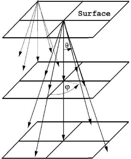
Figure 2.: The Feautrier equation is solved along one vertical and 4 inclined rays through each point on the surface. Values of the opacity and source function are interpolated to the intersection of the ray with each horizontal plane. The azimuthal angle $\phi$ of the inclined rays is rotated 15 degrees each time step in order to sample the surrounding medium.

Each $\Theta,\phi$ combination is treated in turn. For each, there is a collection of parallel rays labeled by the surface grid point through which they pass. For the slanted rays, the opacity and source function are interpolated to the location of the intersections of the rays with each horizontal plane. The optical depth along each ray at each horizontal plane is then calculated by integrating along the ray from the surface inward. Since the opacity groups are fixed multiples (10) of each other, the optical depth needs to be calculated for the continuum only and is then scaled for the other opacity groups.

To obtain accurate integrated intensities the continuum opacity average is renormalized slightly, with a factor (close to unity) obtained by requiring that the emergent intensity, summed over the four bins, should match the wavelength integrated monochromatic intensity, computed in a two-dimensional strip from the model. A posteriori checks, where similar comparisons are made for 3-D snapshots, have been used to verify the procedure.

It is crucial that the thin surface thermal boundary layer be resolved in order for the correct radiative losses to be obtained. Therefore, in low resolution simulations we interpolate from the hydrodynamic computational grid to a finer grid in the vertical direction for solving the radiation transport. In high resolution simulations this is not necessary because the thermal boundary layer is already resolved on the dynamic grid.

At large optical depths, $P_{\lambda}\rightarrow B_{\lambda}$, which leads to roundoff errors in the heating $q_{\lambda}=P_{\lambda}-B_{\lambda}$. We therefore solve the Feautrier equation directly for $q_{\lambda}=P_{\lambda}-B_{\lambda}$, by rewriting it as

$${{d^{2}q_{\lambda}}\over{d\tau_{\lambda}^{2}}}=q_{\lambda}-{{d^{2}B_{\lambda}}\over{d\tau_{\lambda}^{2}}}\ .$$ (5)

This ensures that the radiative heating/cooling goes to the correct asymptotic solution at large optical depth. The boundary conditions are

$${{dq_{\lambda}}\over{d\tau_{\lambda}}} = q_{\lambda}+B_{\lambda}-{{dB_{\lambda}}\over{d\tau_{\lambda}}}\qquad(\tau\rightarrow 0)$$

$$q_{\lambda} \rightarrow 0, \qquad(\tau\rightarrow\infty)$$

The finite difference form of the Feautrier equation is,

$$q_{j-1}\left({{1}\over{\tau_{j}-\tau_{j-1}}}\right.\left.{{2}\over{\tau_{j+1}-\tau_{j-1}}}\right)-q_{j}\left[1+\left({{1}\over{\tau_{j}-\tau_{j-1}}}+{{1}\over{\tau_{j+1}-\tau_{j}}}\right){{2}\over{\tau_{j+1}-\tau_{j-1}}}\right]$$

$$+q_{j+1}\left({{1}\over{\tau_{j+1}-\tau_{j}}}{{2}\over{\tau_{j+1}-\tau_{j-1}}}\right)=$$

$$S_{j-1}\left({{1}\over{\tau_{j}-\tau_{j-1}}}\right.\left.{{2}\over{\tau_{j+1}-\tau_{j-1}}}\right)-S_{j}\left[\left({{1}\over{\tau_{j}-\tau_{j-1}}}+{{1}\over{\tau_{j+1}-\tau_{j}}}\right){{2}\over{\tau_{j+1}-\tau_{j-1}}}\right]$$

$$S_{j+1}\left({{1}\over{\tau_{j+1}-\tau_{j}}}\right.\left.{{2}\over{\tau_{j+1}-\tau_{j-1}}}\right)\ .$$

This has the tri-diagonal form

$$A_{j}q_{j-1}+B_{j}q_{j}+C_{j}q_{j+1}=D_{j}\ .$$

There is a roundoff error problem at small optical depth, because the $1$ in $B_{j}$ becomes so small compared to $1/\Delta\tau^{2}$ that it is lost in the noise and the solution becomes indeterminate. As a result, this formulation can only be used down to optical depths the order of the square root of the machine word length. The solution is to store the sum of the tridiagonal matrix elements, rather than $B_{j}$, in the diagonal slot (Nordlund 1982, Rybicki & Hummer 1991), initializing it with

$$D_{j}==A_{j}+B_{j}+C_{j}=-1$$

The tridiagonal system is solved by the standard elimination procedure, except that the diagonal element $B_{j}$ is recovered just before the back-substitution step, where it may be obtained from

$$B_{j}=D_{j}-C_{j}\ ,$$

since at that point $A_{j}=0$ from the forward elimination.

With these substitutions, the solution is accurate for arbitrarily small optical depths.

Total radiative heating/cooling at each location where a ray crosses a horizontal coordinate surface is accumulated as the sum over opacity bins ($i=1,4$), and angles of the Feautrier $q_{i}(\theta,\phi)$,

$$Q_{\rm rad}=4\pi\sum_{\Omega}\sum_{i}\kappa_{i}q_{i}(\Omega)w_{i}w_{\Omega}\ .$$ (6)

The radiative heating/cooling is finally interpolated from the slanted grid back to the Cartesian computational grid and added into the expression for the time derivative of the internal energy and the variables are advanced in time.

5. Interaction of Radiation and Convection

The interaction between radiative and convective energy transport has a profound effect on the structure, dynamics and diagnostics of the Sun. Escaping radiation cools the plasma that reaches the solar surface and produces the low entropy plasma whose buoyancy work drives the convection. Radiative, convective and wave energy transport determines the mean structure of the solar atmosphere. Radiation emerging from the atmosphere provides the diagnostics that we use to determine the velocity, density, temperature and magnetic field on the Sun. Radiation transport modifies the observable p-mode temperature fluctuations so as to reverse the asymmetry of the intensity vs. velocity spectral peaks.

5.1. Convection Driver

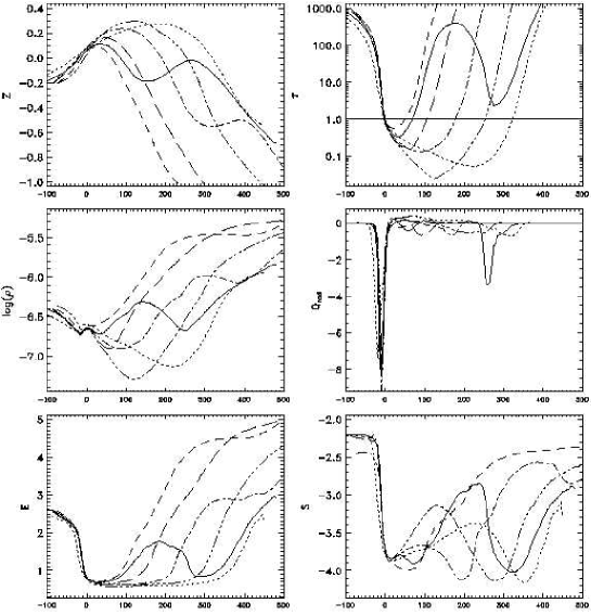
Figure 3.: Fluid that approaches the surface is cooled by radiating away its thermal and ionization energy. This decrease its entropy and it is pulled down by gravity to form the cores of downflow plumes. The largest entropy fluctuations and most of the buoyancy work that drives the convection occurs in the downflows.

Solar convection is driven primarily from a thin surface thermal boundary layer by radiative cooling. Fluid that approaches the surface loses its thermal and ionization energy to escaping radiation (Fig 3). This reduces its entropy, so gravity pulls it down to form the cores of the downflows. Large entropy fluctuations occur only in these downflows, so that most of the buoyancy work that drives the convection occurs in these downflows. Thus the primary driver of solar convection is radiative cooling from the surface (Stein & Nordlund 1998).

5.2. Atmospheric Structure

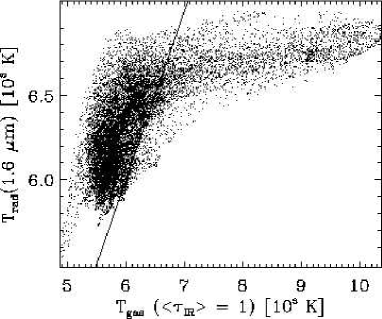
Figure 4.: Radiation temperature in the IR at 1.6 ${\mu}$m vs. gas temperature at $<\tau_{IR}>=1$. Hot gas is not observed. The large temperature sensitivity of the H^- opacity leads to large optical depths where the gas is hot and hides it from view. Thus the average gas temperature is higher than the observed radiation temperature, so the 3D atmosphere is more extended than a 1D atmosphere with the same effective temperature.

The average structure of the solar atmosphere is significantly different from that of 1D models that reproduce the observed solar luminosity and radius. First, due to 3D radiative transfer effects the average temperature of a 3D model is higher than a 1D model with the same effective temperature. The great temperature sensitivity of the H^- opacity makes the optical depth of hot gas very large, so it is not observed (Fig 4). Hence, the actual average gas temperature is higher than the observed radiation temperature. A hotter atmosphere has a larger pressure scale height and is more extended. In the solar case this gives an extra 75 km extension to the atmosphere. Second, turbulent pressure gives extra support to the atmosphere, which extends it an additional 75 km. (Fig 5) (Rosenthal et al. 1999).

Figure 5.: Atmospheric stratification is extended $\sim$ 150 km, half by 3D radiative transfer effects (Fig 4) and half by turbulent pressure support.

5.3. Atmospheric Diagnostics

 

Figure 6.: Granulation size spectrum and emergent intensity distribution compared to observed values.

Emerging continuum and line radiation provides us with the diagnostic tools to determine the properties of the solar atmosphere. Emergent radiation from the solar surface can be resolved spatially and temporally. In the continuum radiation we see the granulation. The spatial spectrum (Fig 6) gives the power in the different scales of motion. The intensity distribution tells us about the temperature contrast on the unit optical depth surface.

  

Figure 7.: Average line profile for Fe $\lambda$ 541.4 line, with temperature structure from the simulation, with no velocities (left) and with the full velocity field (right).

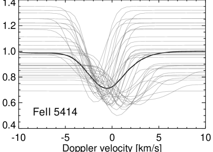
Figure 8.: The average line profile (heavy line and Fig 7) is the combination of profiles from different locations with different line shifts and widths. The effects that are modeled by micro- and macro- turbulence in 1D are all due to the overshooting convection velocities.

Line radiation gives us much more information. Spectral lines of heavy elements, whose thermal Doppler widths are small compared to typical photospheric velocities, provide direct diagnostics of velocity and temperature fluctuations in the photosphere. Non-spatially resolved properties such as average line profiles are useful because they bypass the difficulties associated with atmospheric seeing and instrumental resolution. Their shape critically depends on the solar velocity field – the temperature structure alone gives lines that are too narrow and deep (Fig 7 (left)). Including the convective overshoot velocities in the photosphere gives excellent agreement with the observed profiles (Fig 7 (right)). This observed average profile is the result of spatial and temporal averaging of lines from different locations with different temperatures and line of sight velocities and very different shifts, widths and shapes (Fig 8). The average line profile results entirely from convection induced temperature and velocity fluctuations, without any need for micro- or macro- turbulence or extra damping (Stein & Nordlund 2000).

 

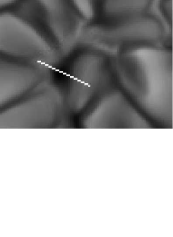
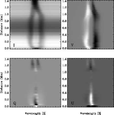
Figure 9.: Stokes profiles of FeI 630.1 nm (right) along a slit across a micropore, whose intensity image is shown on the left.

The surface magnetic field can also be determined by analyzing stokes component line profiles. An example of the stokes profiles along a slit across a micropore in the simulation is shown in Fig. 9.

5.4. P-Modes

The solar p-modes are excited by the work of turbulent pressure and non-adiabatic gas pressure (entropy) fluctuations near the top of the convection zone (Fig 10). The turbulent pressure is due to the convective motions. The entropy fluctuations result from the instantaneous local imbalance between the convective heating and radiative cooling. P-mode excitation decreases at low frequencies because of the increasing mode mass and decreasing mode compression as the frequency decreases. Excitation decreases at high frequencies because the pressure fluctuations produced by the convection fall off with increasing frequency. The modes are excited fairly close to the solar surface – the higher the frequency the closer to the surface is their excitation (Fig 10) (Stein & Nordlund 2001).

 

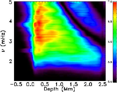
Figure 10.: Solar p-modes are excited by the work of turbulent pressure and non-adiabatic gas pressure fluctuations. The excitation is confined closer to the surface as the frequency increases.

The velocity and intensity spectra of the p-modes have asymmetric peaks. The velocity has more power on the low frequency side of the peak and the intensity has more power on the high frequency side of the peak. The velocity and intensity measured at a fixed geometrical depth have the same asymmetry, which depends on the locations of the excitation source and the observations (Kumar & Basu 1999, Georgobiani et al. 2000). The intensity asymmetry gets reversed from that of the temperature by radiation effects. The dominant H^- opacity is very temperature sensitive. The oscillation induced temperature fluctuations are larger on the low frequency side of the resonance and produce opacity changes that vary the location of radiation emission ($\tau=1)$ in a way that reduces the magnitude of the temperature fluctuations more on the low frequency side of the resonance, and thus reverses the asymmetry of the observed temperature fluctuations (Figs 11, 12).

 

Figure 11.: Velocity (solid) and temperature (dotted) spectra at fixed geometrical depth $<\tau>=1$ (left) and optical depth $\tau=1$ (right), for the first non-radial fundamental mode (corresponding to solar mode with $\ell=740$). Radiation transfer reduces the observed temperature fluctuations by over an order of magnitude and reverses the asymmetry of the temperature profile.

 

Figure 12.: Opacity (left) and height of optical depth unity (right). Larger temperature fluctuations (dotted) at frequencies below the mode peak generate larger opacity fluctuations, which in turn produce larger fluctuations in the height of the $\tau=1$ surface. This decreases the temperature fluctuations more below the peak than above it and reverses the asymmetry of the intensity with respect to the velocity.

6. Discussion

In order to make realistic numerical simulations it is necessary to include the relevant realistic physics. In the case of the solar atmosphere this means including an appropriately realistic treatment of the radiative losses. Many techniques are available to solve for radiation transport. The problem is to devise a method that is efficient enough to be applied at each time step in a dynamic calculation.

We have described a method developed by Nordlund that relies on reducing the number of frequencies that need to be treated to a bare minimum of 4, by using a multi-group binning of the wavelengths according to their opacity. In addition a minimal number of rays are employed, but they are rotated to cover the computational domain. Because we are only interested in the photosphere, we also can assume LTE. Some of the approximations we use, such as assuming that all the opacities have the same depth dependence, can be easily improved. It was instituted in a time when computer memory was small and the table size needed to be minimized. It would be nice to replace the approximation of multi-group opacities with an opacity sampling method, so as to include the effect of Doppler shifts on the radiation absorption, but the cost will be many more frequencies that need to be solved. For the Sun we are lucky that the radiation heating/cooling time scale is of the same order as the dynamical time scale, so that an explicit solution of the radiation transport is possible. For giant stars, for instance, where the dynamical time scale is much longer than the Sun’s, explicit solution of the radiation transport will reduce the possible time step size.

For other investigations, other physics will be needed. To include the chromosphere it is necessary to include at least the dominant non-LTE effects of scattering and hydrogen ionization. This is the next project we are working on in collaboration with Mats Carlsson, Viggo Hansteen and Andrew McMurray of Oslo University.

Acknowledgments.

The work of RFS was supported in part by NASA grant NAG 5 9563, NSF grants AST 9819799 and ATM 9988111. ÅN was supported in part by the Danish Research Foundation, through its establishment of the Theoretical Astrophysics Center. The calculations were performed at the National Center for Supercomputer Applications, which is supported by the National Science Foundation, at Michigan State University and at UNI$\bullet$C, Denmark. This valuable support is greatly appreciated.

References

Georgobiani, D. G., Kosovichev, A. G., Nigam, R., Nordlund, Å., & Stein, R. F. 2000, ApJ, 530, L139

Gustafsson, B., Bell, R. Eriksson, K. & Nordlund, Å. 1975, A&A, 42, 407

Kumar, P. & Basu, S. 1999, ApJ, 519, 389

Magain, P. 1983, A&A, 122, 225

Nordlund, Å, 1982, A&A, 107, 1

Rosenthal, C. S., Christensen-Dalsgaard, J., Nordlund, Å., Stein, R. F., & Trampedach, R. 1999, A&A, 351, 689

Rybicki, G. B. & Hummer, D. G. 1991, A&A, 245, 171

Skartlien, R. 2000, ApJ, 536, 465

Stein, R. F. & Nordlund, Å. 1998, ApJ, 499, 914

Stein, R. F. & Nordlund, Å. 2000, Sol. Phys., 192, 91

Stein, R. F. & Nordlund, Å. 2001, ApJ, 546, 585